#python ones and zeros array

[tparadox]

While I was able to use the holiday Monday at work to catch up on stuff I haven't been able to do in the last six weeks I've been doing my job alone, I spent way more of that time than I wanted to in trying to find a way around Excel breaking my labor saving spreadsheet by refusing to follow its own rules.

I help out my supervisor by turning the reports our phone system generates into a chart of call times she can analyze for coverage purposes. There are two hurdles the way it generates the reports creates. One of them is that the date, beginning time, and ending time, are all in the same cell of its line, and the other is that if there's no active call time in that span, it will more likely than not skip that span.

The easiest way I've come up with to find those times it skipped is to break up the time stamps into separate date, start, and stop cells, and then use conditional formatting to highlight the start times that are different from the end time of the line above. Originally I was using text to columns to do this, but then I decided I wanted to automate that. I set up a spreadsheet that would take the file name of the report and fetch the date and time cell from it, then an array of cells using the MID function to pull out the individual pieces of it.

It worked great! I could just tell it the file to look at and it got the data I needed. And then I'd go to add a line for a skipped time span and all of the formulas would break, because they were referenced based on the line number, and Excel ever so helpfully updates those references when your data moves. But it's okay because if you don't want the reference to be updated, there's a character for that. To keep the same line number, use B$2 instead of B2.

I worked out a fancy formula with INDIRECT, LEFT, and the new to me FORMULATEXT function to automatically assemble a new version of the formula with the crucial absolute reference for each row, since the absolute meant it wouldn't update by line if I just filled down and I was not going into over 300 cells to add one character by hand.

EXCEPT! Marking the reference as absolute only freezes the reference for pasting and directional filling! It turns out it totally ignores the $ if you're shifting and inserting! Excel broke my plans because it doesn't follow its own rules!

After like two hours of beating my head against it and reading a bunch of forum help threads where the answer was "just use INDIRECT" when I was already using INDIRECT, using COUNTIF to count only the cells above that had data in them seemed promising, but it kept giving reference errors as part of the INDIRECT, probably because the COUNTIF syntax needs you to tell it what to look for, and I think the quotation marks around the asterisk weren't playing nicely with the quotation marks of the INDIRECT even though I was using " for the latter and ' for the former. Finally I started looking into other COUNT_____ functions and it turns out that plan old COUNT does exactly what I was looking for. Where "count cells that have data" with COUNTIF needs you to specify cells containing "*", COUNT just does it. By some miracle, I found the right syntax to have the INDIRECT assemble the COUNT with a range from B1 to (current cell) in only one or two tries, and now I finally have a formula that doesn't care if I add lines which are empty in the column it's looking at.

Now I just need to automate adding the missing rows and filling in the zero values in the column I'm doing this all for, but that seems beyond what I can do with just Excel on its own. Seems like something that would be simple to execute in Python if I export a CSV, and if I could get anything to work in VBasic I could probably do a macro, but I'd prefer not to step it out of Excel and back in, and I don't think our workstations have Python, and if they don't have it, I can't add it...

[react-js-state-1]

Why Java Is Still the King in 2025—and How Cyberinfomines Makes You Job-Ready with It

1. Java in 2025: Still Relevant, Still Dominating��Despite the rise of new languages like Python, Go, and Rust, Java is far from dead—it’s actually thriving.

In 2025, Java powers:

40%+ of enterprise backend systems

90% of Android apps

Global banking & fintech infrastructures

E-commerce giants like Amazon, Flipkart & Alibaba

Microservices and cloud-native platforms using Spring Boot

Java is reliable, scalable, and highly in demand. But just learning syntax won’t get you hired. You need hands-on experience, framework expertise, and the ability to solve real-world problems.

That’s exactly what Cyberinfomines delivers.

2. The Problem: Why Most Java Learners Don’t Get Jobs Many students learn Java but still fail to land jobs. Why?

❌ They focus only on theory ❌ They memorize code, don’t build projects ❌ No real understanding of frameworks like Spring Boot ❌ Can’t explain their code in interviews ❌ Lack of problem-solving or debugging skills

That’s where Cyberinfomines’ Training changes the game—we teach Java like it’s used in real companies.

3. How Cyberinfomines Bridges the Gap At Cyberinfomines, we:

✅ Teach Core + Advanced Java with daily coding tasks ✅ Use real-world problem statements (not academic ones) ✅ Give exposure to tools like IntelliJ, Git, Maven ✅ Build full-stack projects using Spring Boot + MySQL ✅ Run mock interviews and HR prep ✅ Help you create a Java portfolio for recruiters

And yes—placement support is part of the package.

4. Java Course Curriculum: Built for the Real World Core Java

Data types, loops, arrays, OOP principles

Exception handling, packages, constructors

File handling & multithreading

Classes vs Interfaces

String manipulation & memory management

Advanced Java

JDBC (Java Database Connectivity)

Servlet Lifecycle

JSP (Java Server Pages)

HTTP Requests & Responses

MVC Design Pattern

Spring Framework + Spring Boot

Dependency Injection & Beans

Spring Data JPA

RESTful API Creation

Security & authentication

Connecting with front-end apps (React/Angular)

Tools Covered

IntelliJ IDEA

Eclipse

Postman

Git & GitHub

MySQL & Hibernate

Live Projects

Library Management System

Employee Leave Tracker

E-Commerce REST API

Blog App with full CRUD

Interview Preparation

DSA using Java

Java-based coding problems

100+ mock interview questions

HR round preparation

Resume writing workshops

5. Who Should Learn Java in 2025? You should choose Java if you are:

 A fresher who wants a strong foundation

 A non-tech graduate looking to switch to IT

 A teacher/trainer who wants to upskill

 A professional aiming for backend roles

 Someone interested in Android development

A student looking to crack placement drives or government IT jobs

6. Real Success Stories from Our Java Learners

Amit (BSc Graduate) – Now working as a Java backend developer at an IT firm in Pune. Built his confidence with live projects and mock tests.

Pooja (Mechanical Engineer) – Switched from core to IT after completing Cyberinfomines’ Java program. Cracked TCS with flying colors.

Rahul (Dropout) – Didn’t finish college but now works remotely as a freelance Spring Boot developer for a US-based startup.

Every story started with zero coding experience. They ended with real jobs.

7. Top Java Careers in 2025 & Salary Trends In-demand roles include:

Java Backend Developer

Full Stack Developer (Java + React)

Android Developer (Java)

Spring Boot Microservices Architect

QA Automation with Java + Selenium

API Developer (Spring + REST)

Starting salary: ₹4.5 – ₹8 LPA (for freshers with strong skills) Mid-level: ₹10 – ₹20 LPA Freelancers: ₹1,000 – ₹2,500/hour

Java is stable, scalable, and pays well.

8. Certifications, Tools & Practical Add-Ons After training, you’ll earn:

Cyberinfomines Java Developer Certificate

Portfolio with at least 3 GitHub-hosted projects

Proficiency in IntelliJ, Maven, Git, MySQL

Resume aligned with Java job descriptions

Interview recordings and performance feedback

9. What Makes Cyberinfomines Java Training Different

✔ Human mentorship, not just videos ✔ Doubt sessions + code reviews ✔ Classes in Hindi & English ✔ Live assignments + evaluation ✔ Placement-oriented approach ✔ No-nonsense teaching. Only what’s needed for jobs.

We focus on you becoming employable, not just completing a course.

10. Final Words: Code Your Future with Confidence Java in 2025 isn’t just relevant—it’s crucial.

And with Cyberinfomines, you don’t just learn Java.

You learn how to:

Solve real problems

Write clean, scalable code

Work like a developer

Get hired faster

Whether you’re starting fresh or switching paths, our Java course gives you the skills and confidence you need to build a future-proof career.

📞 Have questions? Want to get started?

Contact us today: 📧 vidhya.chandel@cyberinfomines.com 📞 +91-8587000904-905, 9643424141 🌐 Visit: www.cyberinfomines.com

[subb01]

Python for Data Science: The Only Guide You Need to Get Started in 2025

Data is the lifeblood of modern business, powering decisions in healthcare, finance, marketing, sports, and more. And at the core of it all lies a powerful and beginner-friendly programming language — Python.

Whether you’re an aspiring data scientist, analyst, or tech enthusiast, learning Python for data science is one of the smartest career moves you can make in 2025.

In this guide, you’ll learn:

Why Python is the preferred language for data science

The libraries and tools you must master

A beginner-friendly roadmap

How to get started with a free full course on YouTube

Why Python is the #1 Language for Data Science

Python has earned its reputation as the go-to language for data science and here's why:

1. Easy to Learn, Easy to Use

Python’s syntax is clean, simple, and intuitive. You can focus on solving problems rather than struggling with the language itself.

2. Rich Ecosystem of Libraries

Python offers thousands of specialized libraries for data analysis, machine learning, and visualization.

3. Community and Resources

With a vibrant global community, you’ll never run out of tutorials, forums, or project ideas to help you grow.

4. Integration with Tools & Platforms

From Jupyter notebooks to cloud platforms like AWS and Google Colab, Python works seamlessly everywhere.

What You Can Do with Python in Data Science

Let’s look at real tasks you can perform using Python: TaskPython ToolsData cleaning & manipulationPandas, NumPyData visualizationMatplotlib, Seaborn, PlotlyMachine learningScikit-learn, XGBoostDeep learningTensorFlow, PyTorchStatistical analysisStatsmodels, SciPyBig data integrationPySpark, Dask

Python lets you go from raw data to actionable insight — all within a single ecosystem.

A Beginner's Roadmap to Learn Python for Data Science

If you're starting from scratch, follow this step-by-step learning path:

✅ Step 1: Learn Python Basics

Variables, data types, loops, conditionals

Functions, file handling, error handling

✅ Step 2: Explore NumPy

Arrays, broadcasting, numerical computations

✅ Step 3: Master Pandas

DataFrames, filtering, grouping, merging datasets

✅ Step 4: Visualize with Matplotlib & Seaborn

Create charts, plots, and visual dashboards

✅ Step 5: Intro to Machine Learning

Use Scikit-learn for classification, regression, clustering

✅ Step 6: Work on Real Projects

Apply your knowledge to real-world datasets (Kaggle, UCI, etc.)

Who Should Learn Python for Data Science?

Python is incredibly beginner-friendly and widely used, making it ideal for:

Students looking to future-proof their careers

Working professionals planning a transition to data

Analysts who want to automate and scale insights

Researchers working with data-driven models

Developers diving into AI, ML, or automation

How Long Does It Take to Learn?

You can grasp Python fundamentals in 2–3 weeks with consistent daily practice. To become proficient in data science using Python, expect to spend 3–6 months, depending on your pace and project experience.

The good news? You don’t need to do it alone.

🎓 Learn Python for Data Science – Full Free Course on YouTube

We’ve put together a FREE, beginner-friendly YouTube course that covers everything you need to start your data science journey using Python.

📘 What You’ll Learn:

Python programming basics

NumPy and Pandas for data handling

Matplotlib for visualization

Scikit-learn for machine learning

Real-life datasets and projects

Step-by-step explanations

📺 Watch the full course now → 👉 Python for Data Science Full Course

You’ll walk away with job-ready skills and project experience — at zero cost.

🧭 Final Thoughts

Python isn’t just a programming language — it’s your gateway to the future.

By learning Python for data science, you unlock opportunities across industries, roles, and technologies. The demand is high, the tools are ready, and the learning path is clearer than ever.

Don’t let analysis paralysis hold you back.

Click here to start learning now → https://youtu.be/6rYVt_2q_BM

#PythonForDataScience #LearnPython #FreeCourse #DataScience2025 #MachineLearning #NumPy #Pandas #DataAnalysis #AI #ScikitLearn #UpskillNow

[korshubudemycoursesblog]

Unlock Your Coding Superpower: Mastering Python, Pandas, Numpy for Absolute Beginners

If you've ever thought programming looked like a superpower — something only a chosen few could wield — it's time to change that narrative. Learning to code is no longer a mystery, and Python is your easiest gateway into this world. But what if you're a complete beginner? No background, no experience, no idea where to start?

Good news: Python, Pandas, and NumPy were practically made for you.

In this blog, we’ll walk you through why these tools are ideal for anyone just starting out. And if you want a structured, guided path, we highly recommend diving into this complete beginner-friendly course: 👉 Mastering Python, Pandas, Numpy for Absolute Beginners 👈

Let’s start unlocking your coding potential — one simple step at a time.

Why Start With Python?

Let’s keep it real. Python is one of the most beginner-friendly programming languages out there. Its syntax is clear, clean, and intuitive — almost like writing English. This makes it the perfect entry point for new coders.

Here’s what makes Python shine for absolute beginners:

Easy to Read and Write: You don’t need to memorize complex symbols or deal with cryptic syntax.

Huge Community Support: Got stuck? The internet is full of answers — from Stack Overflow to YouTube tutorials.

Used Everywhere: From web development to data analysis, Python is behind some of the world’s most powerful applications.

So whether you want to analyze data, automate tasks, or build apps, Python is your go-to language.

Where Do Pandas and NumPy Fit In?

Great question.

While Python is the language, Pandas and NumPy are the power tools that make data handling and analysis easy and efficient.

🧠 What Is NumPy?

NumPy (short for Numerical Python) is a library designed for high-performance numerical computing. In simple terms, it helps you do math with arrays — fast and efficiently.

Think of NumPy like your calculator, but 10x smarter and faster. It's perfect for:

Performing mathematical operations on large datasets

Creating multi-dimensional arrays

Working with matrices and linear algebra

🧠 What Is Pandas?

If NumPy is your calculator, Pandas is your Excel on steroids.

Pandas is a Python library that lets you manipulate, analyze, and clean data in tabular form (just like spreadsheets). It’s ideal for:

Importing CSV or Excel files

Cleaning messy data

Analyzing large datasets quickly

In short: Pandas + NumPy + Python = Data Analysis Superpowers.

Real Talk: Why You Should Learn This Trio Now

The demand for Python programmers, especially those who can work with data, has skyrocketed. From tech companies to banks, from hospitals to online retailers — data is the currency, and Python is the language of that currency.

Still unsure? Let’s break down the benefits:

1. No Prior Experience Needed

This trio doesn’t assume you’ve written a single line of code. It's designed for learners who are starting from ground zero.

2. Fast Career Opportunities

Roles like Data Analyst, Python Developer, or even Automation Tester are open to beginners with these skills.

3. Used by Top Companies

Google, Netflix, NASA — they all use Python with Pandas and NumPy in various ways.

4. Perfect for Freelancers and Entrepreneurs

Want to automate your invoices, sort data, or build small tools for clients? This skillset is gold.

What You’ll Learn in the Course (and Why It Works)

The course Mastering Python, Pandas, Numpy for Absolute Beginners is not just a crash course — it’s a well-paced, thoughtfully designed bootcamp that makes learning fun, easy, and practical.

Here's what makes it a winner:

✅ Step-by-Step Python Foundation

Install Python and set up your workspace

Learn variables, loops, functions, and conditionals

Build confidence with coding exercises

✅ Hands-On NumPy Training

Create arrays and matrices

Use NumPy’s built-in functions for quick calculations

Apply real-life examples to understand concepts better

✅ Practical Pandas Projects

Import and clean data from files

Slice, filter, and aggregate data

Create powerful visualizations and summaries

✅ Real-World Applications

From data cleaning to basic automation, this course helps you build practical projects that show up on portfolios and get noticed by recruiters.

✅ Learn at Your Own Pace

No pressure. You can go slow or fast, revisit lessons, and even practice with downloadable resources.

From Absolute Beginner to Confident Coder — Your Journey Starts Here

Let’s paint a picture.

You’re sitting at your laptop, coffee in hand. You type a few lines of code. You see the output — data neatly cleaned, or graphs beautifully rendered. It clicks. You feel empowered. You’re not just learning code anymore — you’re using it.

That’s the journey this course promises. It doesn’t throw complex concepts at you. It holds your hand and builds your confidence until you feel like you can take on real-world problems.

And the best part? You’ll be surprised how quickly things start making sense.

👉 Ready to experience that feeling? Enroll in Mastering Python, Pandas, Numpy for Absolute Beginners

Common Myths (And Why They’re Wrong)

Before we wrap up, let’s bust a few myths that might be holding you back.

❌ “I need a math or computer science background.”

Nope. This course is designed for non-tech people. It’s friendly, guided, and explained in simple language.

❌ “It’ll take years to learn.”

Wrong again. You’ll be surprised how much you can learn in just a few weeks if you stay consistent.

❌ “It’s only useful for data scientists.”

Python, Pandas, and NumPy are used in marketing, HR, finance, healthcare, e-commerce — the list goes on.

What Past Learners Are Saying

“I was terrified to even open Python. Now I’m analyzing datasets like a pro. This course literally changed my life!” – Priya K., Student

“I tried learning on YouTube but kept getting confused. This course explained things step-by-step. I finally get it.” – James M., Freelancer

“As a small business owner, I used Python to automate my reports. Saved me hours every week.” – Aamir T., Entrepreneur

Your First Step Starts Today

You don’t need to be a genius to learn Python. You just need a guide, a plan, and a little bit of curiosity.

Python, Pandas, and NumPy are your starting tools — powerful enough to transform how you work, think, and problem-solve. And once you begin, you'll wonder why you didn’t start sooner.

So why wait?

🚀 Click here to start your learning journey today: 👉 Mastering Python, Pandas, Numpy for Absolute Beginners

[codingbrushup]

Top 10 Free Coding Tutorials on Coding Brushup You Shouldn’t Miss

If you're passionate about learning to code or just starting your programming journey, Coding Brushup is your go-to platform. With a wide range of beginner-friendly and intermediate tutorials, it’s built to help you brush up your skills in languages like Java, Python, and web development technologies. Best of all? Many of the tutorials are absolutely free.

In this blog, we’ll highlight the top 10 free coding tutorials on Coding BrushUp that you simply shouldn’t miss. Whether you're aiming to master the basics or explore real-world projects, these tutorials will give you the knowledge boost you need.

1. Introduction to Python Programming – Coding BrushUp Python Tutorial

Python is one of the most beginner-friendly languages, and the Coding BrushUp Python Tutorial series starts you off with the fundamentals. This course covers:

●     Setting up Python on your machine

●     Variables, data types, and basic syntax

●     Loops, functions, and conditionals

●     A mini project to apply your skills

Whether you're a student or an aspiring data analyst, this free tutorial is perfect for building a strong foundation.

📌 Try it here: Coding BrushUp Python Tutorial

2. Java for Absolute Beginners – Coding BrushUp Java Tutorial

Java is widely used in Android development and enterprise software. The Coding BrushUp Java Tutorial is designed for complete beginners, offering a step-by-step guide that includes:

●     Setting up Java and IntelliJ IDEA or Eclipse

●     Understanding object-oriented programming (OOP)

●     Working with classes, objects, and inheritance

●     Creating a simple console-based application

This tutorial is one of the highest-rated courses on the site and is a great entry point into serious backend development.

📌 Explore it here: Coding BrushUp Java Tutorial

3. Build a Personal Portfolio Website with HTML & CSS

Learning to create your own website is an essential skill. This hands-on tutorial walks you through building a personal portfolio using just HTML and CSS. You'll learn:

●     Basic structure of HTML5

●     Styling with modern CSS3

●     Responsive layout techniques

●     Hosting your portfolio online

Perfect for freelancers and job seekers looking to showcase their skills.

4. JavaScript Basics: From Zero to DOM Manipulation

JavaScript powers the interactivity on the web, and this tutorial gives you a solid introduction. Key topics include:

●     JavaScript syntax and variables

●     Functions and events

●     DOM selection and manipulation

●     Simple dynamic web page project

By the end, you'll know how to create interactive web elements without relying on frameworks.

5. Version Control with Git and GitHub – Beginner’s Guide

Knowing how to use Git is essential for collaboration and managing code changes. This free tutorial covers:

●     Installing Git

●     Basic Git commands: clone, commit, push, pull

●     Branching and merging

●     Using GitHub to host and share your code

Even if you're a solo developer, mastering Git early will save you time and headaches later.

6. Simple CRUD App with Java (Console-Based)

In this tutorial, Coding BrushUp teaches you how to create a simple CRUD (Create, Read, Update, Delete) application in Java. It's a great continuation after the Coding Brushup Java Course Tutorial. You'll learn:

●     Working with Java arrays or Array List

●     Creating menu-driven applications

●     Handling user input with Scanner

●     Structuring reusable methods

This project-based learning reinforces core programming concepts and logic building.

7. Python for Data Analysis: A Crash Course

If you're interested in data science or analytics, this Coding Brushup Python Tutorial focuses on:

●     Using libraries like Pandas and NumPy

●     Reading and analyzing CSV files

●     Data visualization with Matplotlib

●     Performing basic statistical operations

It’s a fast-track intro to one of the hottest career paths in tech.

8. Responsive Web Design with Flexbox and Grid

This tutorial dives into two powerful layout modules in CSS:

●     Flexbox: for one-dimensional layouts

●     Grid: for two-dimensional layouts

You’ll build multiple responsive sections and gain experience with media queries, making your websites look great on all screen sizes.

9. Java Object-Oriented Concepts – Intermediate Java Tutorial

For those who’ve already completed the Coding Brushup Java Tutorial, this intermediate course is the next logical step. It explores:

●     Inheritance and polymorphism

●     Interfaces and abstract classes

●     Encapsulation and access modifiers

●     Real-world Java class design examples

You’ll write cleaner, modular code and get comfortable with real-world Java applications.

10. Build a Mini Calculator with Python (GUI Version)

This hands-on Coding BrushUp Python Tutorial teaches you how to build a desktop calculator using Tkinter, a built-in Python GUI library. You’ll learn:

●     GUI design principles

●     Button, entry, and event handling

●     Function mapping and error checking

●     Packaging a desktop application

A fun and visual way to practice Python programming!

Why Choose Coding BrushUp?

Coding BrushUp is more than just a collection of tutorials. Here’s what sets it apart:

✅ Clear Explanations – All lessons are written in plain English, ideal for beginners.  ✅ Hands-On Projects – Practical coding exercises to reinforce learning.  ✅ Progressive Learning Paths – Start from basics and grow into advanced topics.  ✅ 100% Free Content – Many tutorials require no signup or payment.  ✅ Community Support – Comment sections and occasional Q&A features allow learner interaction.

Final Thoughts

Whether you’re learning to code for career advancement, school, or personal development, the free tutorials at Coding Brushup offer valuable, structured, and practical knowledge. From mastering the basics of Python and Java to building your first website or desktop app, these resources will help you move from beginner to confident coder.

👉 Start learning today at Codingbrushup.com and check out the full Coding BrushUp Java Tutorial and Python series to supercharge your programming journey.

[yasirinsights]

Mastering NumPy in Python – The Ultimate Guide for Data Enthusiasts

Imagine calculating the average of a million numbers using regular Python lists. You’d need to write multiple lines of code, deal with loops, and wait longer for the results. Now, what if you could do that in just one line? Enter NumPy in Python, the superhero of numerical computing in Python.

NumPy in Python (short for Numerical Python) is the core package that gives Python its scientific computing superpowers. It’s built for speed and efficiency, especially when working with arrays and matrices of numeric data. At its heart lies the ndarray—a powerful n-dimensional array object that’s much faster and more efficient than traditional Python lists.

What is NumPy in Python and Why It Matters

Why is NumPy a game-changer?

It allows operations on entire arrays without writing for-loops.

It’s written in C under the hood, so it’s lightning-fast.

It offers functionalities like Fourier transforms, linear algebra, random number generation, and so much more.

It’s compatible with nearly every scientific and data analysis library in Python like SciPy, Pandas, TensorFlow, and Matplotlib.

In short, if you’re doing data analysis, machine learning, or scientific research in Python, NumPy is your starting point.

The Evolution and Importance of NumPy in Python Ecosystem

Before NumPy in Python, Python had numeric libraries, but none were as comprehensive or fast. NumPy was developed to unify them all under one robust, extensible, and fast umbrella.

Created by Travis Oliphant in 2005, NumPy grew from an older package called Numeric. It soon became the de facto standard for numerical operations. Today, it’s the bedrock of almost every other data library in Python.

What makes it crucial?

Consistency: Most libraries convert input data into NumPy arrays for consistency.

Community: It has a huge support community, so bugs are resolved quickly and the documentation is rich.

Cross-platform: It runs on Windows, macOS, and Linux with zero change in syntax.

This tight integration across the Python data stack means that even if you’re working in Pandas or TensorFlow, you’re indirectly using NumPy under the hood.

Setting Up NumPy in Python

How to Install NumPy

Before using NumPy, you need to install it. The process is straightforward:

bash

pip install numpy

Alternatively, if you’re using a scientific Python distribution like Anaconda, NumPy comes pre-installed. You can update it using:

bash

conda update numpy

That’s it—just a few seconds, and you’re ready to start number-crunching!

Some environments (like Jupyter notebooks or Google Colab) already have NumPy installed, so you might not need to install it again.

Importing NumPy in Python and Checking Version

Once installed, you can import NumPy using the conventional alias:

python

import numpy as np

This alias, np, is universally recognized in the Python community. It keeps your code clean and concise.

To check your NumPy version:

python

print(np.__version__)

You’ll want to ensure that you’re using the latest version to access new functions, optimizations, and bug fixes.

If you’re just getting started, make it a habit to always import NumPy with np. It’s a small convention, but it speaks volumes about your code readability.

Understanding NumPy in Python Arrays

The ndarray Object – Core of NumPy

At the center of everything in NumPy lies the ndarray. This is a multidimensional, fixed-size container for elements of the same type.

Key characteristics:

Homogeneous Data: All elements are of the same data type (e.g., all integers or all floats).

Fast Operations: Built-in operations are vectorized and run at near-C speed.

Memory Efficiency: Arrays take up less space than lists.

You can create a simple array like this:

python

import numpy as np arr = np.array([1, 2, 3, 4])

Now arr is a NumPy array (ndarray), not just a Python list. The difference becomes clearer with larger data or when applying operations:

python

arr * 2 # [2 4 6 8]

It’s that easy. No loops. No complications.

You can think of an ndarray like an Excel sheet with superpowers—except it can be 1d, 2d, 3d, or even higher dimensions!

1-Dimensional Arrays – Basics and Use Cases

1d arrays are the simplest form—just a list of numbers. But don’t let the simplicity fool you. They’re incredibly powerful.

Creating a 1D array:

python

a = np.array([10, 20, 30, 40])

You can:

Multiply or divide each element by a number.

Add another array of the same size.

Apply mathematical functions like sine, logarithm, etc.

Example:

python

b = np.array([1, 2, 3, 4]) print(a + b) # Output: [11 22 33 44]

This concise syntax is possible because NumPy performs element-wise operations—automatically!

1d arrays are perfect for:

Mathematical modeling

Simple signal processing

Handling feature vectors in ML

Their real power emerges when used in batch operations. Whether you’re summing elements, calculating means, or applying a function to every value, 1D arrays keep your code clean and blazing-fast.

2-Dimensional Arrays – Matrices and Their Applications

2D arrays are like grids—rows and columns of data. They’re also the foundation of matrix operations in NumPy in Python.

You can create a 2D array like this:

python

arr_2d = np.array([[1, 2, 3], [4, 5, 6]])

Here’s what it looks like:

lua

[[1 2 3] [4 5 6]]

Each inner list becomes a row. This structure is ideal for:

Representing tables or datasets

Performing matrix operations like dot products

Image processing (since images are just 2D arrays of pixels)

Some key operations:

python

arr_2d.shape # (2, 3) — 2 rows, 3 columns arr_2d[0][1] # 2 — first row, second column arr_2d.T # Transpose: swaps rows and columns

You can also use slicing just like with 1d arrays:

python

arr_2d[:, 1] # All rows, second column => [2, 5] arr_2d[1, :] # Second row => [4, 5, 6]

2D arrays are extremely useful in:

Data science (e.g., CSVS loaded into 2D arrays)

Linear algebra (matrices)

Financial modelling and more

They’re like a spreadsheet on steroids—flexible, fast, and powerful.

3-Dimensional Arrays – Multi-Axis Data Representation

Now let’s add another layer. 3d arrays are like stacks of 2D arrays. You can think of them as arrays of matrices.

Here’s how you define one:

python

arr_3d = np.array([ [[1, 2], [3, 4]], [[5, 6], [7, 8]] ])

This array has:

2 matrices

Each matrix has 2 rows and 2 columns

Visualized as:

lua

[ [[1, 2], [3, 4]],[[5, 6], [7, 8]] ]

Accessing data:

python

arr_3d[0, 1, 1] # Output: 4 — first matrix, second row, second column

Use cases for 3D arrays:

Image processing (RGB images: height × width × color channels)

Time series data (time steps × variables × features)

Neural networks (3D tensors as input to models)

Just like with 2D arrays, NumPy’s indexing and slicing methods make it easy to manipulate and extract data from 3D arrays.

And the best part? You can still apply mathematical operations and functions just like you would with 1D or 2D arrays. It’s all uniform and intuitive.

Higher Dimensional Arrays – Going Beyond 3D

Why stop at 3D? NumPy in Python supports N-dimensional arrays (also called tensors). These are perfect when dealing with highly structured datasets, especially in advanced applications like:

Deep learning (4D/5D tensors for batching)

Scientific simulations

Medical imaging (like 3D scans over time)

Creating a 4D array:

python

arr_4d = np.random.rand(2, 3, 4, 5)

This gives you:

2 batches

Each with 3 matrices

Each matrix has 4 rows and 5 columns

That’s a lot of data—but NumPy handles it effortlessly. You can:

Access any level with intuitive slicing

Apply functions across axes

Reshape as needed using .reshape()

Use arr.ndim to check how many dimensions you’re dealing with. Combine that with .shape, and you’ll always know your array’s layout.

Higher-dimensional arrays might seem intimidating, but NumPy in Python makes them manageable. Once you get used to 2D and 3D, scaling up becomes natural.

NumPy in Python Array Creation Techniques

Creating Arrays Using Python Lists

The simplest way to make a NumPy array is by converting a regular Python list:

python

a = np.array([1, 2, 3])

Or a list of lists for 2D arrays:

python

b = np.array([[1, 2], [3, 4]])

You can also specify the data type explicitly:

python

np.array([1, 2, 3], dtype=float)

This gives you a float array [1.0, 2.0, 3.0]. You can even convert mixed-type lists, but NumPy will automatically cast to the most general type to avoid data loss.

Pro Tip: Always use lists of equal lengths when creating 2D+ arrays. Otherwise, NumPy will make a 1D array of “objects,” which ruins performance and vectorization.

Array Creation with Built-in Functions (arange, linspace, zeros, ones, etc.)

NumPy comes with handy functions to quickly create arrays without writing out all the elements.

Here are the most useful ones:

np.arange(start, stop, step): Like range() but returns an array.

np.linspace(start, stop, num): Evenly spaced numbers between two values.

np.zeros(shape): Array filled with zeros.

np.ones(shape): Array filled with ones.

np.eye(N): Identity matrix.

These functions help you prototype, test, and create arrays faster. They also avoid manual errors and ensure your arrays are initialized correctly.

Random Array Generation with random Module

Need to simulate data? NumPy’s random module is your best friend.

python

np.random.rand(2, 3) # Uniform distribution np.random.randn(2, 3) # Normal distribution np.random.randint(0, 10, (2, 3)) # Random integers

You can also:

Shuffle arrays

Choose random elements

Set seeds for reproducibility (np.random.seed(42))

This is especially useful in:

Machine learning (generating datasets)

Monte Carlo simulations

Statistical experiments.

Reshaping, Flattening, and Transposing Arrays

Reshaping is one of NumPy’s most powerful features. It lets you reorganize the shape of an array without changing its data. This is critical when preparing data for machine learning models or mathematical operations.

Here’s how to reshape:

python

a = np.array([1, 2, 3, 4, 5, 6]) b = a.reshape(2, 3) # Now it's 2 rows and 3 columns

Reshaped arrays can be converted back using .flatten():

python

flat = b.flatten() # [1 2 3 4 5 6]

There’s also .ravel()—similar to .flatten() but returns a view if possible (faster and more memory-efficient).

Transposing is another vital transformation:

python

matrix = np.array([[1, 2], [3, 4]]) matrix.T # Output: # [[1 3] # [2 4]]

Transpose is especially useful in linear algebra, machine learning (swapping features with samples), and when matching shapes for operations like matrix multiplication.

Use .reshape(-1, 1) to convert arrays into columns, and .reshape(1, -1) to make them rows. This flexibility gives you total control over the structure of your data.

Array Slicing and Indexing Tricks

You can access parts of an array using slicing, which works similarly to Python lists but more powerful in NumPy in Python.

Basic slicing:

python

arr = np.array([10, 20, 30, 40, 50]) arr[1:4] # [20 30 40]

2D slicing:

python

mat = np.array([[1, 2, 3], [4, 5, 6], [7, 8, 9]]) mat[0:2, 1:] # Rows 0-1, columns 1-2 => [[2 3], [5 6]]

Advanced indexing includes:

Boolean indexing:

python

arr[arr > 30] # Elements greater than 30

Fancy indexing:

python

arr[[0, 2, 4]] # Elements at indices 0, 2, 4

Modifying values using slices:

python

arr[1:4] = 99 # Replace elements at indices 1 to 3

Slices return views, not copies. So if you modify a slice, the original array is affected—unless you use .copy().

These slicing tricks make data wrangling fast and efficient, letting you filter and extract patterns in seconds.

Broadcasting and Vectorized Operations

Broadcasting is what makes NumPy in Python shine. It allows operations on arrays of different shapes and sizes without writing explicit loops.

Let’s say you have a 1D array:

python

a = np.array([1, 2, 3])

And a scalar:

python

b = 10

You can just write:

python

c = a + b # [11, 12, 13]

That’s broadcasting in action. It also works for arrays with mismatched shapes as long as they are compatible:

python

a = np.array([[1], [2], [3]]) # Shape (3,1) b = np.array([4, 5, 6]) # Shape (3,)a + b

This adds each element to each element b, creating a full matrix.

Why is this useful?

It avoids for-loops, making your code cleaner and faster

It matches standard mathematical notation

It enables writing expressive one-liners

Vectorization uses broadcasting behind the scenes to perform operations efficiently:

python

a * b # Element-wise multiplication np.sqrt(a) # Square root of each element np.exp(a) # Exponential of each element

These tricks make NumPy in Python code shorter, faster, and far more readable.

Mathematical and Statistical Operations

NumPy offers a rich suite of math functions out of the box.

Basic math:

python

np.add(a, b) np.subtract(a, b) np.multiply(a, b) np.divide(a, b)

Aggregate functions:

python

np.sum(a) np.mean(a) np.std(a) np.var(a) np.min(a) np.max(a)

Axis-based operations:

python

arr_2d = np.array([[1, 2, 3], [4, 5, 6]]) np.sum(arr_2d, axis=0) # Sum columns: [5 7 9] np.sum(arr_2d, axis=1) # Sum rows: [6 15]

Linear algebra operations:

python

np.dot(a, b) # Dot product np.linalg.inv(mat) # Matrix inverse np.linalg.det(mat) # Determinant np.linalg.eig(mat) # Eigenvalues

Statistical functions:

python

np.percentile(a, 75) np.median(a) np.corrcoef(a, b)

Trigonometric operations:

python

np.sin(a) np.cos(a) np.tan(a)

These functions let you crunch numbers, analyze trends, and model complex systems in just a few lines.

NumPy in Python  I/O – Saving and Loading Arrays

Data persistence is key. NumPy in Python lets you save and load arrays easily.

Saving arrays:

python

np.save('my_array.npy', a) # Saves in binary format

Loading arrays:

python

b = np.load('my_array.npy')

Saving multiple arrays:

python

np.savez('data.npz', a=a, b=b)

Loading multiple arrays:

python

data = np.load('data.npz') print(data['a']) # Access saved 'a' array

Text file operations:

python

np.savetxt('data.txt', a, delimiter=',') b = np.loadtxt('data.txt', delimiter=',')

Tips:

Use .npy or .npz formats for efficiency

Use .txt or .csv for interoperability

Always check array shapes after loading

These functions allow seamless transition between computations and storage, critical for real-world data workflows.

Masking, Filtering, and Boolean Indexing

NumPy in Python allows you to manipulate arrays with masks—a powerful way to filter and operate on elements that meet certain conditions.

Here’s how masking works:

python

arr = np.array([10, 20, 30, 40, 50]) mask = arr > 25

Now mask is a Boolean array:

graphql

[False False True True True]

You can use this mask to extract elements:

python

filtered = arr[mask] # [30 40 50]

Or do operations:

python

arr[mask] = 0 # Set all elements >25 to 0

Boolean indexing lets you do conditional replacements:

python

arr[arr < 20] = -1 # Replace all values <20

This technique is extremely useful in:

Cleaning data

Extracting subsets

Performing conditional math

It’s like SQL WHERE clauses but for arrays—and lightning-fast.

Sorting, Searching, and Counting Elements

Sorting arrays is straightforward:

python

arr = np.array([10, 5, 8, 2]) np.sort(arr) # [2 5 8 10]

If you want to know the index order:

python

np.argsort(arr) # [3 1 2 0]

Finding values:

python

np.where(arr > 5) # Indices of elements >5

Counting elements:

python

np.count_nonzero(arr > 5) # How many elements >5

You can also use np.unique() to find unique values and their counts:

python

np.unique(arr, return_counts=True)

Need to check if any or all elements meet a condition?

python

np.any(arr > 5) # True if any >5 np.all(arr > 5) # True if all >5

These operations are essential when analyzing and transforming datasets.

Copy vs View in NumPy in Python – Avoiding Pitfalls

Understanding the difference between a copy and a view can save you hours of debugging.

By default, NumPy tries to return views to save memory. But modifying a view also changes the original array.

Example of a view:

python

a = np.array([1, 2, 3]) b = a[1:] b[0] = 99 print(a) # [1 99 3] — original changed!

If you want a separate copy:

python

b = a[1:].copy()

Now b is independent.

How to check if two arrays share memory?

python

np.may_share_memory(a, b)

When working with large datasets, always ask yourself—is this a view or a copy? Misunderstanding this can lead to subtle bugs.

Useful NumPy Tips and Tricks

Let’s round up with some power-user tips:

Memory efficiency: Use dtype to optimize storage. For example, use np.int8 instead of the default int64 for small integers.

Chaining: Avoid chaining operations that create temporary arrays. Instead, use in-place ops like arr += 1.

Use .astype() For type conversion:

Suppress scientific notation:

Timing your code:

Broadcast tricks:

These make your code faster, cleaner, and more readable.

Integration with Other Libraries (Pandas, SciPy, Matplotlib)

NumPy plays well with others. Most scientific libraries in Python depend on it:

Pandas

Under the hood, pandas.DataFrame uses NumPy arrays.

You can extract or convert between the two seamlessly:

Matplotlib

Visualizations often start with NumPy arrays:

SciPy

Built on top of NumPy

Adds advanced functionality like optimization, integration, statistics, etc.

Together, these tools form the backbone of the Python data ecosystem.

Conclusion

NumPy is more than just a library—it’s the backbone of scientific computing in Python. Whether you’re a data analyst, machine learning engineer, or scientist, mastering NumPy gives you a massive edge.

Its power lies in its speed, simplicity, and flexibility:

Create arrays of any dimension

Perform operations in vectorized form

Slice, filter, and reshape data in milliseconds

Integrate easily with tools like Pandas, Matplotlib, and SciPy

Learning NumPy isn’t optional—it’s essential. And once you understand how to harness its features, the rest of the Python data stack falls into place like magic.

So fire up that Jupyter notebook, start experimenting, and make NumPy your new best friend.

FAQs

1. What’s the difference between a NumPy array and a Python list? A NumPy array is faster, uses less memory, supports vectorized operations, and requires all elements to be of the same type. Python lists are more flexible but slower for numerical computations.

2. Can I use NumPy for real-time applications? Yes! NumPy is incredibly fast and can be used in real-time data analysis pipelines, especially when combined with optimized libraries like Numba or Cython.

3. What’s the best way to install NumPy? Use pip or conda. For pip: pip install numpy, and for conda: conda install numpy.

4. How do I convert a Pandas DataFrame to a NumPy array? Just use .values or .to_numpy():

python

array = df.to_numpy()

5. Can NumPy handle missing values? Not directly like Pandas, but you can use np.nan and functions like np.isnan() and np.nanmean() to handle NaNs.

[tpointtech]

NumPy.nonzero() Method in Python

The numpy.nonzero() method in Python returns the indices of non-zero elements in an array. It returns a tuple of arrays, one for each dimension, where each array contains the indices of the non-zero elements along that axis. This method is particularly useful for sparse data or when you need to extract the locations of non-zero values for further processing or analysis. It helps efficiently handle large arrays, avoiding unnecessary operations on zero values and optimizing memory usage.

[govindhtech]

OneAPI Math Kernel Library (oneMKL): Intel MKL’s Successor

The upgraded and enlarged Intel oneAPI Math Kernel Library supports numerical processing not only on CPUs but also on GPUs, FPGAs, and other accelerators that are now standard components of heterogeneous computing environments.

In order to assist you decide if upgrading from traditional  Intel MKL is the better option for you, this blog will provide you with a brief summary of the maths library.

Why just oneMKL?

The vast array of mathematical functions in oneMKL can be used for a wide range of tasks, from straightforward ones like linear algebra and equation solving to more intricate ones like data fitting and summary statistics.

Several scientific computing functions, including vector math, fast Fourier transforms (FFT), random number generation (RNG), dense and sparse Basic Linear Algebra Subprograms (BLAS), Linear Algebra Package (LAPLACK), and vector math, can all be applied using it as a common medium while adhering to uniform API conventions. Together with GPU offload and SYCL support, all of these are offered in C and Fortran interfaces.

Additionally, when used with  Intel Distribution for Python, oneAPI Math Kernel Library speeds up Python computations (NumPy and SciPy).

Intel MKL Advanced with oneMKL

A refined variant of the standard  Intel MKL is called oneMKL. What sets it apart from its predecessor is its improved support for SYCL and GPU offload. Allow me to quickly go over these two distinctions.

GPU Offload Support for oneMKL

GPU offloading for SYCL and OpenMP computations is supported by oneMKL. With its main functionalities configured natively for Intel GPU offload, it may thus take use of parallel-execution kernels of GPU architectures.

oneMKL adheres to the General Purpose GPU (GPGPU) offload concept that is included in the Intel Graphics Compute Runtime for OpenCL Driver and oneAPI Level Zero. The fundamental execution mechanism is as follows: the host CPU is coupled to one or more compute devices, each of which has several GPU Compute Engines (CE).

SYCL API for oneMKL

OneMKL’s SYCL API component is a part of oneAPI, an open, standards-based, multi-architecture, unified framework that spans industries. (Khronos Group’s SYCL integrates the SYCL specification with language extensions created through an open community approach.) Therefore, its advantages can be reaped on a variety of computing devices, including FPGAs, CPUs, GPUs, and other accelerators. The SYCL API’s functionality has been divided into a number of domains, each with a corresponding code sample available at the oneAPI GitHub repository and its own namespace.

OneMKL Assistance for the Most Recent Hardware

On cutting-edge architectures and upcoming hardware generations, you can benefit from oneMKL functionality and optimizations. Some examples of how oneMKL enables you to fully utilize the capabilities of your hardware setup are as follows:

It supports the 4th generation  Intel Xeon Scalable Processors’ float16 data type via  Intel Advanced Vector Extensions 512 (Intel AVX-512) and optimised bfloat16 and int8 data types via Intel Advanced Matrix Extensions (Intel AMX).

It offers matrix multiply optimisations on the upcoming generation of CPUs and GPUs, including Single Precision General Matrix Multiplication (SGEMM), Double Precision General Matrix Multiplication (DGEMM), RNG functions, and much more.

For a number of features and optimisations on the Intel Data Centre GPU Max Series, it supports Intel Xe Matrix Extensions (Intel XMX).

For memory-bound dense and sparse linear algebra, vector math, FFT, spline computations, and various other scientific computations, it makes use of the hardware capabilities of  Intel Xeon processors and  Intel Data Centre GPUs.

Additional Terms and Context

The brief explanation of terminology provided below could also help you understand oneMKL and how it fits into the heterogeneous-compute ecosystem.

The C++ with SYCL interfaces for performance math library functions are defined in the oneAPI Specification for oneMKL. The oneMKL specification has the potential to change more quickly and often than its implementations.

The specification is implemented in an open-source manner by the oneAPI Math Kernel Library (oneMKL) Interfaces project. With this project, we hope to show that the SYCL interfaces described in the oneMKL specification may be implemented for any target hardware and math library.

The intention is to gradually expand the implementation, even though the one offered here might not be the complete implementation of the specification. We welcome community participation in this project, as well as assistance in expanding support to more math libraries and a variety of hardware targets.

With C++ and SYCL interfaces, as well as comparable capabilities with C and Fortran interfaces, oneMKL is the  Intel product implementation of the specification. For Intel CPU and  Intel GPU hardware, it is extremely optimized.

Next up, what?

Launch oneMKL now to begin speeding up your numerical calculations like never before! Leverage oneMKL’s powerful features to expedite math processing operations and improve application performance while reducing development time for both current and future Intel platforms.

Keep in mind that oneMKL is rapidly evolving even while you utilize the present features and optimizations! In an effort to keep up with the latest Intel technology, we continuously implement new optimizations and support for sophisticated math functions.

They also invite you to explore the  AI, HPC, and Rendering capabilities available in  Intel’s software portfolio that is driven by oneAPI.

Read more on govindhtech.com

[pillmillipedes]

isn't it kinda weird how, for example in julia but elsewhere too: 1 (one) [1] (one-dimensional vector of 1) (1,) (tuple of 1) fill(1) (zero-dimensional array of 1 (?))

- are all different things with different semantics?

why can't you do it the same way python deals with strings, where there is no real character type, only strings of length 1, and "s"[0] is still "s"? what am I missing here? what am I missing here?

(besides optimization concerns ofc - languages don't optimize [1] because they have 1 - you can still store [1] as a scalar, it's just a (more consistent?) abstraction you would present to the user)

thinking about arrays, as usual.

[data-science-lovers]

Python Numpy Tutorials

[auroras-void]

Ok actually though, I am so fucking guilty of this.

I learned Regex using this really fantastic website that goes over every part step by step with examples and it just feels so intuitive to open up the regex101 editor and write something to me every time.

Also! Did you know that in python you can comment the different parts of your pattern! There's like a flag you can add to re.compile() for it!

But um yeah I have definitely taken this way too far...

Like, holy shit what was I thinking too far...

It wasn't even string manipulation??

I used it on a boolean array???

I used re.replace() I think, to look for a specific kind of string of ones and zeroes

I had variables in my pattern also.

It was so cursed.

was looking at a friends code the other day (he does engineering not comsci). whats a diplomatic way to say "whoever taught you regex should be shot"

[eeraygun]

Top 246 Sonic Releases of 2020

001. Perfume Genius - Set My Heart On Fire Immediately 002. Splash Pattern - Sentinel 003. Pontiac Streator - Triz 004. gayphextwin & Pépe - gayphextwin / Pépe EP 005. Various Artists - SLINK Volume 1 006. Echium - Disruptions of Form 007. Henry Greenleaf - Caught 008. Sega Bodega - Reestablishing Connection 009. Summer Walker - Life on Earth 010. Charli XCX - how i'm feeling now 011. Various Artists - Physically Sick 3 012. Autechre - Sign 013. Off The Meds - Off The Meds 014. Brent Faiyaz - Fuck The World 015. Luis Pestana - Rosa Pano 016. Reinartz - Ravecoil 017. pent - - 018. Mark Leckey - In This Lingering Twilight Sparkle 019. Various Artists - Sharpen, Moving 020. Vanessa Worm - Vanessa 77 021. Aho Ssan - Simulacrum 022. Lyra Pramuk - Fountain 023. PJ Harvey - Dry Demos 024. Felicia Atkinson - Echo 025. Arca - KiCK i 026. Space Afrika - hybtwibt 027. Ambien Baby - Mindkiss 028. The Gasman - Voyage 029. Inigo Kennedy - Arcadian Falls 030. Raft of Trash - Likeness on the Edge of Town 031. OL - Wildlife Processing 032. Fyu-Jon - Furrow 033. Desire Marea - Desire 034. Octo Octa - Love Hypnosis Vol. 1 035. Phoebe Bridgers - Punisher 036. Jesse Osborne-Lanthier - Left My Brain @ Can Paixano (La Xampanyeria) OST 037. Various Artists - She's More Wild 038. Various Artists - Days Of Future Past [White Material] 039. Foul Play - Origins 040. Late Night Approach - The Naus Investigation 041. Amazondotcom & Siete Catorce - Vague Currency 042. Davis Galvin - Ntih / Icia 043. Patiño - Actually Laughing Out Loud 044. Various Artists - 2nd Anniversary Compilation [All Centre] 045. St-Antoine, Feu - L'eau Par La Soif 046. Xozgk - skllpt 047. Various Artists - The Sun is Setting on the World 048. DJ Python - Mas Amable 049. Peter Van Hoesen - Chapter for the Agnostic 050. Tracing Xircles - Air Lock 051. Ben & Jerry - Formant Fry 052. still house plants - Fast Edit 053. D-Leria - Still Standing 054. Florian T M Zeisig - Coatcheck 055. Hanne Lippard - Work 056. Shedbug & Rudolf C - Honey Mushrooms II 057. Carl Stone - Stolen Car 058. Ruth Anderson - Here 059. Sid Quirk - Ginnel Talk 060. Various Artists - Fluo I [Kindergarten Records] 061. Pump Media Unlimited - Change 062. VC-118A - Crunch / Plonk 063. Beatriz Ferreyra - Echos+ 064. Bearer - Precincts 065. PARSA - PAƬCHƜȜRKZ 1 066. Holly Childs & Gediminas Žygus - Hydrangea 067. Cosmin TRG - Remote 068. Obsequies - Carcass 069. Jake Muir - the hum of your veiled voice 070. No Moon - Set Phasers to Stun 071. Olli Aarni - Mustikoita ja kissankelloja 072. E-Unity - Duo Road EP 073. Benedek - Mr. Goods 074. Extinction Room - Extinction Stories 075. Hodge - Shadows In Blue 076. Various Artists - Tiny Planet Vol. 2 077. Floco Floco - On m'a dit 078. Breather - Ceremonies Of Aporia 079. Unknown Mobile - Leafy Edits Vol. 2 080. Wetman & Sword of Thorns - Apt E Vol 2 081. Borderlandstate_ the Best Kisser in L.A. - Hello Mainframe 082. Kiera Mulhern - De ossibus 20 083. Mads Kjeldgaard - Hold Time 084. Тпсб - Whities 031 EP 085. Network Glass - Twitch 086. a2a - A2A¹ EP 087. Wata Igarashi - Traveling 088. Joey G II - Pub Talk 089. Atom™ - <3 090. Valentina Magaletti & Marlene Ribeiro - Due Matte 091. Ewan Jansen - Island Diary 092. HOOVER1 - HOOVER1-4 093. Nazar - Guerrilla 094. Paradise Cinema - Paradise Cinema 095. Daisies - Daisies in the Studio with DJ Rap Class 096. Alloy Sea - Petrichor 097. Flørist - Intermedia 1 EP 098. Nandele - FF 099. Pro.tone - Zero Day Attack 100. Michael J. Blood - Introducing Michael J Blood 101. Various Artists - RV Trax, Vol. 5 102. DJ Plead - Going for It EP 103. Strategy - The Babbling Brook 104. Various Artists - surf000 105. Deft - Burna 106. Various Artists - WorldWideWindow 107. Lucy Liyou - Welfare 108. O-Wells - Ebecs 109. Special Request - Spectral Frequency EP 110. Anunaku - Stargate 111. Scott Young - Ket City 112. Various Artists - Stir Crazy Vol.1 113. Syz - Bunzunkunzun 114. Oozy Zoo - Sabertooth 115. Vanessa Amara - Poses 116. Carl Finlow - Apparatus 117. Al Wootton - Snake Dance EP 118. Oi Les Ox - Crooner qui coule sous les clous 119. aircode - Effortless 120. Tristan Arp - Slip 121. Andrea - Ritorno 122. Russell Ellington Langston Butler - Emotional Bangers Only 123. The Lone Flanger - The Photon's Path 124. SHelley Parker & Peder Mannerfelt - Decouple ]( Series 125. Esplendor Geometrica - Cinética 126. Casey MQ - babycasey 127. Gacha Bakradze - Western Arrogance 128. Fatherhood - Big Boy 129. Blawan - Make A Goose 130. Roza Terenzi, Roza - Modern Bliss 131. AceMo - SYSTEM OVERRIDE 132. Meitei - Kofū 133. Penelope Trappes - Eel Drip 134. Adult Fantasies - Towers of Silence 135. Plush Managements Inc. - Magic Plush 136. Further Reductions - array 137. Ben Bondy & Exael - Aphelion Lash 138. Pugilist - Blue Planet EP 139. Dylan Henner - The Invention of the Human 140. Cindy - I'm Cindy 141. Ulla - Tumbling Towards a Wall 142. EMMA DJ - PZSÅRIASISZSZ TAPE 143. BufoBufo - Potholing 144. Model Home - Live 5-12-20 145. Low Budget Aliens - Junk DNA 146. Paranoid London - PLEDITS#2 147. Emra Grid - A System A Platform A Voiid 148. J. Albert - Pre Formal Audio 149. Dawl - Break It Down 150. Oall Hates - Tranceporter 151. Mystic Letter K - Cosmic Clearance [MLK4, 2020] 152. Coco Bryce - Lost City Archives Vol 2 153. Hagan - Waves 154. Various Artists - ON+ON+ON 155. INVT - EXTREMA 156. C Powers - Redirections Vol. 1 157. Significant Other - Club Aura 158. Client_03 - Thought disposal 159. Ghost Phone - LOCKDOWN BODY EDITS 160. Two Shell - N35 161. Rhyw - Loom High 162. EAMS - Demode 163. Various Artists - Woozy001 164. Society Of Silence – Réalisme Viscéral 165. HVL - Alignment 166. Alan Johnson - Material World 167. Matthew D Gantt - Diagnostics 168. DJ Detox - RM12009 169. Critical Amnesia - Critical Amnesia 170. Neinzer - Whities 025 EP 171. Despina & Ma Sha Ru - Polychronia 172. Divide - Computer Music 173. URA - Blue [NAFF008, 2020] 174. Forest Drive West - Terminus EP 175. Glacci - Alzarin _ Lavvender Rush 176. Fergus Sweetland - Fergus Sweetland 177. Various Artists - C12 - Social Distancing 1.1 178. A-Sim - The Puppet Master 179. Chlär - Power to the Soul 180. Will Hofbauer - Where Did All The Hay Go 181. Protect-U - In Harmony Of An Interior World 182. Instinct & 0113 - Instinct 11 183. Ribbon Stage - My Favorite Shrine 184. Zenker Brothers - Mad System 185. 2Lanes - Baby's Born To Fish... - Impish Desires 186. Nebulo - Parallaxes 187. Martyn Bootyspoon - Lickety Split 188. Erik Griswold - All's Grist That Comes To The Mill 189. Alex Falk - Movefast 190. DJ SWISHA & Kanyon - Club Simulator EP 191. Happa - Ls14 Battler _ 36Th Chamberlain (Remixes) 192. Svreca - FRUE 193. Anz - Loos In Twos (NRG) 194. James King - rinsed - installed 195. Catartsis & Ōtone - Mechanical Gesture 196. Daniel J. Gregory - Life Is A Bin 197. Desert Sound Colony - Pulled Through The Wormhole EP 198. Floral Resources - TS00000? 199. Alex R - Last Attempt 200. Notzing - The Abuse Of Hypnosis In Dance Environments 201. Brain Rays & Quiet - Butter [SR081A, 2020] 202. Benjamin Damage - Deep Space Transit 203. BROSHUDA - Contemplative Figuration 204. Various Artists - Radiant Love IWD Comp 205. Paradise 3001 - Low Sun Archives 206. 011668 & S280F - Os 207. Kubota, Kazuma - Mind 208. HATENA - HANDZ 209. Leonce - Seconds & Fifths EP 210. Furtive - Sympathies IV 211. French II - Time / Tracker 212. qwizzz - slag ep 213. Gag Reflex - The Fae 214. Luca Lozano & Mr. Ho - Homeboys 215. CONCEPTUAL - Introspective Research 216. Xyla - Ways 217. Minor Science - Second Language 218. Fana - Karantina 219. Current Obsession - XXX 220. K. Frimpong & Super Complex Sounds - Ahyewa 221. Ali Berger - The Stew 222. Sleep D - Smoke Haze 223. Nick León - MAZE 224. DJ Delish - Khadijah Vol. 6 225. Sputnik One - Kerosene 226. OOBE - SFTCR 2 227. Burrell Connection - Breaks That Strung the Camel Back 228. Wayne Phoenix - Soaring Wayne Phoenix Story The Earth 229. D.Dan - Mutant Future 230. Distance Dancer - Distance Dancer 231. Nikki Nair - Number One Slugger 232. Vinicius Honorio - Metamorphosis 233. Tracey - Microdancer EP 234. Ntu - Perfect Blue 235. Bliss Inc. - Hacking The Planet 236. JLTZ - Tools From Another Mother 237. Omnipony - GHOST1 238. WTCHCRFT - ACID EP vol. 2 239. Mike - Weight Of The World 240. Hypnaton - Hypnaton 241. Granary 12 - High 1987 242. Elisa Bee - Orbit EP 243. Stones Taro - Pump EP 244. Alexis - Refractions 245. Ntel - The Dilution Effect 246. X.WILSON - YUK

[karanshah1910]

Master NumPy Library for Data Analysis in Python in 10 Minutes

Learn and Become a Master of one of the most used Python tools for Data Analysis.

Introduction:-

NumPy is a python library used for working with arrays.It also has functions for working in domain of linear algebra, fourier transform, and matrices.It is an open source project and you can use it freely. NumPy stands for Numerical Python.

NumPy — Ndarray Object

The most important object defined in NumPy is an N-dimensional array type called ndarray. It describes the collection of items of the same type. Items in the collection can be accessed using a zero-based index.Every item in an ndarray takes the same size of block in the memory.

Each element in ndarray is an object of data-type object (called dtype).Any item extracted from ndarray object (by slicing) is represented by a Python object of one of array scalar types.

The following diagram shows a relationship between ndarray, data type object (dtype) and array scalar type −

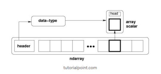
It creates an ndarray from any object exposing array interface, or from any method that returns an array.

numpy.array(object, dtype = None, copy = True, order = None, subok = False, ndmin = 0)

The above constructor takes the following parameters −

Object :- Any object exposing the array interface method returns an array, or any (nested) sequence.

Dtype : — Desired data type of array, optional.

Copy :- Optional. By default (true), the object is copied.

Order :- C (row major) or F (column major) or A (any) (default).

Subok :- By default, returned array forced to be a base class array. If true, sub-classes passed through.

ndmin :- Specifies minimum dimensions of resultant array.

Operations on Numpy Array

In this blog, we’ll walk through using NumPy to analyze data on wine quality. The data contains information on various attributes of wines, such as pH and fixed acidity, along with a quality score between 0 and 10 for each wine. The quality score is the average of at least 3 human taste testers. As we learn how to work with NumPy, we’ll try to figure out more about the perceived quality of wine.

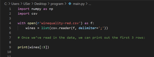
The data was downloaded from the winequality-red.csv, and is available here. file, which we’ll be using throughout this tutorial:

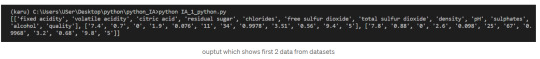
Lists Of Lists for CSV Data

Before using NumPy, we’ll first try to work with the data using Python and the csv package. We can read in the file using the csv.reader object, which will allow us to read in and split up all the content from the ssv file.

In the below code, we:

Import the csv library.

Open the winequality-red.csv file.

With the file open, create a new csv.reader object.

Pass in the keyword argument delimiter=";" to make sure that the records are split up on the semicolon character instead of the default comma character.

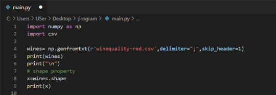
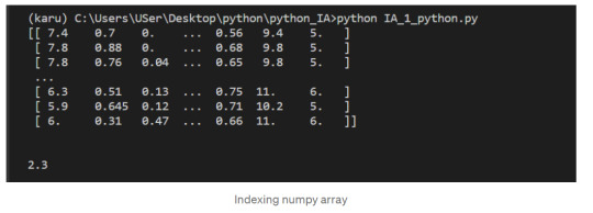
Call the list type to get all the rows from the file.

Assign the result to wines.

We can check the number of rows and columns in our data using the shape property of NumPy arrays:

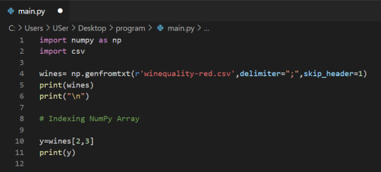
Indexing NumPy Arrays

Let’s select the element at row 3 and column 4. In the below code, we pass in the index 2 as the row index, and the index 3 as the column index. This retrieves the value from the fourth column of the third row:

1-Dimensional NumPy Arrays

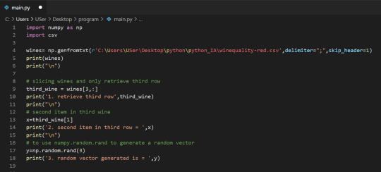
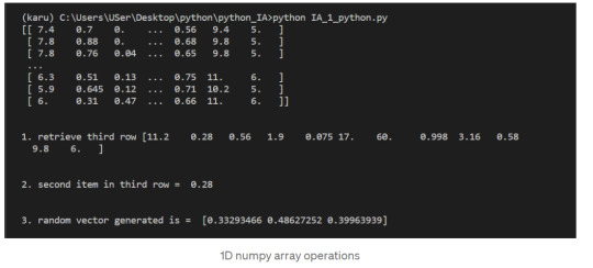
So far, we’ve worked with 2-dimensional arrays, such as wines. However, NumPy is a package for working with multidimensional arrays. One of the most common types of multidimensional arrays is the 1-dimensional array, or vector.

1.Just like a list of lists is analogous to a 2-dimensional array, a single list is analogous to a 1-dimensional array. If we slice wines and only retrieve the third row, we get a 1-dimensional array:

2. We can retrieve individual elements from third_wine using a single index. The below code will display the second item in third_wine:

3. Most NumPy functions that we’ve worked with, such as numpy.random.rand, can be used with multidimensional arrays. Here’s how we’d use numpy.random.rand to generate a random vector:

After successfully reading our dataset and learning about List, Indexing, & 1D array in NumPy we can start performing the operation on it.

The first element of each row is the fixed acidity, the second is the volatile ,acidity, and so on. We can find the average quality of the wines. The below code will:

Extract the last element from each row after the header row.

Convert each extracted element to a float.

Assign all the extracted elements to the list qualities.

Divide the sum of all the elements in qualities by the total number of elements in qualities to the get the mean.

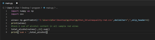
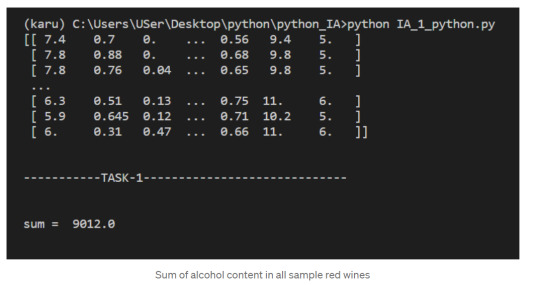
NumPy Array Methods

In addition to the common mathematical operations, NumPy also has several methods that you can use for more complex calculations on arrays. An example of this is the numpy.ndarray.sum method. This finds the sum of all the elements in an array by default:

2. Sum of alcohol content in all sample red wines

NumPy Array Comparisons

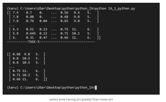
We get a Boolean array that tells us which of the wines have a quality rating greater than 5. We can do something similar with the other operators. For instance, we can see if any wines have a quality rating equal to 10:

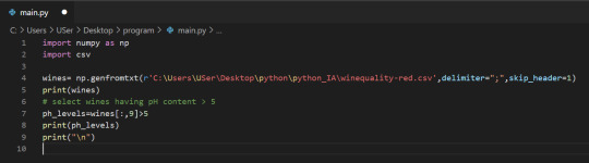
3. select wines having pH content > 5

Subsetting

We select only the rows where high_Quality contains a True value, and all of the columns. This subsetting makes it simple to filter arrays for certain criteria. For example, we can look for wines with a lot of alcohol and high quality. In order to specify multiple conditions, we have to place each condition in parentheses, and separate conditions with an ampersand (&):

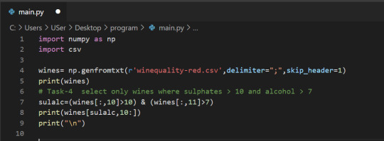
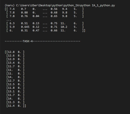
4. Select only wines where sulphates >10 and alcohol >7

5. select wine having pH greater than mean pH

We have seen what NumPy is, and some of its most basic uses. In the following posts we will see more complex functionalities and dig deeper into the workings of this fantastic library!

To check it out follow me on tumblr, and stay tuned!

That is all, I hope you liked the post. Feel Free to follow me on tumblr

Also, you can take a look at my other posts on Data Science and Machine Learning here. Have a good read!

[usmanshami-blog]

Trying out AWS SageMaker Studio for a simple machine learning task

Overview

Let’s look at how to accomplish a simple machine learning task on

AWS SageMaker

We'll take a movie ratings dataset comprising of user ratings for different movies and the movie metadata. Based on these existing user ratings of different movies, we'll try to predict what the user's rating would be for a movie that they haven't rated yet.  

The following two documents are the primary references used in creating this doc - so feel free to refer to them in case there are any issues.

[1] Build, Train, and Deploy a Machine Learning Model (https://aws.amazon.com/getting-started/hands-on/build-train-deploy-machine-learning-model-sagemaker/) [2] Machine Learning Project – Data Science Movie Recommendation System Project in R (https://data-flair.training/blogs/data-science-r-movie-recommendation/)

We'd be using the MovieLens data from GroupLens Research.

[3] MovieLens | GroupLens (https://grouplens.org/datasets/movielens/)

Steps

Log into the AWS console and select Amazon SageMaker from the services to be redirected to the SageMaker Dashboard.

Select Amazon SageMaker Studio from the navigation bar on the left and select quick start to start a new instance of Amazon SageMaker Studio. Consider leaving the default name as is, select "Create a new role" in execution role and specify the S3 buckets you'd be using (Leaving these defaults should be okay as well) and click "Create Role". Once the execution role has been created, click on “Submit” - this will create a new Amazon SageMaker instance.

Once the Amazon SageMaker Studio instance is created, click on Open Studio link to launch the Amazon SageMaker Studio IDE.

Create a new Jupyter notebook using the Data Science as the Kernel and the latest python (Python 3) notebook.

Import the python libraries we'd be using in this task - boto3 is the python library which is used for making AWS requests, sagemaker is the sagemaker library and urllib.request is the library to make url requests such as HTTP GET etc to download csv files stored on S3 and elsewhere. numpy is a scientific computing python library and pandas is a python data analysis library. After writing the following code in the Jupyter notebook cell, look for a play button in the controls bar on top - click it should run the currently active cell and execute its code.    

import boto3, sagemaker, urllib.request from sagemaker import get_execution_role import numpy as np                                 import pandas as pd                               from sagemaker.predictor import csv_serializer 

Once the imports have been completed, lets add some standard code to create execution role, define region settings and initialize boto for the region and xgboost

# Define IAM role role = get_execution_role() prefix = 'sagemaker/movielens' containers = {'us-west-2': '433757028032.dkr.ecr.us-west-2.amazonaws.com/xgboost:latest',              'us-east-1': '811284229777.dkr.ecr.us-east-1.amazonaws.com/xgboost:latest',              'us-east-2': '825641698319.dkr.ecr.us-east-2.amazonaws.com/xgboost:latest',              'eu-west-1': '685385470294.dkr.ecr.eu-west-1.amazonaws.com/xgboost:latest'} # each region has its XGBoost container my_region = boto3.session.Session().region_name # set the region of the instance print("Success - the MySageMakerInstance is in the " + my_region + " region. You will use the " + containers[my_region] + " container for your SageMaker endpoint.")

Create an S3 bucket that will contain our dataset files as well as training, test data, the computed machine learning models and the results. 

bucket_name = '<BUCKET_NAME_HERE>' s3 = boto3.resource('s3') try:    if  my_region == 'us-east-1':      s3.create_bucket(Bucket=bucket_name)    else:      s3.create_bucket(Bucket=bucket_name, CreateBucketConfiguration={ 'LocationConstraint': my_region })    print('S3 bucket created successfully') except Exception as e:    print('S3 error: ',e)

Once the bucket has been created, upload the movie lens data files to the bucket by using the S3 console UI. You'll need to download the zip from https://grouplens.org/datasets/movielens/, extract it on the local machine and then upload the extracted files on S3. We used the Small dataset which has 100,000 ratings applied to 9,000 movies by 600 users. Be sure to read the MovieLens README file to make sure you understand the conditions on the data usage.  

After the files have been uploaded, add the following code to the notebook to download the csv files and convert them to pandas data format

try:  urllib.request.urlretrieve ("https://{}.s3.{}.amazonaws.com/ratings.csv".format(bucket_name, my_region), "ratings.csv")  print('Success: downloaded ratings.csv.') except Exception as e:  print('Data load error: ',e) try:  urllib.request.urlretrieve ("https://{}.s3.{}.amazonaws.com/movies.csv".format(bucket_name, my_region), "movies.csv")  print('Success: downloaded ratings.csv.') except Exception as e:  print('Data load error: ',e)

try:  model_data = pd.read_csv('./ratings.csv')  print('Success: Data loaded into dataframe.') except Exception as e:    print('Data load error: ',e) try:  movie_data = pd.read_csv('./movies.csv')  print('Success: Data loaded into dataframe.') except Exception as e:    print('Data load error: ',e)

Now we create training and test datasets from the ratings data by splitting 70-30% the data randomly

train_data, test_data = np.split(model_data.sample(frac=1, random_state=1729), [int(0.7 * len(model_data))]) print(train_data.shape, test_data.shape) print(train_data.info, test_data.info)

We will need to normalize the training and test datasets to include boolean genre membership columns for each genre. To do this, we first process the movie dataset to create a movie to list of its genres map. Once the map has been created, we iterate the ratings data and update each row with the boolean genre membership columns. The following code creates the movie genre maps

movie_id_genre_map=dict() for movie_row in movie_data.itertuples():    # print (movie_row)    genres=movie_row[3].split('|')    # print(movie_row[1])    if movie_row[1] in movie_id_genre_map:        raise    movie_id_genre_map[movie_row[1]] = genres

print(len(movie_id_genre_map))

We now normalize the training data as mentioned above. Note that the rating column which is the column we are trying to predict in this model (and would be classifying into different rating classes) needs to be the first column in the training dataset. Also note that we multiplied the rating with 2 to convert it from 0.5-5 range of 0.5 rating increments to the range of 1-10. This is necessary since the new integer rating value becomes the rating class for the model classification.  

normalized_train_data = list() for tuple in train_data.itertuples():    userId = tuple[1]    movieId = tuple[2]    rating = tuple[3]/0.5    timestamp = tuple[4]    curr_row_normalized=dict()    curr_row_normalized['rating'] = rating    curr_row_normalized['userId'] = userId    curr_row_normalized['movieId'] = movieId    curr_row_normalized['timestamp'] = timestamp    curr_genres = {'Action': 0,     'Adventure': 0,     'Animation': 0,     'Children': 0,     'Comedy': 0,     'Crime': 0,     'Documentary': 0,     'Drama': 0,     'Fantasy': 0,     'Film-Noir': 0,     'Horror': 0,     'Musical': 0,     'Mystery': 0,     'Romance': 0,     'Sci-Fi': 0,     'Thriller': 0,     'War': 0,     'Western': 0    }    curr_movie = movie_id_genre_map[movieId]    for genre in curr_movie:        curr_genres[genre]=1

   curr_row_normalized.update(curr_genres)    normalized_train_data.append(curr_row_normalized)    #print(curr_row_normalized)    #print(normalized_train_data)

print(len(normalized_train_data)) normalized_train_data_pd = pd.DataFrame(data=normalized_train_data) print(normalized_train_data_pd.columns)

We do the same for test data, with a small difference - we create two different normalized data arrays - one with the user's rating and one without the user's rating. The one without the user's rating would be used in ML predictions - and these predictions would then be compared with the array with user's ratings to determine the accuracy of the predictions.

normalized_test_data = list() normalized_test_data_array = list() for tuple in test_data.itertuples():    userId = tuple[1]    movieId = tuple[2]    rating = tuple[3]/0.5    timestamp = tuple[4]    curr_array_row_normalized=dict()    curr_row_normalized=dict()    curr_row_normalized['rating'] = rating    curr_row_normalized['userId'] = userId    curr_array_row_normalized['userId'] = userId    curr_row_normalized['movieId'] = movieId    curr_array_row_normalized['movieId'] = movieId    curr_row_normalized['timestamp'] = timestamp    curr_array_row_normalized['timestamp'] = timestamp    curr_genres = {'Action': 0,     'Adventure': 0,     'Animation': 0,     'Children': 0,     'Comedy': 0,     'Crime': 0,     'Documentary': 0,     'Drama': 0,     'Fantasy': 0,     'Film-Noir': 0,     'Horror': 0,     'Musical': 0,     'Mystery': 0,     'Romance': 0,     'Sci-Fi': 0,     'Thriller': 0,     'War': 0,     'Western': 0    }    curr_movie = movie_id_genre_map[movieId]    for genre in curr_movie:        curr_genres[genre]=1

   curr_row_normalized.update(curr_genres)    curr_array_row_normalized.update(curr_genres)    normalized_test_data.append(curr_row_normalized)    normalized_test_data_array.append(curr_array_row_normalized)    #print(curr_row_normalized)    #print(normalized_test_data) print(len(normalized_test_data)) print(len(normalized_test_data_array)) normalized_test_data_pd = pd.DataFrame(data=normalized_test_data) print(normalized_test_data_pd.columns) normalized_test_data_array_pd = pd.DataFrame(data=normalized_test_data_array) print(normalized_test_data_array_pd.columns)

Now lets run the predictions

xgb_predictor.content_type = 'text/csv' xgb_predictor.serializer = csv_serializer predictions = xgb_predictor.predict(normalized_test_data_array_pd.values).decode('utf-8') predictions_array = np.fromstring(predictions[1:], sep=',') # and turn the prediction into an array print(predictions_array)

Now create a frequency histogram of the rating classes for the predictions array - pandas crosstab utility does the trick here

cm = pd.crosstab(index=normalized_test_data_pd['rating'], columns=np.round(predictions_array), rownames=['Observed'], colnames=['Predicted'])

Now compute the accuracy of the prediction - we define the following classes - zero distance i.e. the prediction was accurate, one distance i.e. the predicted score differed from the actual by 1, two distance i.e. the predicted score differed from the actual by 2 and remaining i.e. the predicted score differed from actual by > 2

zero_distance = 0 one_distance = 0 two_distance = 0 remaining = 0 total = 0 for tuple in cm.itertuples():    total += tuple[0]    total += tuple[1]    total += tuple[2]    total += tuple[3]    total += tuple[4]    total += tuple[5]    total += tuple[6]    total += tuple[7]    total += tuple[8]    total += tuple[9]    total += tuple[10]

   actual = tuple[0]    if actual == 1.0:        zero_distance += tuple[1]        one_distance += tuple[2]        two_distance += tuple[3]        remaining += tuple[4]        remaining += tuple[5]        remaining += tuple[6]        remaining += tuple[7]        remaining += tuple[8]        remaining += tuple[9]        remaining += tuple[10]

   if actual == 2.0:        zero_distance += tuple[2]        one_distance += tuple[1]        one_distance += tuple[3]        two_distance += tuple[4]        remaining += tuple[5]        remaining += tuple[6]        remaining += tuple[7]        remaining += tuple[8]        remaining += tuple[9]        remaining += tuple[10]

   if actual == 3.0:        zero_distance += tuple[3]        one_distance += tuple[2]        one_distance += tuple[4]        two_distance += tuple[1]        two_distance += tuple[5]        remaining += tuple[6]        remaining += tuple[7]        remaining += tuple[8]        remaining += tuple[9]        remaining += tuple[10]

   if actual == 4.0:        zero_distance += tuple[4]        one_distance += tuple[3]        one_distance += tuple[5]        two_distance += tuple[2]        two_distance += tuple[6]        remaining += tuple[1]        remaining += tuple[7]        remaining += tuple[8]        remaining += tuple[9]        remaining += tuple[10]

   if actual == 5.0:        zero_distance += tuple[5]        one_distance += tuple[4]        one_distance += tuple[6]        two_distance += tuple[3]        two_distance += tuple[7]        remaining += tuple[1]        remaining += tuple[2]        remaining += tuple[8]        remaining += tuple[9]        remaining += tuple[10]

   if actual == 6.0:        zero_distance += tuple[6]        one_distance += tuple[5]        one_distance += tuple[7]        two_distance += tuple[4]        two_distance += tuple[8]        remaining += tuple[1]        remaining += tuple[2]        remaining += tuple[3]        remaining += tuple[9]        remaining += tuple[10]

   if actual == 7.0:        zero_distance += tuple[7]        one_distance += tuple[6]        one_distance += tuple[8]        two_distance += tuple[5]        two_distance += tuple[9]        remaining += tuple[1]        remaining += tuple[2]        remaining += tuple[3]        remaining += tuple[4]        remaining += tuple[10]

   if actual == 8.0:        zero_distance += tuple[8]        one_distance += tuple[7]        one_distance += tuple[9]        two_distance += tuple[6]        two_distance += tuple[10]        remaining += tuple[1]        remaining += tuple[2]        remaining += tuple[3]        remaining += tuple[4]        remaining += tuple[5]

   if actual == 9.0:        zero_distance += tuple[9]        one_distance += tuple[8]        one_distance += tuple[10]        two_distance += tuple[7]        remaining += tuple[1]        remaining += tuple[2]        remaining += tuple[3]        remaining += tuple[4]        remaining += tuple[5]        remaining += tuple[6]

   if actual == 10.0:        zero_distance += tuple[10]        one_distance += tuple[9]        two_distance += tuple[8]        remaining += tuple[1]        remaining += tuple[2]        remaining += tuple[3]        remaining += tuple[4]        remaining += tuple[5]        remaining += tuple[6]        remaining += tuple[7]

zero_distance_percent = 100*(zero_distance/total) one_distance_percent = 100*(one_distance/total) two_distance_percent = 100*(two_distance/total) remaining_percent = 100*(remaining/total) print("zero distance percentage: "+str(zero_distance_percent)) print("one distance percentage: "+str(one_distance_percent)) print("two distance percentage: "+str(two_distance_percent)) print("remaining distance percentage: "+str(remaining_percent))

The results show that our model was 100% accurate for 11.4% predictions, had a deviation of 1 for 47.64% predictions, deviation of 2 for 13.51% predictions and deviation of > 2 for the remaining 27.24%

zero distance percentage: 11.403445800430726 one distance percentage: 47.641780330222545 two distance percentage: 13.513998564249821 remaining distance percentage: 27.243359655419958

Now terminate the sagemaker instance and free the allocated resources.

sagemaker.Session().delete_endpoint(xgb_predictor.endpoint) bucket_to_delete = boto3.resource('s3').Bucket(bucket_name) bucket_to_delete.objects.all().delete()

[craigbrownphd]

If you did not already know

SenGen We present a new topic model that generates documents by sampling a topic for one whole sentence at a time, and generating the words in the sentence using an RNN decoder that is conditioned on the topic of the sentence. We argue that this novel formalism will help us not only visualize and model the topical discourse structure in a document better, but also potentially lead to more interpretable topics since we can now illustrate topics by sampling representative sentences instead of bag of words or phrases. We present a variational auto-encoder approach for learning in which we use a factorized variational encoder that independently models the posterior over topical mixture vectors of documents using a feed-forward network, and the posterior over topic assignments to sentences using an RNN. Our preliminary experiments on two different datasets indicate early promise, but also expose many challenges that remain to be addressed. … In-Database Entity Linking (IDEL) We present a novel architecture, In-Database Entity Linking (IDEL), in which we integrate the analytics-optimized RDBMS MonetDB with neural text mining abilities. Our system design abstracts core tasks of most neural entity linking systems for MonetDB. To the best of our knowledge, this is the first defacto implemented system integrating entity-linking in a database. We leverage the ability of MonetDB to support in-database-analytics with user defined functions (UDFs) implemented in Python. These functions call machine learning libraries for neural text mining, such as TensorFlow. The system achieves zero cost for data shipping and transformation by utilizing MonetDB’s ability to embed Python processes in the database kernel and exchange data in NumPy arrays. IDEL represents text and relational data in a joint vector space with neural embeddings and can compensate errors with ambiguous entity representations. For detecting matching entities, we propose a novel similarity function based on joint neural embeddings which are learned via minimizing pairwise contrastive ranking loss. This function utilizes a high dimensional index structures for fast retrieval of matching entities. Our first implementation and experiments using the WebNLG corpus show the effectiveness and the potentials of IDEL. … REINFORCEjs REINFORCEjs is a Reinforcement Learning library that implements several common RL algorithms, all with web demos. In particular, the library currently includes: · Dynamic Programming methods · (Tabular) Temporal Difference Learning (SARSA/Q-Learning) · Deep Q-Learning for Q-Learning with function approximation with Neural Networks · Stochastic/Deterministic Policy Gradients and Actor Critic architectures for dealing with continuous action spaces. (very alpha, likely buggy or at the very least finicky and inconsistent) GitHub REINFORCEjs … RRDtool RRDtool (round-robin database tool) aims to handle time series data such as network bandwidth, temperatures or CPU load. The data is stored in a circular buffer based database, thus the system storage footprint remains constant over time. RRDtool … https://analytixon.com/2023/04/09/if-you-did-not-already-know-2013/?utm_source=dlvr.it&utm_medium=tumblr

[python-syntax-cheat-sheeteg]

python syntax cheat sheet working 0T0&

💾 ►►► DOWNLOAD FILE 🔥🔥🔥🔥🔥 int() → 15 truncate decimal part float("e8") → round(,1)→ rounding to 1 decimal (0 decimal → integer number). It's easy to learn and fun, and its syntax is simple yet elegant. Python is a popular choice for beginners, yet still powerful enough to to back some of the. Python CheatSheet. Basic syntax from the python programming language. Showing Output To User. The print function is used to display or print output. Basic rules to write Python syntax: Rule #1: Python is white-space dependent; code blocks are indented using spaces. Rule #2: Python language. 9 Work fast with our official CLI. Learn more. If nothing happens, download GitHub Desktop and try again. If nothing happens, download Xcode and try again. There was a problem preparing your codespace, please try again. Each abstract base class specifies a set of virtual subclasses. These classes are then recognized by isinstance and issubclass as subclasses of the ABC, although they are really not. ABC can also manually decide whether or not a specific class is its virtual subclass, usually based on which methods the class has implemented. Splat expands a collection into positional arguments, while splatty-splat expands a dictionary into keyword arguments. Splat combines zero or more positional arguments into a tuple, while splatty-splat combines zero or more keyword arguments into a dictionary. If variable is being assigned to anywhere in the scope, it is regarded as a local variable, unless it is declared as a 'global' or a 'nonlocal'. Decorator that prints function's name every time the function is called. Decorator that caches function's return values. All function's arguments must be hashable. A decorator that accepts arguments and returns a normal decorator that accepts a function. MRO determines the order in which parent classes are traversed when searching for a method or an attribute:. Decorator that automatically generates init , repr and eq special methods. Mechanism that restricts objects to attributes listed in 'slots' and significantly reduces their memory footprint. A duck type is an implicit type that prescribes a set of special methods. Any object that has those methods defined is considered a member of that duck type. Unlike listdir , scandir returns DirEntry objects that cache isfile, isdir and on Windows also stat information, thus significantly increasing the performance of code that requires it. A server-less database engine that stores each database into a separate file. Values are not actually saved in this example because 'conn. Bytes object is an immutable sequence of single bytes. Mutable version is called bytearray. List that can only hold numbers of a predefined type. Available types and their minimum sizes in bytes are listed above. Sizes and byte order are always determined by the system. A thread-safe list with efficient appends and pops from either side. Pronounced "deck". Type is the root class. If only passed an object it returns its type class. Otherwise it creates a new class. Right before a class is created it checks if it has the 'metaclass' attribute defined. If not, it recursively checks if any of his parents has it defined and eventually comes to type. Exception description, stack trace and values of variables are appended automatically. Array manipulation mini-language. It can run up to one hundred times faster than the equivalent Python code. Object that groups together rows of a dataframe based on the value of the passed column. Skip to content. Star Comprehensive Python Cheatsheet gto This commit does not belong to any branch on this repository, and may belong to a fork outside of the repository. Branches Tags. Could not load branches. Could not load tags. Launching Xcode If nothing happens, download Xcode and try again. Launching Visual Studio Code Your codespace will open once ready. Latest commit. Git stats 2, commits. Failed to load latest commit information. Oct 2, View code. Use a capital letter for unsigned type. If array shapes differ in length, left-pad the shorter shape with ones: 2. If any dimensions differ in size, expand the ones that have size 1 by duplicating their elements: 3. If neither non-matching dimension has size 1, raise an error. Example For each point returns index of its nearest point [0. Contents 1. Also works on strings. Also works on dictionary and set. Replaces ones with matching keys. Accepts floats. Indices can be None. Fraction yes yes yes yes float yes yes yes complex yes yes decimal. Also group 0. London without DST. Also gettz. Raises ValueError. Could be too late to start deleting vars. Do not mix. Joins two or more pathname components. Also Path '. Also Path. Permissions are in octal. Returns its stdout pipe. Returns None on success. Also ':memory:'. Exits the block with commit or rollback. A multithreaded and non-lazy map. Starts a thread and returns its Future object. Full exception if full. Empty exception if empty. Also locals. BeautifulSoup html , 'html. ConnectionError : print "You've got problems with connection. Last point gets connected to the first. Draw frame draw. Rect , , 20 , 20 while all event. QUIT for event in pg. Rect x , y , width , height Floats get truncated into ints. Allows assignments. Surface width , height New RGB surface. Format depends on source. Pass None for default. BytesIO urllib. Clock while all event. Also plt. Sr is treated as a row. Uses 'left' by default. Use l. A Series is c. Also updates b 3 4 5 items that contain NaN. Func can return DF, Sr or el. All operations return a Sr. Text "What's your name? Input ], [ sg. About Comprehensive Python Cheatsheet gto Contributors You signed in with another tab or window. Reload to refresh your session. You signed out in another tab or window.