#how to use zeros array python numpy
Explore tagged Tumblr posts
Visit Tumblr Blog
Explore Tumblr blogs with no restrictions, modern design and the best experience.
Last Seen Tumblr Blogs


Fun Fact
Tumblr has been banned in Indonesia for providing people with access to pornographic content.
Text
25 Udemy Paid Courses for Free with Certification (Only for Limited Time)

2023 Complete SQL Bootcamp from Zero to Hero in SQL
Become an expert in SQL by learning through concept & Hands-on coding :)
What you'll learn
Use SQL to query a database Be comfortable putting SQL on their resume Replicate real-world situations and query reports Use SQL to perform data analysis Learn to perform GROUP BY statements Model real-world data and generate reports using SQL Learn Oracle SQL by Professionally Designed Content Step by Step! Solve any SQL-related Problems by Yourself Creating Analytical Solutions! Write, Read and Analyze Any SQL Queries Easily and Learn How to Play with Data! Become a Job-Ready SQL Developer by Learning All the Skills You will Need! Write complex SQL statements to query the database and gain critical insight on data Transition from the Very Basics to a Point Where You can Effortlessly Work with Large SQL Queries Learn Advanced Querying Techniques Understand the difference between the INNER JOIN, LEFT/RIGHT OUTER JOIN, and FULL OUTER JOIN Complete SQL statements that use aggregate functions Using joins, return columns from multiple tables in the same query
Enroll Now 👇👇👇👇👇👇👇 https://www.book-somahar.com/2023/10/25-udemy-paid-courses-for-free-with.html
Python Programming Complete Beginners Course Bootcamp 2023
2023 Complete Python Bootcamp || Python Beginners to advanced || Python Master Class || Mega Course
What you'll learn
Basics in Python programming Control structures, Containers, Functions & Modules OOPS in Python How python is used in the Space Sciences Working with lists in python Working with strings in python Application of Python in Mars Rovers sent by NASA
Enroll Now 👇👇👇👇👇👇👇 https://www.book-somahar.com/2023/10/25-udemy-paid-courses-for-free-with.html
Learn PHP and MySQL for Web Application and Web Development
Unlock the Power of PHP and MySQL: Level Up Your Web Development Skills Today
What you'll learn
Use of PHP Function Use of PHP Variables Use of MySql Use of Database
Enroll Now 👇👇👇👇👇👇👇 https://www.book-somahar.com/2023/10/25-udemy-paid-courses-for-free-with.html
T-Shirt Design for Beginner to Advanced with Adobe Photoshop
Unleash Your Creativity: Master T-Shirt Design from Beginner to Advanced with Adobe Photoshop
What you'll learn
Function of Adobe Photoshop Tools of Adobe Photoshop T-Shirt Design Fundamentals T-Shirt Design Projects
Enroll Now 👇👇👇👇👇👇👇 https://www.book-somahar.com/2023/10/25-udemy-paid-courses-for-free-with.html
Complete Data Science BootCamp
Learn about Data Science, Machine Learning and Deep Learning and build 5 different projects.
What you'll learn
Learn about Libraries like Pandas and Numpy which are heavily used in Data Science. Build Impactful visualizations and charts using Matplotlib and Seaborn. Learn about Machine Learning LifeCycle and different ML algorithms and their implementation in sklearn. Learn about Deep Learning and Neural Networks with TensorFlow and Keras Build 5 complete projects based on the concepts covered in the course.
Enroll Now 👇👇👇👇👇👇👇 https://www.book-somahar.com/2023/10/25-udemy-paid-courses-for-free-with.html
Essentials User Experience Design Adobe XD UI UX Design
Learn UI Design, User Interface, User Experience design, UX design & Web Design
What you'll learn
How to become a UX designer Become a UI designer Full website design All the techniques used by UX professionals
Enroll Now 👇👇👇👇👇👇👇 https://www.book-somahar.com/2023/10/25-udemy-paid-courses-for-free-with.html
Build a Custom E-Commerce Site in React + JavaScript Basics
Build a Fully Customized E-Commerce Site with Product Categories, Shopping Cart, and Checkout Page in React.
What you'll learn
Introduction to the Document Object Model (DOM) The Foundations of JavaScript JavaScript Arithmetic Operations Working with Arrays, Functions, and Loops in JavaScript JavaScript Variables, Events, and Objects JavaScript Hands-On - Build a Photo Gallery and Background Color Changer Foundations of React How to Scaffold an Existing React Project Introduction to JSON Server Styling an E-Commerce Store in React and Building out the Shop Categories Introduction to Fetch API and React Router The concept of "Context" in React Building a Search Feature in React Validating Forms in React
Enroll Now 👇👇👇👇👇👇👇 https://www.book-somahar.com/2023/10/25-udemy-paid-courses-for-free-with.html
Complete Bootstrap & React Bootcamp with Hands-On Projects
Learn to Build Responsive, Interactive Web Apps using Bootstrap and React.
What you'll learn
Learn the Bootstrap Grid System Learn to work with Bootstrap Three Column Layouts Learn to Build Bootstrap Navigation Components Learn to Style Images using Bootstrap Build Advanced, Responsive Menus using Bootstrap Build Stunning Layouts using Bootstrap Themes Learn the Foundations of React Work with JSX, and Functional Components in React Build a Calculator in React Learn the React State Hook Debug React Projects Learn to Style React Components Build a Single and Multi-Player Connect-4 Clone with AI Learn React Lifecycle Events Learn React Conditional Rendering Build a Fully Custom E-Commerce Site in React Learn the Foundations of JSON Server Work with React Router
Enroll Now 👇👇👇👇👇👇👇 https://www.book-somahar.com/2023/10/25-udemy-paid-courses-for-free-with.html
Build an Amazon Affiliate E-Commerce Store from Scratch
Earn Passive Income by Building an Amazon Affiliate E-Commerce Store using WordPress, WooCommerce, WooZone, & Elementor
What you'll learn
Registering a Domain Name & Setting up Hosting Installing WordPress CMS on Your Hosting Account Navigating the WordPress Interface The Advantages of WordPress Securing a WordPress Installation with an SSL Certificate Installing Custom Themes for WordPress Installing WooCommerce, Elementor, & WooZone Plugins Creating an Amazon Affiliate Account Importing Products from Amazon to an E-Commerce Store using WooZone Plugin Building a Customized Shop with Menu's, Headers, Branding, & Sidebars Building WordPress Pages, such as Blogs, About Pages, and Contact Us Forms Customizing Product Pages on a WordPress Power E-Commerce Site Generating Traffic and Sales for Your Newly Published Amazon Affiliate Store
Enroll Now 👇👇👇👇👇👇👇 https://www.book-somahar.com/2023/10/25-udemy-paid-courses-for-free-with.html
The Complete Beginner Course to Optimizing ChatGPT for Work
Learn how to make the most of ChatGPT's capabilities in efficiently aiding you with your tasks.
What you'll learn
Learn how to harness ChatGPT's functionalities to efficiently assist you in various tasks, maximizing productivity and effectiveness. Delve into the captivating fusion of product development and SEO, discovering effective strategies to identify challenges, create innovative tools, and expertly Understand how ChatGPT is a technological leap, akin to the impact of iconic tools like Photoshop and Excel, and how it can revolutionize work methodologies thr Showcase your learning by creating a transformative project, optimizing your approach to work by identifying tasks that can be streamlined with artificial intel
Enroll Now 👇👇👇👇👇👇👇 https://www.book-somahar.com/2023/10/25-udemy-paid-courses-for-free-with.html
AWS, JavaScript, React | Deploy Web Apps on the Cloud
Cloud Computing | Linux Foundations | LAMP Stack | DBMS | Apache | NGINX | AWS IAM | Amazon EC2 | JavaScript | React
What you'll learn
Foundations of Cloud Computing on AWS and Linode Cloud Computing Service Models (IaaS, PaaS, SaaS) Deploying and Configuring a Virtual Instance on Linode and AWS Secure Remote Administration for Virtual Instances using SSH Working with SSH Key Pair Authentication The Foundations of Linux (Maintenance, Directory Commands, User Accounts, Filesystem) The Foundations of Web Servers (NGINX vs Apache) Foundations of Databases (SQL vs NoSQL), Database Transaction Standards (ACID vs CAP) Key Terminology for Full Stack Development and Cloud Administration Installing and Configuring LAMP Stack on Ubuntu (Linux, Apache, MariaDB, PHP) Server Security Foundations (Network vs Hosted Firewalls). Horizontal and Vertical Scaling of a virtual instance on Linode using NodeBalancers Creating Manual and Automated Server Images and Backups on Linode Understanding the Cloud Computing Phenomenon as Applicable to AWS The Characteristics of Cloud Computing as Applicable to AWS Cloud Deployment Models (Private, Community, Hybrid, VPC) Foundations of AWS (Registration, Global vs Regional Services, Billing Alerts, MFA) AWS Identity and Access Management (Mechanics, Users, Groups, Policies, Roles) Amazon Elastic Compute Cloud (EC2) - (AMIs, EC2 Users, Deployment, Elastic IP, Security Groups, Remote Admin) Foundations of the Document Object Model (DOM) Manipulating the DOM Foundations of JavaScript Coding (Variables, Objects, Functions, Loops, Arrays, Events) Foundations of ReactJS (Code Pen, JSX, Components, Props, Events, State Hook, Debugging) Intermediate React (Passing Props, Destrcuting, Styling, Key Property, AI, Conditional Rendering, Deployment) Building a Fully Customized E-Commerce Site in React Intermediate React Concepts (JSON Server, Fetch API, React Router, Styled Components, Refactoring, UseContext Hook, UseReducer, Form Validation)
Enroll Now 👇👇👇👇👇👇👇 https://www.book-somahar.com/2023/10/25-udemy-paid-courses-for-free-with.html
Run Multiple Sites on a Cloud Server: AWS & Digital Ocean
Server Deployment | Apache Configuration | MySQL | PHP | Virtual Hosts | NS Records | DNS | AWS Foundations | EC2
What you'll learn
A solid understanding of the fundamentals of remote server deployment and configuration, including network configuration and security. The ability to install and configure the LAMP stack, including the Apache web server, MySQL database server, and PHP scripting language. Expertise in hosting multiple domains on one virtual server, including setting up virtual hosts and managing domain names. Proficiency in virtual host file configuration, including creating and configuring virtual host files and understanding various directives and parameters. Mastery in DNS zone file configuration, including creating and managing DNS zone files and understanding various record types and their uses. A thorough understanding of AWS foundations, including the AWS global infrastructure, key AWS services, and features. A deep understanding of Amazon Elastic Compute Cloud (EC2) foundations, including creating and managing instances, configuring security groups, and networking. The ability to troubleshoot common issues related to remote server deployment, LAMP stack installation and configuration, virtual host file configuration, and D An understanding of best practices for remote server deployment and configuration, including security considerations and optimization for performance. Practical experience in working with remote servers and cloud-based solutions through hands-on labs and exercises. The ability to apply the knowledge gained from the course to real-world scenarios and challenges faced in the field of web hosting and cloud computing. A competitive edge in the job market, with the ability to pursue career opportunities in web hosting and cloud computing.
Enroll Now 👇👇👇👇👇👇👇 https://www.book-somahar.com/2023/10/25-udemy-paid-courses-for-free-with.html
Cloud-Powered Web App Development with AWS and PHP
AWS Foundations | IAM | Amazon EC2 | Load Balancing | Auto-Scaling Groups | Route 53 | PHP | MySQL | App Deployment
What you'll learn
Understanding of cloud computing and Amazon Web Services (AWS) Proficiency in creating and configuring AWS accounts and environments Knowledge of AWS pricing and billing models Mastery of Identity and Access Management (IAM) policies and permissions Ability to launch and configure Elastic Compute Cloud (EC2) instances Familiarity with security groups, key pairs, and Elastic IP addresses Competency in using AWS storage services, such as Elastic Block Store (EBS) and Simple Storage Service (S3) Expertise in creating and using Elastic Load Balancers (ELB) and Auto Scaling Groups (ASG) for load balancing and scaling web applications Knowledge of DNS management using Route 53 Proficiency in PHP programming language fundamentals Ability to interact with databases using PHP and execute SQL queries Understanding of PHP security best practices, including SQL injection prevention and user authentication Ability to design and implement a database schema for a web application Mastery of PHP scripting to interact with a database and implement user authentication using sessions and cookies Competency in creating a simple blog interface using HTML and CSS and protecting the blog content using PHP authentication. Students will gain practical experience in creating and deploying a member-only blog with user authentication using PHP and MySQL on AWS.
Enroll Now 👇👇👇👇👇👇👇 https://www.book-somahar.com/2023/10/25-udemy-paid-courses-for-free-with.html
CSS, Bootstrap, JavaScript And PHP Stack Complete Course
CSS, Bootstrap And JavaScript And PHP Complete Frontend and Backend Course
What you'll learn
Introduction to Frontend and Backend technologies Introduction to CSS, Bootstrap And JavaScript concepts, PHP Programming Language Practically Getting Started With CSS Styles, CSS 2D Transform, CSS 3D Transform Bootstrap Crash course with bootstrap concepts Bootstrap Grid system,Forms, Badges And Alerts Getting Started With Javascript Variables,Values and Data Types, Operators and Operands Write JavaScript scripts and Gain knowledge in regard to general javaScript programming concepts PHP Section Introduction to PHP, Various Operator types , PHP Arrays, PHP Conditional statements Getting Started with PHP Function Statements And PHP Decision Making PHP 7 concepts PHP CSPRNG And PHP Scalar Declaration
Enroll Now 👇👇👇👇👇👇👇 https://www.book-somahar.com/2023/10/25-udemy-paid-courses-for-free-with.html
Learn HTML - For Beginners
Lean how to create web pages using HTML
What you'll learn
How to Code in HTML Structure of an HTML Page Text Formatting in HTML Embedding Videos Creating Links Anchor Tags Tables & Nested Tables Building Forms Embedding Iframes Inserting Images
Enroll Now 👇👇👇👇👇👇👇 https://www.book-somahar.com/2023/10/25-udemy-paid-courses-for-free-with.html
Learn Bootstrap - For Beginners
Learn to create mobile-responsive web pages using Bootstrap
What you'll learn
Bootstrap Page Structure Bootstrap Grid System Bootstrap Layouts Bootstrap Typography Styling Images Bootstrap Tables, Buttons, Badges, & Progress Bars Bootstrap Pagination Bootstrap Panels Bootstrap Menus & Navigation Bars Bootstrap Carousel & Modals Bootstrap Scrollspy Bootstrap Themes
Enroll Now 👇👇👇👇👇👇👇 https://www.book-somahar.com/2023/10/25-udemy-paid-courses-for-free-with.html
JavaScript, Bootstrap, & PHP - Certification for Beginners
A Comprehensive Guide for Beginners interested in learning JavaScript, Bootstrap, & PHP
What you'll learn
Master Client-Side and Server-Side Interactivity using JavaScript, Bootstrap, & PHP Learn to create mobile responsive webpages using Bootstrap Learn to create client and server-side validated input forms Learn to interact with a MySQL Database using PHP
Enroll Now 👇👇👇👇👇👇👇 https://www.book-somahar.com/2023/10/25-udemy-paid-courses-for-free-with.html
Linode: Build and Deploy Responsive Websites on the Cloud
Cloud Computing | IaaS | Linux Foundations | Apache + DBMS | LAMP Stack | Server Security | Backups | HTML | CSS
What you'll learn
Understand the fundamental concepts and benefits of Cloud Computing and its service models. Learn how to create, configure, and manage virtual servers in the cloud using Linode. Understand the basic concepts of Linux operating system, including file system structure, command-line interface, and basic Linux commands. Learn how to manage users and permissions, configure network settings, and use package managers in Linux. Learn about the basic concepts of web servers, including Apache and Nginx, and databases such as MySQL and MariaDB. Learn how to install and configure web servers and databases on Linux servers. Learn how to install and configure LAMP stack to set up a web server and database for hosting dynamic websites and web applications. Understand server security concepts such as firewalls, access control, and SSL certificates. Learn how to secure servers using firewalls, manage user access, and configure SSL certificates for secure communication. Learn how to scale servers to handle increasing traffic and load. Learn about load balancing, clustering, and auto-scaling techniques. Learn how to create and manage server images. Understand the basic structure and syntax of HTML, including tags, attributes, and elements. Understand how to apply CSS styles to HTML elements, create layouts, and use CSS frameworks.
Enroll Now 👇👇👇👇👇👇👇 https://www.book-somahar.com/2023/10/25-udemy-paid-courses-for-free-with.html
PHP & MySQL - Certification Course for Beginners
Learn to Build Database Driven Web Applications using PHP & MySQL
What you'll learn
PHP Variables, Syntax, Variable Scope, Keywords Echo vs. Print and Data Output PHP Strings, Constants, Operators PHP Conditional Statements PHP Elseif, Switch, Statements PHP Loops - While, For PHP Functions PHP Arrays, Multidimensional Arrays, Sorting Arrays Working with Forms - Post vs. Get PHP Server Side - Form Validation Creating MySQL Databases Database Administration with PhpMyAdmin Administering Database Users, and Defining User Roles SQL Statements - Select, Where, And, Or, Insert, Get Last ID MySQL Prepared Statements and Multiple Record Insertion PHP Isset MySQL - Updating Records
Enroll Now 👇👇👇👇👇👇👇 https://www.book-somahar.com/2023/10/25-udemy-paid-courses-for-free-with.html
Linode: Deploy Scalable React Web Apps on the Cloud
Cloud Computing | IaaS | Server Configuration | Linux Foundations | Database Servers | LAMP Stack | Server Security
What you'll learn
Introduction to Cloud Computing Cloud Computing Service Models (IaaS, PaaS, SaaS) Cloud Server Deployment and Configuration (TFA, SSH) Linux Foundations (File System, Commands, User Accounts) Web Server Foundations (NGINX vs Apache, SQL vs NoSQL, Key Terms) LAMP Stack Installation and Configuration (Linux, Apache, MariaDB, PHP) Server Security (Software & Hardware Firewall Configuration) Server Scaling (Vertical vs Horizontal Scaling, IP Swaps, Load Balancers) React Foundations (Setup) Building a Calculator in React (Code Pen, JSX, Components, Props, Events, State Hook) Building a Connect-4 Clone in React (Passing Arguments, Styling, Callbacks, Key Property) Building an E-Commerce Site in React (JSON Server, Fetch API, Refactoring)
Enroll Now 👇👇👇👇👇👇👇 https://www.book-somahar.com/2023/10/25-udemy-paid-courses-for-free-with.html
Internet and Web Development Fundamentals
Learn how the Internet Works and Setup a Testing & Production Web Server
What you'll learn
How the Internet Works Internet Protocols (HTTP, HTTPS, SMTP) The Web Development Process Planning a Web Application Types of Web Hosting (Shared, Dedicated, VPS, Cloud) Domain Name Registration and Administration Nameserver Configuration Deploying a Testing Server using WAMP & MAMP Deploying a Production Server on Linode, Digital Ocean, or AWS Executing Server Commands through a Command Console Server Configuration on Ubuntu Remote Desktop Connection and VNC SSH Server Authentication FTP Client Installation FTP Uploading
Enroll Now 👇👇👇👇👇👇👇 https://www.book-somahar.com/2023/10/25-udemy-paid-courses-for-free-with.html
Linode: Web Server and Database Foundations
Cloud Computing | Instance Deployment and Config | Apache | NGINX | Database Management Systems (DBMS)
What you'll learn
Introduction to Cloud Computing (Cloud Service Models) Navigating the Linode Cloud Interface Remote Administration using PuTTY, Terminal, SSH Foundations of Web Servers (Apache vs. NGINX) SQL vs NoSQL Databases Database Transaction Standards (ACID vs. CAP Theorem) Key Terms relevant to Cloud Computing, Web Servers, and Database Systems
Enroll Now 👇👇👇👇👇👇👇 https://www.book-somahar.com/2023/10/25-udemy-paid-courses-for-free-with.html
Java Training Complete Course 2022
Learn Java Programming language with Java Complete Training Course 2022 for Beginners
What you'll learn
You will learn how to write a complete Java program that takes user input, processes and outputs the results You will learn OOPS concepts in Java You will learn java concepts such as console output, Java Variables and Data Types, Java Operators And more You will be able to use Java for Selenium in testing and development
Enroll Now 👇👇👇👇👇👇👇 https://www.book-somahar.com/2023/10/25-udemy-paid-courses-for-free-with.html
Learn To Create AI Assistant (JARVIS) With Python
How To Create AI Assistant (JARVIS) With Python Like the One from Marvel's Iron Man Movie
What you'll learn
how to create an personalized artificial intelligence assistant how to create JARVIS AI how to create ai assistant
Enroll Now 👇👇👇👇👇👇👇 https://www.book-somahar.com/2023/10/25-udemy-paid-courses-for-free-with.html
Keyword Research, Free Backlinks, Improve SEO -Long Tail Pro
LongTailPro is the keyword research service we at Coursenvy use for ALL our clients! In this course, find SEO keywords,
What you'll learn
Learn everything Long Tail Pro has to offer from A to Z! Optimize keywords in your page/post titles, meta descriptions, social media bios, article content, and more! Create content that caters to the NEW Search Engine Algorithms and find endless keywords to rank for in ALL the search engines! Learn how to use ALL of the top-rated Keyword Research software online! Master analyzing your COMPETITIONS Keywords! Get High-Quality Backlinks that will ACTUALLY Help your Page Rank!
Enroll Now 👇👇👇👇👇👇👇 https://www.book-somahar.com/2023/10/25-udemy-paid-courses-for-free-with.html
#udemy#free course#paid course for free#design#development#ux ui#xd#figma#web development#python#javascript#php#java#cloud
2 notes
·
View notes
Text
Python for Data Science: The Only Guide You Need to Get Started in 2025
Data is the lifeblood of modern business, powering decisions in healthcare, finance, marketing, sports, and more. And at the core of it all lies a powerful and beginner-friendly programming language — Python.
Whether you’re an aspiring data scientist, analyst, or tech enthusiast, learning Python for data science is one of the smartest career moves you can make in 2025.
In this guide, you’ll learn:
Why Python is the preferred language for data science
The libraries and tools you must master
A beginner-friendly roadmap
How to get started with a free full course on YouTube
Why Python is the #1 Language for Data Science
Python has earned its reputation as the go-to language for data science and here's why:
1. Easy to Learn, Easy to Use
Python’s syntax is clean, simple, and intuitive. You can focus on solving problems rather than struggling with the language itself.
2. Rich Ecosystem of Libraries
Python offers thousands of specialized libraries for data analysis, machine learning, and visualization.
3. Community and Resources
With a vibrant global community, you’ll never run out of tutorials, forums, or project ideas to help you grow.
4. Integration with Tools & Platforms
From Jupyter notebooks to cloud platforms like AWS and Google Colab, Python works seamlessly everywhere.
What You Can Do with Python in Data Science
Let’s look at real tasks you can perform using Python: TaskPython ToolsData cleaning & manipulationPandas, NumPyData visualizationMatplotlib, Seaborn, PlotlyMachine learningScikit-learn, XGBoostDeep learningTensorFlow, PyTorchStatistical analysisStatsmodels, SciPyBig data integrationPySpark, Dask
Python lets you go from raw data to actionable insight — all within a single ecosystem.
A Beginner's Roadmap to Learn Python for Data Science
If you're starting from scratch, follow this step-by-step learning path:
✅ Step 1: Learn Python Basics
Variables, data types, loops, conditionals
Functions, file handling, error handling
✅ Step 2: Explore NumPy
Arrays, broadcasting, numerical computations
✅ Step 3: Master Pandas
DataFrames, filtering, grouping, merging datasets
✅ Step 4: Visualize with Matplotlib & Seaborn
Create charts, plots, and visual dashboards
✅ Step 5: Intro to Machine Learning
Use Scikit-learn for classification, regression, clustering
✅ Step 6: Work on Real Projects
Apply your knowledge to real-world datasets (Kaggle, UCI, etc.)
Who Should Learn Python for Data Science?
Python is incredibly beginner-friendly and widely used, making it ideal for:
Students looking to future-proof their careers
Working professionals planning a transition to data
Analysts who want to automate and scale insights
Researchers working with data-driven models
Developers diving into AI, ML, or automation
How Long Does It Take to Learn?
You can grasp Python fundamentals in 2–3 weeks with consistent daily practice. To become proficient in data science using Python, expect to spend 3–6 months, depending on your pace and project experience.
The good news? You don’t need to do it alone.
🎓 Learn Python for Data Science – Full Free Course on YouTube
We’ve put together a FREE, beginner-friendly YouTube course that covers everything you need to start your data science journey using Python.
📘 What You’ll Learn:
Python programming basics
NumPy and Pandas for data handling
Matplotlib for visualization
Scikit-learn for machine learning
Real-life datasets and projects
Step-by-step explanations
📺 Watch the full course now → 👉 Python for Data Science Full Course
You’ll walk away with job-ready skills and project experience — at zero cost.
🧭 Final Thoughts
Python isn’t just a programming language — it’s your gateway to the future.
By learning Python for data science, you unlock opportunities across industries, roles, and technologies. The demand is high, the tools are ready, and the learning path is clearer than ever.
Don’t let analysis paralysis hold you back.
Click here to start learning now → https://youtu.be/6rYVt_2q_BM
#PythonForDataScience #LearnPython #FreeCourse #DataScience2025 #MachineLearning #NumPy #Pandas #DataAnalysis #AI #ScikitLearn #UpskillNow
1 note
·
View note
Text
Unlock Your Coding Potential: Mastering Python, Pandas, and NumPy for Absolute Beginners
Ever thought learning programming was out of your reach? You're not alone. Many beginners feel overwhelmed when they first dive into the world of code. But here's the good news — Python, along with powerful tools like Pandas and NumPy, makes it easier than ever to start your coding journey. And yes, you can go from zero to confident coder without a tech degree or prior experience.
Let’s explore why Python is the best first language to learn, how Pandas and NumPy turn you into a data powerhouse, and how you can get started right now — even if you’ve never written a single line of code.
Why Python is the Ideal First Language for Beginners
Python is known as the "beginner's language" for a reason. Its syntax is simple, readable, and intuitive — much closer to plain English than other programming languages.
Whether you're hoping to build apps, automate your work, analyze data, or explore machine learning, Python is the gateway to all of it. It powers Netflix’s recommendation engine, supports NASA's simulations, and helps small businesses automate daily tasks.
Still unsure if it’s the right pick? Here’s what makes Python a no-brainer:
Simple to learn, yet powerful
Used by professionals across industries
Backed by a massive, helpful community
Endless resources and tools to learn from
And when you combine Python with NumPy and Pandas, you unlock the true magic of data analysis and manipulation.
The Power of Pandas and NumPy in Data Science
Let’s break it down.
🔹 What is NumPy?
NumPy (short for “Numerical Python”) is a powerful library that makes mathematical and statistical operations lightning-fast and incredibly efficient.
Instead of using basic Python lists, NumPy provides arrays that are more compact, faster, and capable of performing complex operations in just a few lines of code.
Use cases:
Handling large datasets
Performing matrix operations
Running statistical analysis
Working with machine learning algorithms
🔹 What is Pandas?
If NumPy is the engine, Pandas is the dashboard. Built on top of NumPy, Pandas provides dataframes — 2D tables that look and feel like Excel spreadsheets but offer the power of code.
With Pandas, you can:
Load data from CSV, Excel, SQL, or JSON
Filter, sort, and group your data
Handle missing or duplicate data
Perform data cleaning and transformation
Together, Pandas and NumPy give you superpowers to manage, analyze, and visualize data in ways that are impossible with Excel alone.
The Beginner’s Journey: Where to Start?
You might be wondering — “This sounds amazing, but how do I actually learn all this?”
That’s where the Mastering Python, Pandas, NumPy for Absolute Beginners course comes in. This beginner-friendly course is designed specifically for non-techies and walks you through everything you need to know — from setting up Python to using Pandas like a pro.
No prior coding experience? Perfect. That’s exactly who this course is for.
You’ll learn:
The fundamentals of Python: variables, loops, functions
How to use NumPy for array operations
Real-world data cleaning and analysis using Pandas
Building your first data project step-by-step
And because it’s self-paced and online, you can learn anytime, anywhere.
Real-World Examples: How These Tools Are Used Every Day
Learning Python, Pandas, and NumPy isn’t just for aspiring data scientists. These tools are used across dozens of industries:
1. Marketing
Automate reports, analyze customer trends, and predict buying behavior using Pandas.
2. Finance
Calculate risk models, analyze stock data, and create forecasting models with NumPy.
3. Healthcare
Track patient data, visualize health trends, and conduct research analysis.
4. Education
Analyze student performance, automate grading, and track course engagement.
5. Freelancing/Side Projects
Scrape data from websites, clean it up, and turn it into insights — all with Python.
Whether you want to work for a company or freelance on your own terms, these skills give you a serious edge.
Learning at Your Own Pace — Without Overwhelm
One of the main reasons beginners give up on coding is because traditional resources jump into complex topics too fast.
But the Mastering Python, Pandas, NumPy for Absolute Beginners course is designed to be different. It focuses on real clarity and hands-on practice — no fluff, no overwhelming jargon.
What you get:
Short, focused video lessons
Real-world datasets to play with
Assignments and quizzes to test your knowledge
Certificate of completion
It’s like having a patient mentor guiding you every step of the way.
Here’s What You’ll Learn Inside the Course
Let’s break it down:
✅ Python Essentials
Understanding variables, data types, and functions
Writing conditional logic and loops
Working with files and exceptions
✅ Mastering NumPy
Creating and manipulating arrays
Broadcasting and vectorization
Math and statistical operations
✅ Data Analysis with Pandas
Reading and writing data from various formats
Cleaning and transforming messy data
Grouping, aggregating, and pivoting data
Visualizing insights using built-in methods
By the end, you won’t just “know Python” — you’ll be able to do things with it. Solve problems, build projects, and impress employers.
Why This Skillset Is So In-Demand Right Now
Python is the most popular programming language in the world right now — and for good reason. Tech giants like Google, Netflix, Facebook, and NASA use it every day.
But here’s what most people miss: It’s not just about tech jobs. Knowing how to manipulate and understand data is now a core skill across marketing, operations, HR, journalism, and more.
According to LinkedIn and Glassdoor:
Python is one of the most in-demand skills in 2025
Data analysis is now required in 70% of digital roles
Entry-level Python developers earn an average of $65,000 to $85,000/year
When you combine Python with Pandas and NumPy, you make yourself irresistible to hiring managers and clients.
What Students Are Saying
People just like you have used this course to kickstart their tech careers, land internships, or even launch freelance businesses.
Here’s what learners love about it:
“The lessons were beginner-friendly and not overwhelming.”
“The Pandas section helped me automate weekly reports at my job!”
“I didn’t believe I could learn coding, but this course proved me wrong.”
What You’ll Be Able to Do After the Course
By the time you complete Mastering Python, Pandas, NumPy for Absolute Beginners, you’ll be able to:
Analyze data using Pandas and Python
Perform advanced calculations using NumPy arrays
Clean, organize, and visualize messy datasets
Build mini-projects that show your skills
Apply for jobs or gigs with confidence
It’s not about becoming a “coder.” It’s about using the power of Python to make your life easier, your work smarter, and your skills future-proof.
Final Thoughts: This Is Your Gateway to the Future
Everyone starts somewhere.
And if you’re someone who has always felt curious about tech but unsure where to begin — this is your sign.
Python, Pandas, and NumPy aren’t just tools — they’re your entry ticket to a smarter career, side income, and creative freedom.
Ready to get started?
👉 Click here to dive into Mastering Python, Pandas, NumPy for Absolute Beginners and take your first step into the coding world. You’ll be amazed at what you can build.
0 notes
Text
Top 10 Free Coding Tutorials on Coding Brushup You Shouldn’t Miss
If you're passionate about learning to code or just starting your programming journey, Coding Brushup is your go-to platform. With a wide range of beginner-friendly and intermediate tutorials, it’s built to help you brush up your skills in languages like Java, Python, and web development technologies. Best of all? Many of the tutorials are absolutely free.

In this blog, we’ll highlight the top 10 free coding tutorials on Coding BrushUp that you simply shouldn’t miss. Whether you're aiming to master the basics or explore real-world projects, these tutorials will give you the knowledge boost you need.
1. Introduction to Python Programming – Coding BrushUp Python Tutorial
Python is one of the most beginner-friendly languages, and the Coding BrushUp Python Tutorial series starts you off with the fundamentals. This course covers:
● Setting up Python on your machine
● Variables, data types, and basic syntax
● Loops, functions, and conditionals
● A mini project to apply your skills
Whether you're a student or an aspiring data analyst, this free tutorial is perfect for building a strong foundation.
📌 Try it here: Coding BrushUp Python Tutorial
2. Java for Absolute Beginners – Coding BrushUp Java Tutorial
Java is widely used in Android development and enterprise software. The Coding BrushUp Java Tutorial is designed for complete beginners, offering a step-by-step guide that includes:
● Setting up Java and IntelliJ IDEA or Eclipse
● Understanding object-oriented programming (OOP)
● Working with classes, objects, and inheritance
● Creating a simple console-based application
This tutorial is one of the highest-rated courses on the site and is a great entry point into serious backend development.
📌 Explore it here: Coding BrushUp Java Tutorial
3. Build a Personal Portfolio Website with HTML & CSS
Learning to create your own website is an essential skill. This hands-on tutorial walks you through building a personal portfolio using just HTML and CSS. You'll learn:
● Basic structure of HTML5
● Styling with modern CSS3
● Responsive layout techniques
● Hosting your portfolio online
Perfect for freelancers and job seekers looking to showcase their skills.
4. JavaScript Basics: From Zero to DOM Manipulation
JavaScript powers the interactivity on the web, and this tutorial gives you a solid introduction. Key topics include:
● JavaScript syntax and variables
● Functions and events
● DOM selection and manipulation
● Simple dynamic web page project
By the end, you'll know how to create interactive web elements without relying on frameworks.
5. Version Control with Git and GitHub – Beginner’s Guide
Knowing how to use Git is essential for collaboration and managing code changes. This free tutorial covers:
● Installing Git
● Basic Git commands: clone, commit, push, pull
● Branching and merging
● Using GitHub to host and share your code
Even if you're a solo developer, mastering Git early will save you time and headaches later.
6. Simple CRUD App with Java (Console-Based)
In this tutorial, Coding BrushUp teaches you how to create a simple CRUD (Create, Read, Update, Delete) application in Java. It's a great continuation after the Coding Brushup Java Course Tutorial. You'll learn:
● Working with Java arrays or Array List
● Creating menu-driven applications
● Handling user input with Scanner
● Structuring reusable methods
This project-based learning reinforces core programming concepts and logic building.
7. Python for Data Analysis: A Crash Course
If you're interested in data science or analytics, this Coding Brushup Python Tutorial focuses on:
● Using libraries like Pandas and NumPy
● Reading and analyzing CSV files
● Data visualization with Matplotlib
● Performing basic statistical operations
It’s a fast-track intro to one of the hottest career paths in tech.
8. Responsive Web Design with Flexbox and Grid
This tutorial dives into two powerful layout modules in CSS:
● Flexbox: for one-dimensional layouts
● Grid: for two-dimensional layouts
You’ll build multiple responsive sections and gain experience with media queries, making your websites look great on all screen sizes.
9. Java Object-Oriented Concepts – Intermediate Java Tutorial
For those who’ve already completed the Coding Brushup Java Tutorial, this intermediate course is the next logical step. It explores:
● Inheritance and polymorphism
● Interfaces and abstract classes
● Encapsulation and access modifiers
● Real-world Java class design examples
You’ll write cleaner, modular code and get comfortable with real-world Java applications.
10. Build a Mini Calculator with Python (GUI Version)
This hands-on Coding BrushUp Python Tutorial teaches you how to build a desktop calculator using Tkinter, a built-in Python GUI library. You’ll learn:
● GUI design principles
● Button, entry, and event handling
● Function mapping and error checking
● Packaging a desktop application
A fun and visual way to practice Python programming!
Why Choose Coding BrushUp?
Coding BrushUp is more than just a collection of tutorials. Here’s what sets it apart:
✅ Clear Explanations – All lessons are written in plain English, ideal for beginners. ✅ Hands-On Projects – Practical coding exercises to reinforce learning. ✅ Progressive Learning Paths – Start from basics and grow into advanced topics. ✅ 100% Free Content – Many tutorials require no signup or payment. ✅ Community Support – Comment sections and occasional Q&A features allow learner interaction.
Final Thoughts
Whether you’re learning to code for career advancement, school, or personal development, the free tutorials at Coding Brushup offer valuable, structured, and practical knowledge. From mastering the basics of Python and Java to building your first website or desktop app, these resources will help you move from beginner to confident coder.
👉 Start learning today at Codingbrushup.com and check out the full Coding BrushUp Java Tutorial and Python series to supercharge your programming journey.
0 notes
Text
Mastering NumPy in Python – The Ultimate Guide for Data Enthusiasts
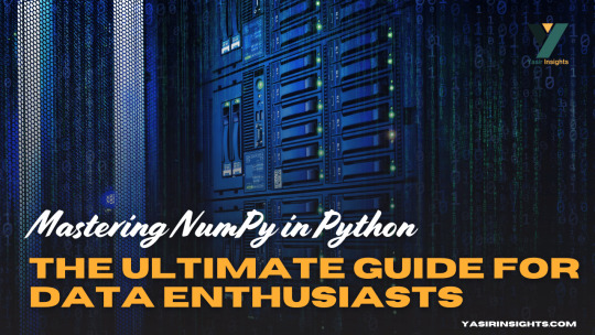
Imagine calculating the average of a million numbers using regular Python lists. You’d need to write multiple lines of code, deal with loops, and wait longer for the results. Now, what if you could do that in just one line? Enter NumPy in Python, the superhero of numerical computing in Python.
NumPy in Python (short for Numerical Python) is the core package that gives Python its scientific computing superpowers. It’s built for speed and efficiency, especially when working with arrays and matrices of numeric data. At its heart lies the ndarray—a powerful n-dimensional array object that’s much faster and more efficient than traditional Python lists.
What is NumPy in Python and Why It Matters
Why is NumPy a game-changer?
It allows operations on entire arrays without writing for-loops.
It’s written in C under the hood, so it’s lightning-fast.
It offers functionalities like Fourier transforms, linear algebra, random number generation, and so much more.
It’s compatible with nearly every scientific and data analysis library in Python like SciPy, Pandas, TensorFlow, and Matplotlib.
In short, if you’re doing data analysis, machine learning, or scientific research in Python, NumPy is your starting point.
The Evolution and Importance of NumPy in Python Ecosystem
Before NumPy in Python, Python had numeric libraries, but none were as comprehensive or fast. NumPy was developed to unify them all under one robust, extensible, and fast umbrella.
Created by Travis Oliphant in 2005, NumPy grew from an older package called Numeric. It soon became the de facto standard for numerical operations. Today, it’s the bedrock of almost every other data library in Python.
What makes it crucial?
Consistency: Most libraries convert input data into NumPy arrays for consistency.
Community: It has a huge support community, so bugs are resolved quickly and the documentation is rich.
Cross-platform: It runs on Windows, macOS, and Linux with zero change in syntax.
This tight integration across the Python data stack means that even if you’re working in Pandas or TensorFlow, you’re indirectly using NumPy under the hood.
Setting Up NumPy in Python
How to Install NumPy
Before using NumPy, you need to install it. The process is straightforward:
bash
pip install numpy
Alternatively, if you’re using a scientific Python distribution like Anaconda, NumPy comes pre-installed. You can update it using:
bash
conda update numpy
That’s it—just a few seconds, and you’re ready to start number-crunching!
Some environments (like Jupyter notebooks or Google Colab) already have NumPy installed, so you might not need to install it again.
Importing NumPy in Python and Checking Version
Once installed, you can import NumPy using the conventional alias:
python
import numpy as np
This alias, np, is universally recognized in the Python community. It keeps your code clean and concise.
To check your NumPy version:
python
print(np.__version__)
You’ll want to ensure that you’re using the latest version to access new functions, optimizations, and bug fixes.
If you’re just getting started, make it a habit to always import NumPy with np. It’s a small convention, but it speaks volumes about your code readability.
Understanding NumPy in Python Arrays
The ndarray Object – Core of NumPy
At the center of everything in NumPy lies the ndarray. This is a multidimensional, fixed-size container for elements of the same type.
Key characteristics:
Homogeneous Data: All elements are of the same data type (e.g., all integers or all floats).
Fast Operations: Built-in operations are vectorized and run at near-C speed.
Memory Efficiency: Arrays take up less space than lists.
You can create a simple array like this:
python
import numpy as np arr = np.array([1, 2, 3, 4])
Now arr is a NumPy array (ndarray), not just a Python list. The difference becomes clearer with larger data or when applying operations:
python
arr * 2 # [2 4 6 8]
It’s that easy. No loops. No complications.
You can think of an ndarray like an Excel sheet with superpowers—except it can be 1d, 2d, 3d, or even higher dimensions!
1-Dimensional Arrays – Basics and Use Cases
1d arrays are the simplest form—just a list of numbers. But don’t let the simplicity fool you. They’re incredibly powerful.
Creating a 1D array:
python
a = np.array([10, 20, 30, 40])
You can:
Multiply or divide each element by a number.
Add another array of the same size.
Apply mathematical functions like sine, logarithm, etc.
Example:
python
b = np.array([1, 2, 3, 4]) print(a + b) # Output: [11 22 33 44]
This concise syntax is possible because NumPy performs element-wise operations—automatically!
1d arrays are perfect for:
Mathematical modeling
Simple signal processing
Handling feature vectors in ML
Their real power emerges when used in batch operations. Whether you’re summing elements, calculating means, or applying a function to every value, 1D arrays keep your code clean and blazing-fast.
2-Dimensional Arrays – Matrices and Their Applications
2D arrays are like grids—rows and columns of data. They’re also the foundation of matrix operations in NumPy in Python.
You can create a 2D array like this:
python
arr_2d = np.array([[1, 2, 3], [4, 5, 6]])
Here’s what it looks like:
lua
[[1 2 3] [4 5 6]]
Each inner list becomes a row. This structure is ideal for:
Representing tables or datasets
Performing matrix operations like dot products
Image processing (since images are just 2D arrays of pixels)
Some key operations:
python
arr_2d.shape # (2, 3) — 2 rows, 3 columns arr_2d[0][1] # 2 — first row, second column arr_2d.T # Transpose: swaps rows and columns
You can also use slicing just like with 1d arrays:
python
arr_2d[:, 1] # All rows, second column => [2, 5] arr_2d[1, :] # Second row => [4, 5, 6]
2D arrays are extremely useful in:
Data science (e.g., CSVS loaded into 2D arrays)
Linear algebra (matrices)
Financial modelling and more
They’re like a spreadsheet on steroids—flexible, fast, and powerful.
3-Dimensional Arrays – Multi-Axis Data Representation
Now let’s add another layer. 3d arrays are like stacks of 2D arrays. You can think of them as arrays of matrices.
Here’s how you define one:
python
arr_3d = np.array([ [[1, 2], [3, 4]], [[5, 6], [7, 8]] ])
This array has:
2 matrices
Each matrix has 2 rows and 2 columns
Visualized as:
lua
[ [[1, 2], [3, 4]],[[5, 6], [7, 8]] ]
Accessing data:
python
arr_3d[0, 1, 1] # Output: 4 — first matrix, second row, second column
Use cases for 3D arrays:
Image processing (RGB images: height × width × color channels)
Time series data (time steps × variables × features)
Neural networks (3D tensors as input to models)
Just like with 2D arrays, NumPy’s indexing and slicing methods make it easy to manipulate and extract data from 3D arrays.
And the best part? You can still apply mathematical operations and functions just like you would with 1D or 2D arrays. It’s all uniform and intuitive.
Higher Dimensional Arrays – Going Beyond 3D
Why stop at 3D? NumPy in Python supports N-dimensional arrays (also called tensors). These are perfect when dealing with highly structured datasets, especially in advanced applications like:
Deep learning (4D/5D tensors for batching)
Scientific simulations
Medical imaging (like 3D scans over time)
Creating a 4D array:
python
arr_4d = np.random.rand(2, 3, 4, 5)
This gives you:
2 batches
Each with 3 matrices
Each matrix has 4 rows and 5 columns
That’s a lot of data—but NumPy handles it effortlessly. You can:
Access any level with intuitive slicing
Apply functions across axes
Reshape as needed using .reshape()
Use arr.ndim to check how many dimensions you’re dealing with. Combine that with .shape, and you’ll always know your array’s layout.
Higher-dimensional arrays might seem intimidating, but NumPy in Python makes them manageable. Once you get used to 2D and 3D, scaling up becomes natural.
NumPy in Python Array Creation Techniques
Creating Arrays Using Python Lists
The simplest way to make a NumPy array is by converting a regular Python list:
python
a = np.array([1, 2, 3])
Or a list of lists for 2D arrays:
python
b = np.array([[1, 2], [3, 4]])
You can also specify the data type explicitly:
python
np.array([1, 2, 3], dtype=float)
This gives you a float array [1.0, 2.0, 3.0]. You can even convert mixed-type lists, but NumPy will automatically cast to the most general type to avoid data loss.
Pro Tip: Always use lists of equal lengths when creating 2D+ arrays. Otherwise, NumPy will make a 1D array of “objects,” which ruins performance and vectorization.
Array Creation with Built-in Functions (arange, linspace, zeros, ones, etc.)
NumPy comes with handy functions to quickly create arrays without writing out all the elements.
Here are the most useful ones:
np.arange(start, stop, step): Like range() but returns an array.
np.linspace(start, stop, num): Evenly spaced numbers between two values.
np.zeros(shape): Array filled with zeros.
np.ones(shape): Array filled with ones.
np.eye(N): Identity matrix.
These functions help you prototype, test, and create arrays faster. They also avoid manual errors and ensure your arrays are initialized correctly.
Random Array Generation with random Module
Need to simulate data? NumPy’s random module is your best friend.
python
np.random.rand(2, 3) # Uniform distribution np.random.randn(2, 3) # Normal distribution np.random.randint(0, 10, (2, 3)) # Random integers
You can also:
Shuffle arrays
Choose random elements
Set seeds for reproducibility (np.random.seed(42))
This is especially useful in:
Machine learning (generating datasets)
Monte Carlo simulations
Statistical experiments.
Reshaping, Flattening, and Transposing Arrays
Reshaping is one of NumPy’s most powerful features. It lets you reorganize the shape of an array without changing its data. This is critical when preparing data for machine learning models or mathematical operations.
Here’s how to reshape:
python
a = np.array([1, 2, 3, 4, 5, 6]) b = a.reshape(2, 3) # Now it's 2 rows and 3 columns
Reshaped arrays can be converted back using .flatten():
python
flat = b.flatten() # [1 2 3 4 5 6]
There’s also .ravel()—similar to .flatten() but returns a view if possible (faster and more memory-efficient).
Transposing is another vital transformation:
python
matrix = np.array([[1, 2], [3, 4]]) matrix.T # Output: # [[1 3] # [2 4]]
Transpose is especially useful in linear algebra, machine learning (swapping features with samples), and when matching shapes for operations like matrix multiplication.
Use .reshape(-1, 1) to convert arrays into columns, and .reshape(1, -1) to make them rows. This flexibility gives you total control over the structure of your data.
Array Slicing and Indexing Tricks
You can access parts of an array using slicing, which works similarly to Python lists but more powerful in NumPy in Python.
Basic slicing:
python
arr = np.array([10, 20, 30, 40, 50]) arr[1:4] # [20 30 40]
2D slicing:
python
mat = np.array([[1, 2, 3], [4, 5, 6], [7, 8, 9]]) mat[0:2, 1:] # Rows 0-1, columns 1-2 => [[2 3], [5 6]]
Advanced indexing includes:
Boolean indexing:
python
arr[arr > 30] # Elements greater than 30
Fancy indexing:
python
arr[[0, 2, 4]] # Elements at indices 0, 2, 4
Modifying values using slices:
python
arr[1:4] = 99 # Replace elements at indices 1 to 3
Slices return views, not copies. So if you modify a slice, the original array is affected—unless you use .copy().
These slicing tricks make data wrangling fast and efficient, letting you filter and extract patterns in seconds.
Broadcasting and Vectorized Operations
Broadcasting is what makes NumPy in Python shine. It allows operations on arrays of different shapes and sizes without writing explicit loops.
Let’s say you have a 1D array:
python
a = np.array([1, 2, 3])
And a scalar:
python
b = 10
You can just write:
python
c = a + b # [11, 12, 13]
That’s broadcasting in action. It also works for arrays with mismatched shapes as long as they are compatible:
python
a = np.array([[1], [2], [3]]) # Shape (3,1) b = np.array([4, 5, 6]) # Shape (3,)a + b
This adds each element to each element b, creating a full matrix.
Why is this useful?
It avoids for-loops, making your code cleaner and faster
It matches standard mathematical notation
It enables writing expressive one-liners
Vectorization uses broadcasting behind the scenes to perform operations efficiently:
python
a * b # Element-wise multiplication np.sqrt(a) # Square root of each element np.exp(a) # Exponential of each element
These tricks make NumPy in Python code shorter, faster, and far more readable.
Mathematical and Statistical Operations
NumPy offers a rich suite of math functions out of the box.
Basic math:
python
np.add(a, b) np.subtract(a, b) np.multiply(a, b) np.divide(a, b)
Aggregate functions:
python
np.sum(a) np.mean(a) np.std(a) np.var(a) np.min(a) np.max(a)
Axis-based operations:
python
arr_2d = np.array([[1, 2, 3], [4, 5, 6]]) np.sum(arr_2d, axis=0) # Sum columns: [5 7 9] np.sum(arr_2d, axis=1) # Sum rows: [6 15]
Linear algebra operations:
python
np.dot(a, b) # Dot product np.linalg.inv(mat) # Matrix inverse np.linalg.det(mat) # Determinant np.linalg.eig(mat) # Eigenvalues
Statistical functions:
python
np.percentile(a, 75) np.median(a) np.corrcoef(a, b)
Trigonometric operations:
python
np.sin(a) np.cos(a) np.tan(a)
These functions let you crunch numbers, analyze trends, and model complex systems in just a few lines.
NumPy in Python I/O – Saving and Loading Arrays
Data persistence is key. NumPy in Python lets you save and load arrays easily.
Saving arrays:
python
np.save('my_array.npy', a) # Saves in binary format
Loading arrays:
python
b = np.load('my_array.npy')
Saving multiple arrays:
python
np.savez('data.npz', a=a, b=b)
Loading multiple arrays:
python
data = np.load('data.npz') print(data['a']) # Access saved 'a' array
Text file operations:
python
np.savetxt('data.txt', a, delimiter=',') b = np.loadtxt('data.txt', delimiter=',')
Tips:
Use .npy or .npz formats for efficiency
Use .txt or .csv for interoperability
Always check array shapes after loading
These functions allow seamless transition between computations and storage, critical for real-world data workflows.
Masking, Filtering, and Boolean Indexing
NumPy in Python allows you to manipulate arrays with masks—a powerful way to filter and operate on elements that meet certain conditions.
Here’s how masking works:
python
arr = np.array([10, 20, 30, 40, 50]) mask = arr > 25
Now mask is a Boolean array:
graphql
[False False True True True]
You can use this mask to extract elements:
python
filtered = arr[mask] # [30 40 50]
Or do operations:
python
arr[mask] = 0 # Set all elements >25 to 0
Boolean indexing lets you do conditional replacements:
python
arr[arr < 20] = -1 # Replace all values <20
This technique is extremely useful in:
Cleaning data
Extracting subsets
Performing conditional math
It’s like SQL WHERE clauses but for arrays—and lightning-fast.
Sorting, Searching, and Counting Elements
Sorting arrays is straightforward:
python
arr = np.array([10, 5, 8, 2]) np.sort(arr) # [2 5 8 10]
If you want to know the index order:
python
np.argsort(arr) # [3 1 2 0]
Finding values:
python
np.where(arr > 5) # Indices of elements >5
Counting elements:
python
np.count_nonzero(arr > 5) # How many elements >5
You can also use np.unique() to find unique values and their counts:
python
np.unique(arr, return_counts=True)
Need to check if any or all elements meet a condition?
python
np.any(arr > 5) # True if any >5 np.all(arr > 5) # True if all >5
These operations are essential when analyzing and transforming datasets.
Copy vs View in NumPy in Python – Avoiding Pitfalls
Understanding the difference between a copy and a view can save you hours of debugging.
By default, NumPy tries to return views to save memory. But modifying a view also changes the original array.
Example of a view:
python
a = np.array([1, 2, 3]) b = a[1:] b[0] = 99 print(a) # [1 99 3] — original changed!
If you want a separate copy:
python
b = a[1:].copy()
Now b is independent.
How to check if two arrays share memory?
python
np.may_share_memory(a, b)
When working with large datasets, always ask yourself—is this a view or a copy? Misunderstanding this can lead to subtle bugs.
Useful NumPy Tips and Tricks
Let’s round up with some power-user tips:
Memory efficiency: Use dtype to optimize storage. For example, use np.int8 instead of the default int64 for small integers.
Chaining: Avoid chaining operations that create temporary arrays. Instead, use in-place ops like arr += 1.
Use .astype() For type conversion:
Suppress scientific notation:
Timing your code:
Broadcast tricks:
These make your code faster, cleaner, and more readable.
Integration with Other Libraries (Pandas, SciPy, Matplotlib)
NumPy plays well with others. Most scientific libraries in Python depend on it:
Pandas
Under the hood, pandas.DataFrame uses NumPy arrays.
You can extract or convert between the two seamlessly:
Matplotlib
Visualizations often start with NumPy arrays:
SciPy
Built on top of NumPy
Adds advanced functionality like optimization, integration, statistics, etc.
Together, these tools form the backbone of the Python data ecosystem.
Conclusion
NumPy is more than just a library—it’s the backbone of scientific computing in Python. Whether you’re a data analyst, machine learning engineer, or scientist, mastering NumPy gives you a massive edge.
Its power lies in its speed, simplicity, and flexibility:
Create arrays of any dimension
Perform operations in vectorized form
Slice, filter, and reshape data in milliseconds
Integrate easily with tools like Pandas, Matplotlib, and SciPy
Learning NumPy isn’t optional—it’s essential. And once you understand how to harness its features, the rest of the Python data stack falls into place like magic.
So fire up that Jupyter notebook, start experimenting, and make NumPy your new best friend.
FAQs
1. What’s the difference between a NumPy array and a Python list? A NumPy array is faster, uses less memory, supports vectorized operations, and requires all elements to be of the same type. Python lists are more flexible but slower for numerical computations.
2. Can I use NumPy for real-time applications? Yes! NumPy is incredibly fast and can be used in real-time data analysis pipelines, especially when combined with optimized libraries like Numba or Cython.
3. What’s the best way to install NumPy? Use pip or conda. For pip: pip install numpy, and for conda: conda install numpy.
4. How do I convert a Pandas DataFrame to a NumPy array? Just use .values or .to_numpy():
python
array = df.to_numpy()
5. Can NumPy handle missing values? Not directly like Pandas, but you can use np.nan and functions like np.isnan() and np.nanmean() to handle NaNs.
0 notes
Text
OneAPI Math Kernel Library (oneMKL): Intel MKL’s Successor

The upgraded and enlarged Intel oneAPI Math Kernel Library supports numerical processing not only on CPUs but also on GPUs, FPGAs, and other accelerators that are now standard components of heterogeneous computing environments.
In order to assist you decide if upgrading from traditional Intel MKL is the better option for you, this blog will provide you with a brief summary of the maths library.
Why just oneMKL?
The vast array of mathematical functions in oneMKL can be used for a wide range of tasks, from straightforward ones like linear algebra and equation solving to more intricate ones like data fitting and summary statistics.
Several scientific computing functions, including vector math, fast Fourier transforms (FFT), random number generation (RNG), dense and sparse Basic Linear Algebra Subprograms (BLAS), Linear Algebra Package (LAPLACK), and vector math, can all be applied using it as a common medium while adhering to uniform API conventions. Together with GPU offload and SYCL support, all of these are offered in C and Fortran interfaces.
Additionally, when used with Intel Distribution for Python, oneAPI Math Kernel Library speeds up Python computations (NumPy and SciPy).
Intel MKL Advanced with oneMKL
A refined variant of the standard Intel MKL is called oneMKL. What sets it apart from its predecessor is its improved support for SYCL and GPU offload. Allow me to quickly go over these two distinctions.
GPU Offload Support for oneMKL
GPU offloading for SYCL and OpenMP computations is supported by oneMKL. With its main functionalities configured natively for Intel GPU offload, it may thus take use of parallel-execution kernels of GPU architectures.
oneMKL adheres to the General Purpose GPU (GPGPU) offload concept that is included in the Intel Graphics Compute Runtime for OpenCL Driver and oneAPI Level Zero. The fundamental execution mechanism is as follows: the host CPU is coupled to one or more compute devices, each of which has several GPU Compute Engines (CE).
SYCL API for oneMKL
OneMKL’s SYCL API component is a part of oneAPI, an open, standards-based, multi-architecture, unified framework that spans industries. (Khronos Group’s SYCL integrates the SYCL specification with language extensions created through an open community approach.) Therefore, its advantages can be reaped on a variety of computing devices, including FPGAs, CPUs, GPUs, and other accelerators. The SYCL API’s functionality has been divided into a number of domains, each with a corresponding code sample available at the oneAPI GitHub repository and its own namespace.
OneMKL Assistance for the Most Recent Hardware
On cutting-edge architectures and upcoming hardware generations, you can benefit from oneMKL functionality and optimizations. Some examples of how oneMKL enables you to fully utilize the capabilities of your hardware setup are as follows:
It supports the 4th generation Intel Xeon Scalable Processors’ float16 data type via Intel Advanced Vector Extensions 512 (Intel AVX-512) and optimised bfloat16 and int8 data types via Intel Advanced Matrix Extensions (Intel AMX).
It offers matrix multiply optimisations on the upcoming generation of CPUs and GPUs, including Single Precision General Matrix Multiplication (SGEMM), Double Precision General Matrix Multiplication (DGEMM), RNG functions, and much more.
For a number of features and optimisations on the Intel Data Centre GPU Max Series, it supports Intel Xe Matrix Extensions (Intel XMX).
For memory-bound dense and sparse linear algebra, vector math, FFT, spline computations, and various other scientific computations, it makes use of the hardware capabilities of Intel Xeon processors and Intel Data Centre GPUs.
Additional Terms and Context
The brief explanation of terminology provided below could also help you understand oneMKL and how it fits into the heterogeneous-compute ecosystem.
The C++ with SYCL interfaces for performance math library functions are defined in the oneAPI Specification for oneMKL. The oneMKL specification has the potential to change more quickly and often than its implementations.
The specification is implemented in an open-source manner by the oneAPI Math Kernel Library (oneMKL) Interfaces project. With this project, we hope to show that the SYCL interfaces described in the oneMKL specification may be implemented for any target hardware and math library.
The intention is to gradually expand the implementation, even though the one offered here might not be the complete implementation of the specification. We welcome community participation in this project, as well as assistance in expanding support to more math libraries and a variety of hardware targets.
With C++ and SYCL interfaces, as well as comparable capabilities with C and Fortran interfaces, oneMKL is the Intel product implementation of the specification. For Intel CPU and Intel GPU hardware, it is extremely optimized.
Next up, what?
Launch oneMKL now to begin speeding up your numerical calculations like never before! Leverage oneMKL’s powerful features to expedite math processing operations and improve application performance while reducing development time for both current and future Intel platforms.
Keep in mind that oneMKL is rapidly evolving even while you utilize the present features and optimizations! In an effort to keep up with the latest Intel technology, we continuously implement new optimizations and support for sophisticated math functions.
They also invite you to explore the AI, HPC, and Rendering capabilities available in Intel’s software portfolio that is driven by oneAPI.
Read more on govindhtech.com
#FPGAs#CPU#GPU#inteloneapi#onemkl#python#IntelGraphics#IntelTechnology#mathkernellibrary#API#news#technews#technology#technologynews#technologytrends#govindhtech
0 notes
Text
"Top Software Training Courses"
In the rapidly evolving landscape of technology, staying updated with the latest skills and knowledge is crucial for professionals in the software industry. Quality software training courses can provide individuals with the expertise needed to excel in their careers and contribute meaningfully to their organizations. Here are some of the top software training courses that cover a wide range of technologies and skill sets.
1. "The Complete Web Developer Course 2.0" by Rob Percival
This comprehensive course covers web development from front-end to back-end, including HTML, CSS, JavaScript, Node.js, and MongoDB. With hands-on projects and practical exercises, students gain practical experience in building responsive websites and web applications.
2. "Machine Learning A-Z™: Hands-On Python & R In Data Science" by Kirill Eremenko and Hadelin de Ponteves
Ideal for aspiring data scientists and machine learning enthusiasts, this course covers a wide range of machine learning algorithms and techniques using Python and R. Students learn how to apply machine learning to real-world problems and build predictive models.
3. "iOS 13 & Swift 5 - The Complete iOS App Development Bootcamp" by Dr. Angela Yu
Designed for beginners and intermediate developers, this bootcamp covers iOS app development using Swift 5 and Xcode 11. Students learn how to build full-fledged iOS apps, including user interfaces, data storage, networking, and app deployment.
4. "The Complete JavaScript Course 2021: From Zero to Expert!" by Jonas Schmedtmann
This comprehensive course covers JavaScript programming from beginner to advanced levels. Students learn essential JavaScript concepts, such as variables, functions, arrays, and objects, as well as advanced topics like asynchronous JavaScript and modern ES6+ features.
5. "Python for Data Science and Machine Learning Bootcamp" by Jose Portilla
Ideal for individuals interested in data science and machine learning, this bootcamp covers Python programming, data analysis, machine learning, and data visualization using libraries such as NumPy, Pandas, Matplotlib, Seaborn, and Scikit-learn.
6. "React - The Complete Guide (incl Hooks, React Router, Redux)" by Maximilian Schwarzmüller
This comprehensive course covers React.js, a popular JavaScript library for building user interfaces. Students learn React fundamentals, including components, props, state, and hooks, as well as advanced topics like React Router and Redux for state management.
7. "Docker Mastery: with Kubernetes +Swarm from a Docker Captain" by Bret Fisher
Ideal for DevOps engineers and system administrators, this course covers Docker and Kubernetes, two popular containerization technologies used for deploying and managing applications. Students learn how to build, deploy, and scale containerized applications using Docker and Kubernetes.
Conclusion
These top software training courses cover a wide range of technologies and skill sets, including web development, machine learning, iOS app development, JavaScript, Python, React.js, Docker, and Kubernetes. Whether you're a beginner looking to get started in a new field or an experienced developer seeking to expand your skill set, these courses offer valuable resources and practical insights to help you succeed in the software industry. By investing time and effort in learning from these courses, you'll be well-equipped to tackle the challenges and opportunities in the ever-evolving world of technology.
Read more
#software#training#information technology#software training institute#it training institute#online courses#it training courses
0 notes
Text
Large Language Models with Scikit-learn: A Comprehensive Guide to Scikit-LLM
New Post has been published on https://thedigitalinsider.com/large-language-models-with-scikit-learn-a-comprehensive-guide-to-scikit-llm/
Large Language Models with Scikit-learn: A Comprehensive Guide to Scikit-LLM
By integrating the sophisticated language processing capabilities of models like ChatGPT with the versatile and widely-used Scikit-learn framework, Scikit-LLM offers an unmatched arsenal for delving into the complexities of textual data.
Scikit-LLM, accessible on its official GitHub repository, represents a fusion of – the advanced AI of Large Language Models (LLMs) like OpenAI’s GPT-3.5 and the user-friendly environment of Scikit-learn. This Python package, specially designed for text analysis, makes advanced natural language processing accessible and efficient.
Why Scikit-LLM?
For those well-versed in Scikit-learn’s landscape, Scikit-LLM feels like a natural progression. It maintains the familiar API, allowing users to utilize functions like .fit(), .fit_transform(), and .predict(). Its ability to integrate estimators into a Sklearn pipeline exemplifies its flexibility, making it a boon for those looking to enhance their machine learning projects with state-of-the-art language understanding.
In this article, we explore Scikit-LLM, from its installation to its practical application in various text analysis tasks. You’ll learn how to create both supervised and zero-shot text classifiers and delve into advanced features like text vectorization and classification.
Scikit-learn: The Cornerstone of Machine Learning
Before diving into Scikit-LLM, let’s touch upon its foundation – Scikit-learn. A household name in machine learning, Scikit-learn is celebrated for its comprehensive algorithmic suite, simplicity, and user-friendliness. Covering a spectrum of tasks from regression to clustering, Scikit-learn is the go-to tool for many data scientists.
Built on the bedrock of Python’s scientific libraries (NumPy, SciPy, and Matplotlib), Scikit-learn stands out for its integration with Python’s scientific stack and its efficiency with NumPy arrays and SciPy sparse matrices.
At its core, Scikit-learn is about uniformity and ease of use. Regardless of the algorithm you choose, the steps remain consistent – import the class, use the ‘fit’ method with your data, and apply ‘predict’ or ‘transform’ to utilize the model. This simplicity reduces the learning curve, making it an ideal starting point for those new to machine learning.
Setting Up the Environment
Before diving into the specifics, it’s crucial to set up the working environment. For this article, Google Colab will be the platform of choice, providing an accessible and powerful environment for running Python code.
Installation
%%capture !pip install scikit-llm watermark %load_ext watermark %watermark -a "your-username" -vmp scikit-llm
Obtaining and Configuring API Keys
Scikit-LLM requires an OpenAI API key for accessing the underlying language models.
from skllm.config import SKLLMConfig OPENAI_API_KEY = "sk-****" OPENAI_ORG_ID = "org-****" SKLLMConfig.set_openai_key(OPENAI_API_KEY) SKLLMConfig.set_openai_org(OPENAI_ORG_ID)
Zero-Shot GPTClassifier
The ZeroShotGPTClassifier is a remarkable feature of Scikit-LLM that leverages ChatGPT’s ability to classify text based on descriptive labels, without the need for traditional model training.
Importing Libraries and Dataset
from skllm import ZeroShotGPTClassifier from skllm.datasets import get_classification_dataset X, y = get_classification_dataset()
Preparing the Data
Splitting the data into training and testing subsets:
def training_data(data): return data[:8] + data[10:18] + data[20:28] def testing_data(data): return data[8:10] + data[18:20] + data[28:30] X_train, y_train = training_data(X), training_data(y) X_test, y_test = testing_data(X), testing_data(y)
Model Training and Prediction
Defining and training the ZeroShotGPTClassifier:
clf = ZeroShotGPTClassifier(openai_model="gpt-3.5-turbo") clf.fit(X_train, y_train) predicted_labels = clf.predict(X_test)
Evaluation
Evaluating the model’s performance:
from sklearn.metrics import accuracy_score print(f"Accuracy: accuracy_score(y_test, predicted_labels):.2f")
Text Summarization with Scikit-LLM
Text summarization is a critical feature in the realm of NLP, and Scikit-LLM harnesses GPT’s prowess in this domain through its GPTSummarizer module. This feature stands out for its adaptability, allowing it to be used both as a standalone tool for generating summaries and as a preprocessing step in broader workflows.
Applications of GPTSummarizer:
Standalone Summarization: The GPTSummarizer can independently create concise summaries from lengthy documents, which is invaluable for quick content analysis or extracting key information from large volumes of text.
Preprocessing for Other Operations: In workflows that involve multiple stages of text analysis, the GPTSummarizer can be used to condense text data. This reduces the computational load and simplifies subsequent analysis steps without losing essential information.
Implementing Text Summarization:
The implementation process for text summarization in Scikit-LLM involves:
Importing GPTSummarizer and the relevant dataset.
Creating an instance of GPTSummarizer with specified parameters like max_words to control summary length.
Applying the fit_transform method to generate summaries.
It’s important to note that the max_words parameter serves as a guideline rather than a strict limit, ensuring summaries maintain coherence and relevance, even if they slightly exceed the specified word count.
Broader Implications of Scikit-LLM
Scikit-LLM’s range of features, including text classification, summarization, vectorization, translation, and its adaptability in handling unlabeled data, makes it a comprehensive tool for diverse text analysis tasks. This flexibility and ease of use cater to both novices and experienced practitioners in the field of AI and machine learning.
Potential Applications:
Customer Feedback Analysis: Classifying customer feedback into categories like positive, negative, or neutral, which can inform customer service improvements or product development strategies.
News Article Classification: Sorting news articles into various topics for personalized news feeds or trend analysis.
Language Translation: Translating documents for multinational operations or personal use.
Document Summarization: Quickly grasping the essence of lengthy documents or creating shorter versions for publication.
Advantages of Scikit-LLM:
Accuracy: Proven effectiveness in tasks like zero-shot text classification and summarization.
Speed: Suitable for real-time processing tasks due to its efficiency.
Scalability: Capable of handling large volumes of text, making it ideal for big data applications.
Conclusion: Embracing Scikit-LLM for Advanced Text Analysis
In summary, Scikit-LLM stands as a powerful, versatile, and user-friendly tool in the realm of text analysis. Its ability to combine Large Language Models with traditional machine learning workflows, coupled with its open-source nature, makes it a valuable asset for researchers, developers, and businesses alike. Whether it’s refining customer service, analyzing news trends, facilitating multilingual communication, or distilling essential information from extensive documents, Scikit-LLM offers a robust solution.
#ai#algorithm#Analysis#API#applications#Arrays#Art#Article#Articles#Artificial General Intelligence#Big Data#Capture#chatGPT#code#CoLab#communication#comprehensive#content#customer service#data#datasets#developers#development#diving#efficiency#Environment#Experienced#Features#Foundation#framework
0 notes
Text
Python Numpy Tutorials
#python numpy tutorials#numpy zeros array#what is zero array in python#how to create a zero numpy array#how to create arrays in python#numpy tutorials#numpy zeros function#how to create an array of zeros#python ones array#python zeros and ones arrays#numpy tutorials for beginners#zeros arrays#zero array in python#zeros arrays in numpy#how to use zeros array python numpy#difference between zeros and ones arrays in python numpy#zeros one two three dimen array#shiva
0 notes
Text
Master NumPy Library for Data Analysis in Python in 10 Minutes
Learn and Become a Master of one of the most used Python tools for Data Analysis.

Introduction:-
NumPy is a python library used for working with arrays.It also has functions for working in domain of linear algebra, fourier transform, and matrices.It is an open source project and you can use it freely. NumPy stands for Numerical Python.
NumPy — Ndarray Object
The most important object defined in NumPy is an N-dimensional array type called ndarray. It describes the collection of items of the same type. Items in the collection can be accessed using a zero-based index.Every item in an ndarray takes the same size of block in the memory.
Each element in ndarray is an object of data-type object (called dtype).Any item extracted from ndarray object (by slicing) is represented by a Python object of one of array scalar types.
The following diagram shows a relationship between ndarray, data type object (dtype) and array scalar type −
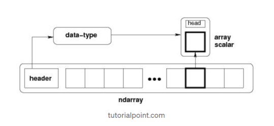
It creates an ndarray from any object exposing array interface, or from any method that returns an array.
numpy.array(object, dtype = None, copy = True, order = None, subok = False, ndmin = 0)
The above constructor takes the following parameters −
Object :- Any object exposing the array interface method returns an array, or any (nested) sequence.
Dtype : — Desired data type of array, optional.
Copy :- Optional. By default (true), the object is copied.
Order :- C (row major) or F (column major) or A (any) (default).
Subok :- By default, returned array forced to be a base class array. If true, sub-classes passed through.
ndmin :- Specifies minimum dimensions of resultant array.
Operations on Numpy Array
In this blog, we’ll walk through using NumPy to analyze data on wine quality. The data contains information on various attributes of wines, such as pH and fixed acidity, along with a quality score between 0 and 10 for each wine. The quality score is the average of at least 3 human taste testers. As we learn how to work with NumPy, we’ll try to figure out more about the perceived quality of wine.
The data was downloaded from the winequality-red.csv, and is available here. file, which we’ll be using throughout this tutorial:
Lists Of Lists for CSV Data
Before using NumPy, we’ll first try to work with the data using Python and the csv package. We can read in the file using the csv.reader object, which will allow us to read in and split up all the content from the ssv file.
In the below code, we:
Import the csv library.
Open the winequality-red.csv file.
With the file open, create a new csv.reader object.
Pass in the keyword argument delimiter=";" to make sure that the records are split up on the semicolon character instead of the default comma character.
Call the list type to get all the rows from the file.
Assign the result to wines.
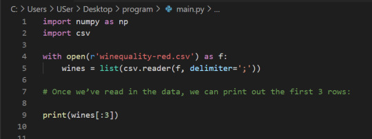
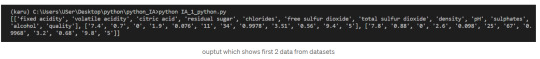
We can check the number of rows and columns in our data using the shape property of NumPy arrays:
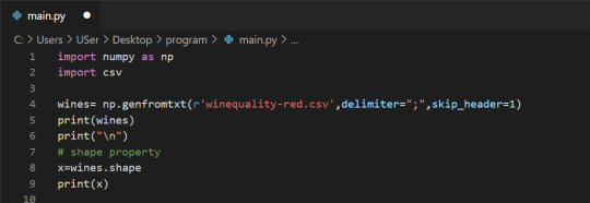
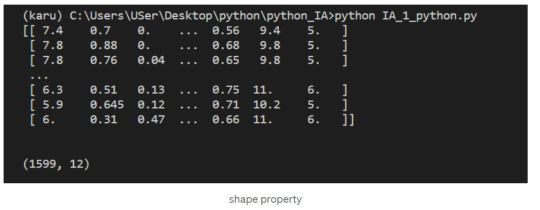
Indexing NumPy Arrays
Let’s select the element at row 3 and column 4. In the below code, we pass in the index 2 as the row index, and the index 3 as the column index. This retrieves the value from the fourth column of the third row:
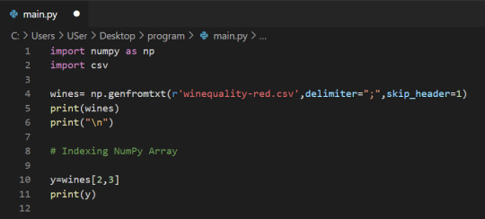
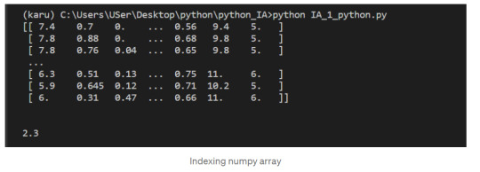
1-Dimensional NumPy Arrays
So far, we’ve worked with 2-dimensional arrays, such as wines. However, NumPy is a package for working with multidimensional arrays. One of the most common types of multidimensional arrays is the 1-dimensional array, or vector.
1.Just like a list of lists is analogous to a 2-dimensional array, a single list is analogous to a 1-dimensional array. If we slice wines and only retrieve the third row, we get a 1-dimensional array:
2. We can retrieve individual elements from third_wine using a single index. The below code will display the second item in third_wine:
3. Most NumPy functions that we’ve worked with, such as numpy.random.rand, can be used with multidimensional arrays. Here’s how we’d use numpy.random.rand to generate a random vector:
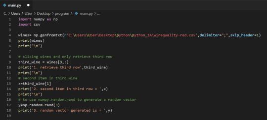
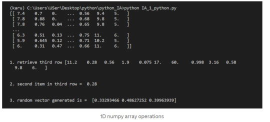
After successfully reading our dataset and learning about List, Indexing, & 1D array in NumPy we can start performing the operation on it.
The first element of each row is the fixed acidity, the second is the volatile ,acidity, and so on. We can find the average quality of the wines. The below code will:
Extract the last element from each row after the header row.
Convert each extracted element to a float.
Assign all the extracted elements to the list qualities.
Divide the sum of all the elements in qualities by the total number of elements in qualities to the get the mean.
NumPy Array Methods
In addition to the common mathematical operations, NumPy also has several methods that you can use for more complex calculations on arrays. An example of this is the numpy.ndarray.sum method. This finds the sum of all the elements in an array by default:
2. Sum of alcohol content in all sample red wines
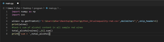
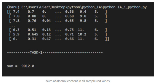
NumPy Array Comparisons
We get a Boolean array that tells us which of the wines have a quality rating greater than 5. We can do something similar with the other operators. For instance, we can see if any wines have a quality rating equal to 10:
3. select wines having pH content > 5
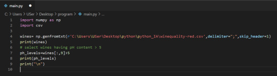
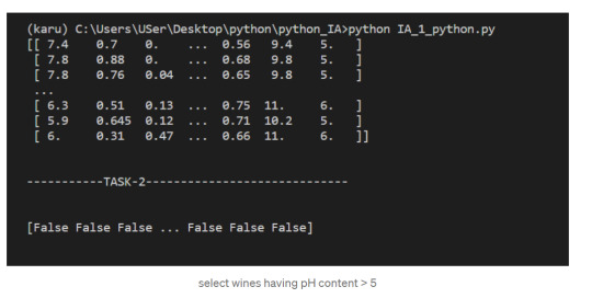
Subsetting
We select only the rows where high_Quality contains a True value, and all of the columns. This subsetting makes it simple to filter arrays for certain criteria. For example, we can look for wines with a lot of alcohol and high quality. In order to specify multiple conditions, we have to place each condition in parentheses, and separate conditions with an ampersand (&):
4. Select only wines where sulphates >10 and alcohol >7
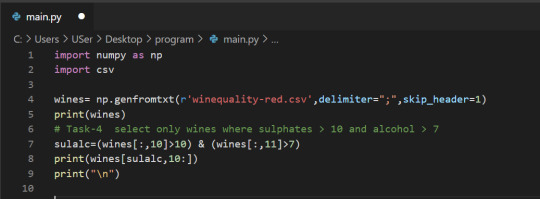
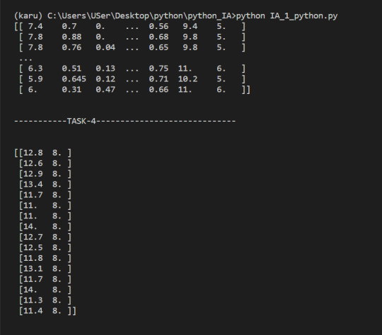
5. select wine having pH greater than mean pH
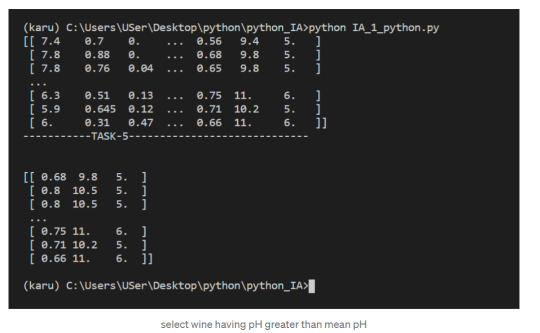
We have seen what NumPy is, and some of its most basic uses. In the following posts we will see more complex functionalities and dig deeper into the workings of this fantastic library!
To check it out follow me on tumblr, and stay tuned!
That is all, I hope you liked the post. Feel Free to follow me on tumblr
Also, you can take a look at my other posts on Data Science and Machine Learning here. Have a good read!
1 note
·
View note
Text
Trying out AWS SageMaker Studio for a simple machine learning task
Overview
Let’s look at how to accomplish a simple machine learning task on
AWS SageMaker
We'll take a movie ratings dataset comprising of user ratings for different movies and the movie metadata. Based on these existing user ratings of different movies, we'll try to predict what the user's rating would be for a movie that they haven't rated yet.
The following two documents are the primary references used in creating this doc - so feel free to refer to them in case there are any issues.
[1] Build, Train, and Deploy a Machine Learning Model (https://aws.amazon.com/getting-started/hands-on/build-train-deploy-machine-learning-model-sagemaker/) [2] Machine Learning Project – Data Science Movie Recommendation System Project in R (https://data-flair.training/blogs/data-science-r-movie-recommendation/)
We'd be using the MovieLens data from GroupLens Research.
[3] MovieLens | GroupLens (https://grouplens.org/datasets/movielens/)
Steps
Log into the AWS console and select Amazon SageMaker from the services to be redirected to the SageMaker Dashboard.
Select Amazon SageMaker Studio from the navigation bar on the left and select quick start to start a new instance of Amazon SageMaker Studio. Consider leaving the default name as is, select "Create a new role" in execution role and specify the S3 buckets you'd be using (Leaving these defaults should be okay as well) and click "Create Role". Once the execution role has been created, click on “Submit” - this will create a new Amazon SageMaker instance.
Once the Amazon SageMaker Studio instance is created, click on Open Studio link to launch the Amazon SageMaker Studio IDE.
Create a new Jupyter notebook using the Data Science as the Kernel and the latest python (Python 3) notebook.
Import the python libraries we'd be using in this task - boto3 is the python library which is used for making AWS requests, sagemaker is the sagemaker library and urllib.request is the library to make url requests such as HTTP GET etc to download csv files stored on S3 and elsewhere. numpy is a scientific computing python library and pandas is a python data analysis library. After writing the following code in the Jupyter notebook cell, look for a play button in the controls bar on top - click it should run the currently active cell and execute its code.
import boto3, sagemaker, urllib.request from sagemaker import get_execution_role import numpy as np import pandas as pd from sagemaker.predictor import csv_serializer
Once the imports have been completed, lets add some standard code to create execution role, define region settings and initialize boto for the region and xgboost
# Define IAM role role = get_execution_role() prefix = 'sagemaker/movielens' containers = {'us-west-2': '433757028032.dkr.ecr.us-west-2.amazonaws.com/xgboost:latest', 'us-east-1': '811284229777.dkr.ecr.us-east-1.amazonaws.com/xgboost:latest', 'us-east-2': '825641698319.dkr.ecr.us-east-2.amazonaws.com/xgboost:latest', 'eu-west-1': '685385470294.dkr.ecr.eu-west-1.amazonaws.com/xgboost:latest'} # each region has its XGBoost container my_region = boto3.session.Session().region_name # set the region of the instance print("Success - the MySageMakerInstance is in the " + my_region + " region. You will use the " + containers[my_region] + " container for your SageMaker endpoint.")
Create an S3 bucket that will contain our dataset files as well as training, test data, the computed machine learning models and the results.
bucket_name = '<BUCKET_NAME_HERE>' s3 = boto3.resource('s3') try: if my_region == 'us-east-1': s3.create_bucket(Bucket=bucket_name) else: s3.create_bucket(Bucket=bucket_name, CreateBucketConfiguration={ 'LocationConstraint': my_region }) print('S3 bucket created successfully') except Exception as e: print('S3 error: ',e)
Once the bucket has been created, upload the movie lens data files to the bucket by using the S3 console UI. You'll need to download the zip from https://grouplens.org/datasets/movielens/, extract it on the local machine and then upload the extracted files on S3. We used the Small dataset which has 100,000 ratings applied to 9,000 movies by 600 users. Be sure to read the MovieLens README file to make sure you understand the conditions on the data usage.
After the files have been uploaded, add the following code to the notebook to download the csv files and convert them to pandas data format
try: urllib.request.urlretrieve ("https://{}.s3.{}.amazonaws.com/ratings.csv".format(bucket_name, my_region), "ratings.csv") print('Success: downloaded ratings.csv.') except Exception as e: print('Data load error: ',e) try: urllib.request.urlretrieve ("https://{}.s3.{}.amazonaws.com/movies.csv".format(bucket_name, my_region), "movies.csv") print('Success: downloaded ratings.csv.') except Exception as e: print('Data load error: ',e)
try: model_data = pd.read_csv('./ratings.csv') print('Success: Data loaded into dataframe.') except Exception as e: print('Data load error: ',e) try: movie_data = pd.read_csv('./movies.csv') print('Success: Data loaded into dataframe.') except Exception as e: print('Data load error: ',e)
Now we create training and test datasets from the ratings data by splitting 70-30% the data randomly
train_data, test_data = np.split(model_data.sample(frac=1, random_state=1729), [int(0.7 * len(model_data))]) print(train_data.shape, test_data.shape) print(train_data.info, test_data.info)
We will need to normalize the training and test datasets to include boolean genre membership columns for each genre. To do this, we first process the movie dataset to create a movie to list of its genres map. Once the map has been created, we iterate the ratings data and update each row with the boolean genre membership columns. The following code creates the movie genre maps
movie_id_genre_map=dict() for movie_row in movie_data.itertuples(): # print (movie_row) genres=movie_row[3].split('|') # print(movie_row[1]) if movie_row[1] in movie_id_genre_map: raise movie_id_genre_map[movie_row[1]] = genres
print(len(movie_id_genre_map))
We now normalize the training data as mentioned above. Note that the rating column which is the column we are trying to predict in this model (and would be classifying into different rating classes) needs to be the first column in the training dataset. Also note that we multiplied the rating with 2 to convert it from 0.5-5 range of 0.5 rating increments to the range of 1-10. This is necessary since the new integer rating value becomes the rating class for the model classification.
normalized_train_data = list() for tuple in train_data.itertuples(): userId = tuple[1] movieId = tuple[2] rating = tuple[3]/0.5 timestamp = tuple[4] curr_row_normalized=dict() curr_row_normalized['rating'] = rating curr_row_normalized['userId'] = userId curr_row_normalized['movieId'] = movieId curr_row_normalized['timestamp'] = timestamp curr_genres = {'Action': 0, 'Adventure': 0, 'Animation': 0, 'Children': 0, 'Comedy': 0, 'Crime': 0, 'Documentary': 0, 'Drama': 0, 'Fantasy': 0, 'Film-Noir': 0, 'Horror': 0, 'Musical': 0, 'Mystery': 0, 'Romance': 0, 'Sci-Fi': 0, 'Thriller': 0, 'War': 0, 'Western': 0 } curr_movie = movie_id_genre_map[movieId] for genre in curr_movie: curr_genres[genre]=1
curr_row_normalized.update(curr_genres) normalized_train_data.append(curr_row_normalized) #print(curr_row_normalized) #print(normalized_train_data)
print(len(normalized_train_data)) normalized_train_data_pd = pd.DataFrame(data=normalized_train_data) print(normalized_train_data_pd.columns)
We do the same for test data, with a small difference - we create two different normalized data arrays - one with the user's rating and one without the user's rating. The one without the user's rating would be used in ML predictions - and these predictions would then be compared with the array with user's ratings to determine the accuracy of the predictions.
normalized_test_data = list() normalized_test_data_array = list() for tuple in test_data.itertuples(): userId = tuple[1] movieId = tuple[2] rating = tuple[3]/0.5 timestamp = tuple[4] curr_array_row_normalized=dict() curr_row_normalized=dict() curr_row_normalized['rating'] = rating curr_row_normalized['userId'] = userId curr_array_row_normalized['userId'] = userId curr_row_normalized['movieId'] = movieId curr_array_row_normalized['movieId'] = movieId curr_row_normalized['timestamp'] = timestamp curr_array_row_normalized['timestamp'] = timestamp curr_genres = {'Action': 0, 'Adventure': 0, 'Animation': 0, 'Children': 0, 'Comedy': 0, 'Crime': 0, 'Documentary': 0, 'Drama': 0, 'Fantasy': 0, 'Film-Noir': 0, 'Horror': 0, 'Musical': 0, 'Mystery': 0, 'Romance': 0, 'Sci-Fi': 0, 'Thriller': 0, 'War': 0, 'Western': 0 } curr_movie = movie_id_genre_map[movieId] for genre in curr_movie: curr_genres[genre]=1
curr_row_normalized.update(curr_genres) curr_array_row_normalized.update(curr_genres) normalized_test_data.append(curr_row_normalized) normalized_test_data_array.append(curr_array_row_normalized) #print(curr_row_normalized) #print(normalized_test_data) print(len(normalized_test_data)) print(len(normalized_test_data_array)) normalized_test_data_pd = pd.DataFrame(data=normalized_test_data) print(normalized_test_data_pd.columns) normalized_test_data_array_pd = pd.DataFrame(data=normalized_test_data_array) print(normalized_test_data_array_pd.columns)
Now lets run the predictions
xgb_predictor.content_type = 'text/csv' xgb_predictor.serializer = csv_serializer predictions = xgb_predictor.predict(normalized_test_data_array_pd.values).decode('utf-8') predictions_array = np.fromstring(predictions[1:], sep=',') # and turn the prediction into an array print(predictions_array)
Now create a frequency histogram of the rating classes for the predictions array - pandas crosstab utility does the trick here
cm = pd.crosstab(index=normalized_test_data_pd['rating'], columns=np.round(predictions_array), rownames=['Observed'], colnames=['Predicted'])
Now compute the accuracy of the prediction - we define the following classes - zero distance i.e. the prediction was accurate, one distance i.e. the predicted score differed from the actual by 1, two distance i.e. the predicted score differed from the actual by 2 and remaining i.e. the predicted score differed from actual by > 2
zero_distance = 0 one_distance = 0 two_distance = 0 remaining = 0 total = 0 for tuple in cm.itertuples(): total += tuple[0] total += tuple[1] total += tuple[2] total += tuple[3] total += tuple[4] total += tuple[5] total += tuple[6] total += tuple[7] total += tuple[8] total += tuple[9] total += tuple[10]
actual = tuple[0] if actual == 1.0: zero_distance += tuple[1] one_distance += tuple[2] two_distance += tuple[3] remaining += tuple[4] remaining += tuple[5] remaining += tuple[6] remaining += tuple[7] remaining += tuple[8] remaining += tuple[9] remaining += tuple[10]
if actual == 2.0: zero_distance += tuple[2] one_distance += tuple[1] one_distance += tuple[3] two_distance += tuple[4] remaining += tuple[5] remaining += tuple[6] remaining += tuple[7] remaining += tuple[8] remaining += tuple[9] remaining += tuple[10]
if actual == 3.0: zero_distance += tuple[3] one_distance += tuple[2] one_distance += tuple[4] two_distance += tuple[1] two_distance += tuple[5] remaining += tuple[6] remaining += tuple[7] remaining += tuple[8] remaining += tuple[9] remaining += tuple[10]
if actual == 4.0: zero_distance += tuple[4] one_distance += tuple[3] one_distance += tuple[5] two_distance += tuple[2] two_distance += tuple[6] remaining += tuple[1] remaining += tuple[7] remaining += tuple[8] remaining += tuple[9] remaining += tuple[10]
if actual == 5.0: zero_distance += tuple[5] one_distance += tuple[4] one_distance += tuple[6] two_distance += tuple[3] two_distance += tuple[7] remaining += tuple[1] remaining += tuple[2] remaining += tuple[8] remaining += tuple[9] remaining += tuple[10]
if actual == 6.0: zero_distance += tuple[6] one_distance += tuple[5] one_distance += tuple[7] two_distance += tuple[4] two_distance += tuple[8] remaining += tuple[1] remaining += tuple[2] remaining += tuple[3] remaining += tuple[9] remaining += tuple[10]
if actual == 7.0: zero_distance += tuple[7] one_distance += tuple[6] one_distance += tuple[8] two_distance += tuple[5] two_distance += tuple[9] remaining += tuple[1] remaining += tuple[2] remaining += tuple[3] remaining += tuple[4] remaining += tuple[10]
if actual == 8.0: zero_distance += tuple[8] one_distance += tuple[7] one_distance += tuple[9] two_distance += tuple[6] two_distance += tuple[10] remaining += tuple[1] remaining += tuple[2] remaining += tuple[3] remaining += tuple[4] remaining += tuple[5]
if actual == 9.0: zero_distance += tuple[9] one_distance += tuple[8] one_distance += tuple[10] two_distance += tuple[7] remaining += tuple[1] remaining += tuple[2] remaining += tuple[3] remaining += tuple[4] remaining += tuple[5] remaining += tuple[6]
if actual == 10.0: zero_distance += tuple[10] one_distance += tuple[9] two_distance += tuple[8] remaining += tuple[1] remaining += tuple[2] remaining += tuple[3] remaining += tuple[4] remaining += tuple[5] remaining += tuple[6] remaining += tuple[7]
zero_distance_percent = 100*(zero_distance/total) one_distance_percent = 100*(one_distance/total) two_distance_percent = 100*(two_distance/total) remaining_percent = 100*(remaining/total) print("zero distance percentage: "+str(zero_distance_percent)) print("one distance percentage: "+str(one_distance_percent)) print("two distance percentage: "+str(two_distance_percent)) print("remaining distance percentage: "+str(remaining_percent))
The results show that our model was 100% accurate for 11.4% predictions, had a deviation of 1 for 47.64% predictions, deviation of 2 for 13.51% predictions and deviation of > 2 for the remaining 27.24%
zero distance percentage: 11.403445800430726 one distance percentage: 47.641780330222545 two distance percentage: 13.513998564249821 remaining distance percentage: 27.243359655419958
Now terminate the sagemaker instance and free the allocated resources.
sagemaker.Session().delete_endpoint(xgb_predictor.endpoint) bucket_to_delete = boto3.resource('s3').Bucket(bucket_name) bucket_to_delete.objects.all().delete()
1 note
·
View note
Text
NumPy
The crown jewel of NumPy is the ndarray. The ndarray is a homogeneous n-dimensional array object. What does that mean? 🤨
A Python List or a Pandas DataFrame can contain a mix of strings, numbers, or objects (i.e., a mix of different types). Homogenous means all the data have to have the same data type, for example all floating-point numbers.
And n-dimensional means that we can work with everything from a single column (1-dimensional) to the matrix (2-dimensional) to a bunch of matrices stacked on top of each other (n-dimensional).
To import NumPy: import numpy as np
To make a 1-D Array (Vector): my_array = np.array([1.1, 9.2, 8.1, 4.7])
To get the shape (rows, columns): my_array.shape
To access a particular value by the index: my_array[2]
To get how many dimensions there are: my_array.ndim
To make a 2D Array (matrix):
array_2d = np.array([[1, 2, 3, 9],
[5, 6, 7, 8]])
To get the shape (columns, rows): array_2d.shape
To get a particular 1D vector: mystery_array[2, 1, :]
Use .arange()to createa a vector a with values ranging from 10 to 29: a = np.arange(10, 30)
The last 3 values in the array: a[-3:]
An interval between two values: a[3:6]
All the values except the first 12: a[12:]
Every second value; a[::2]
To reverse an array: f = np.flip(a) OR a[::-1]
To get the indices of the non-zero elements in an array: nz_indices = np.nonzero(b)
To generate a random 3x3x3 array:
from numpy.random import random
z = random((3,3,3))
z
or use the full path to call it.
z = np.random.random((3,3,3)) # without an import statement
print(z.shape)
z
or
random_array = np.random.rand(3, 3, 3)
print(random_array)
To create a vector of size 9 from 0 to 100 with values evenly spaced: x = np.linspace(0,100, num=9)
To create an array called noise and display it as an image:
noise = np.random.random((128,128,3))
print(noise.shape)
plt.imshow(noise)

To display a random picture of a raccoon:
img = misc.face()
plt.imshow(img)
1 note
·
View note
Text
How to Create Array of zeros using Numpy in Python https://t.co/V5ZNdubW1O
How to Create Array of zeros using Numpy in Python https://t.co/V5ZNdubW1O
— Dave Epps (@dave_epps) Jun 26, 2022
from Twitter https://twitter.com/dave_epps
1 note
·
View note
Text
Advent of Code 2021: Reflection on Days 11-15
Another interesting week! Sorry for the lateness on this one -- and lateness always begets poorer reflection, as I'm further removed from when I actually wrote each solution —- but it's here now, and you should be grateful for that. I know I have at least one (1) dedicated reader, so this one's for you; also, we need eggs.
Day 11 Writing this in retrospect, holy wow there have been a lot of 2D-grid questions this year, especially in this narrow band of days. I think I need to stop using ranges in my _neighbours toolkit function, and just pre-calculate a list of relevant deltas. It eliminates the needless double for-loop, and immediately makes it obvious whether or not corners are going to be included.
A simple, fun cellular-automaton-style problem. I realized that the logic -- of an overfilled tile 'exploding' out by incrementing its neighbours, potentially leading to a chain reaction, is very similar to an old Android game – Clonium something or other? – I once re-implemented in Java Swing as an afternoon project in high school, after said game alleviated many boring History classes. (Sorry Ms. Lee.) Although I certainly didn't remember any of the logic I used for that game directly to-hand (and I seem to have taken down the Github repository, if I ever made one for it), I remembered that some kind of while-true loop would be needed. So, the _evolve() method I made didn't give me too much trouble, save for a little bit of troubleshooting when I didn't realize that flashing octopuses^[1] would only reset to 0 after the chain reaction was done, meaning that their tiles could hypothetically 'absorb' lots of extra flashes before the end, then just flush that value out to 0.
A single step (i.e., convoluting and updating the board) ended up being pseudo-instant, so no performance updates were needed for Part 2. One thing I've been doing more of lately is returning/yielding tuples of values of interest, rather than just one: in this case, I was able to kill a few birds with one stone by returning both the modified copy of the board after each step, as well as how many octopuses flashed that round. Doing that meant my P1 and P2 functions were just a handful of lines each. Just had one itsy little off-by-one error to take care of in Part 2, as I somehow forgot that itertools.count takes a start parameter.
Day 12
E N T E R T H E G R A P H
I don't have too much to say about my solution, as it's just boring old DFS.^[2] So, I took the opportunity to piss off my roommate as much as possible by totally abusing modern Python syntax (unlike Numpy, ahem ahem). Fun fact, the new yield from operator for generators ignores returned values, so when you need to generate a lot of valid paths, you can just yield when you find the goal and return when you get lost.
As for Part 2, I just wanted to get it over with and get on with my last few school assignments, so I added a special paramater to my traversal function which checked if a particular cave was 'reserved' (i.e., the one I chose to visit twice); then, if the cave – say, c – had already been visited once, I just added c. as the second visit, and added an extra check to avoid third visits. Then, just reserve each small cave, except for start and end, one by one and calculate from there. Ezpz gg no re.
Day 13 Lucky number 13. This was my last day of class, and I managed to solve the entire thing in a noisy lunchroom, where my classmates were running a White Elephant, all the while maintaining a few conversations with friends.
Even with a few blank lines for readability, my code for the whole day clocks in at just 50 linres, which I'm quite proud of. I could probably run my Part 2 a little faster if I used a more memory-efficient method of storing points than a dense array of zeroes, and if I was a little more clever in terms of determining which points I needed to copy. But honestly, two seconds to get a fun secret message is fine. To my knowledge, this is the first AoC puzzle where you needed to visualize your (textual) puzzle answer, that I actually solved on the day of.
Day 14 I woke up in another bed, cuddled up close to my partner, who then brought me coffee while I snoozed. Doesn't get much better than that. After a brief fiasco involving a Bounty-commercial level of liquid spillage in the span of about two seconds, we changed the sheets and I tucked into today's problem. Even through my bleary eyes, I somehow immediately recognized a few important insights: 1. Since every pair converts a pair into a single molecule, every molecule except the first and last will be involved in exactly two reactions. 2. The actual order of the string doesn't matter, since you can determine which rule will apply next based on what rule is applying now. So, you can store the polymer as a counter of pairs, rather than trying to brute-force the whole thing in memory, and count the number of times each molecule appears by just summing up all pair counts where the molecule appears. 3. The last molecule never changes; it just gets "pumped" out (see the $z$ in that first example).
So, the implementation phase was only as complicated as visualizing how to keep track of the number of pairs on a particular turn, and where those pair counts would get "sent" based on what the next applicable rule was. I did briefly forget Insight 3 above when I was finishing up P1, leading to a minor off-by-one error that could have invisible consequences (i.e., by the second-smallest value being chosen by accident), but I fixed that up right after seeing my first submission fail. Then, since I already had a working, memory-efficient solution, P2 was literally a copy-paste, replacing the number 10 with 40, and ran just as fast.
Day 15 Yeesh, another 2D-grid traversal problem!? Hopefully, this combines the AoC tropes of the 'weighted-grap traversal' and 'hard math it's usually easier to Google the O(1) formula for than figure out yourself' problems, so I don't have to see either of them again this year.
I guess I can consider this day a 'sweat', i.e., having difficulty with a type of problem I don't see very often, but then having the experience to quickly dispatch of similar problems in the future. Frustratingly, I immediately knew what the solution was – Dijkstra's Algorithm, or any similar min-cost path search – but don't have an implementation to mind. I ended up using a simple Uniform Cost Search (UCS) algorithm off Google, which is literally just BFS with a priority queue (thanks, heapq!). I'm not gonna lie, I still don't entirely grok why such a simple change to a greedy algorithm creates guaranteedly-optimal behaviour, but hopefully my roommate will explain it to me in a future whiteboard session.
Well, that's it for this block. As of writing, I'm almost through the next block, and... boy. That'll be a fun one to write up.
Ciao!
[1]: Don't come for me. I literally wrote a whole paper on the special plurals of words like 'octopus'. TL;DR: use whatever you want, but shut up about other people using a different variant than you. There's no 'logic' to be had in English declension, so don't think you can pick a most logical option.
[2]: Though, DFS' recursive calls run into the unique issue of pass-by-reference causing accidental mutations, but once you recognize it it's just a matter of .copy()ing your visited-nodes array/set.
0 notes
Text
My Programming Journey: Understanding Music Genres with Machine Learning
Artificial Intelligence is used everyday, by regular people and businesses, creating such a positive impact in all kinds of industries and fields that it makes me think that AI is only here to stay and grow, and help society grow with it. AI has evolved considerably in the last decade, currently being able to do things that seem taken out of a Sci-Fi movie, like driving cars, recognizing faces and words (written and spoken), and music genres.
While Music is definitely not the most profitable application of Machine Learning, it has benefited tremendously from Deep Learning and other ML applications. The potential AI possess in the music industry includes automating services and discovering insights and patterns to classify and/or recommend music.
We can be witnesses to this potential when we go to our preferred music streaming service (such as Spotify or Apple Music) and, based on the songs we listen to or the ones we’ve previously saved, we are given playlists of similar songs that we might also like.
Machine Learning’s ability of recognition isn’t just limited to faces or words, but it can also recognize instruments used in music. Music source separation is also a thing, where a song is taken and its original signals are separated from a mixture audio signal. We can also call this Feature Extraction and it is popularly used nowadays to aid throughout the cycle of music from composition and recording to production. All of this is doable thanks to a subfield of Music Machine Learning: Music Information Retrieval (MIR). MIR is needed for almost all applications related to Music Machine Learning. We’ll dive a bit deeper on this subfield.
Music Information Retrieval
Music Information Retrieval (MIR) is an interdisciplinary field of Computer Science, Musicology, Statistics, Signal Processing, among others; the information within music is not as simple as it looks like. MIR is used to categorize, manipulate and even create music. This is done by audio analysis, which includes pitch detection, instrument identification and extraction of harmonic, rhythmic and/or melodic information. Plain information can be easily comprehended (such as tempo (beats per minute), melody, timbre, etc.) and easily calculated through different genres. However, many music concepts considered by humans can’t be perfectly modeled to this day, given there are many factors outside music that play a role in its perception.
Getting Started
I wanted to try something more of a challenge for this post, so I am attempting to Visualize and Classify audio data using the famous GTZAN Dataset to perform an in depth analysis of sound and understand what features we can visualize/extract from this kind of data. This dataset consists of: · A collection of 10 genres with 100 audio (WAV) files each, each having a length of 30 seconds. This collection is stored in a folder called “genres_original”. · A visual representation for each audio file stored in a folder called “images_original”. The audio files were converted to Mel Spectrograms (later explained) to make them able to be classified through neural networks, which take in image representation. · 2 CVS files that contain features of the audio files. One file has a mean and variance computed over multiple features for each song (full length of 30 seconds). The second CVS file contains the same songs but split before into 3 seconds, multiplying the data times 10. For this project, I am yet again coding in Visual Studio Code. On my last project I used the Command Line from Anaconda (which is basically the same one from Windows with the python environment set up), however, for this project I need to visualize audio data and these representations can’t be done in CLI, so I will be running my code from Jupyter Lab, from Anaconda Navigator. Jupyter Lab is a web-based interactive development environment for Jupyter notebooks (documents that combine live runnable code with narrative text, equations, images and other interactive visualizations). If you haven’t installed Anaconda Navigator already, you can find the installation steps on my previous blog post. I would quickly like to mention that Tumblr has a limit of 10 images per post, and this is a lengthy project so I’ll paste the code here instead of uploading code screenshots, and only post the images of the outputs. The libraries we will be using are:
> pandas: a data analysis and manipulation library.
> numpy: to work with arrays.
> seaborn: to visualize statistical data based on matplolib.
> matplotlib.pyplot: a collection of functions to create static, animated and interactive visualizations.
> Sklearn: provides various tools for model fitting, data preprocessing, model selection and evaluation, among others.
· naive_bayes
· linear_model
· neighbors
· tree
· ensemble
· svm
· neural_network
· metrics
· preprocessing
· decomposition
· model_selection
· feature_selection
> librosa: for music and audio analysis to create MIR systems.
· display
> IPython: interactive Python
· display import Audio
> os: module to provide functions for interacting with the operating system.
> xgboost: gradient boosting library
· XGBClassifier, XGBRFClassifier
· plot_tree, plot_importance
> tensorflow:
· Keras
· Sequential and layers
Exploring Audio Data
Sounds are pressure waves, which can be represented by numbers over a time period. We first need to understand our audio data to see how it looks. Let’s begin with importing the libraries and loading the data:
import pandas as pd
import numpy as np
import seaborn as sns
import matplotlib.pyplot as plt
import sklearn
import librosa
import librosa.display
import IPython.display as ipd
from IPython.display import Audio
import os
from sklearn.naive_bayes import GaussianNB
from sklearn.linear_model import SGDClassifier, LogisticRegression
from sklearn.neighbors import KNeighborsClassifier
from sklearn.tree import DecisionTreeClassifier
from sklearn.ensemble import RandomForestClassifier
from sklearn.svm import SVC
from sklearn.neural_network import MLPClassifier
from xgboost import XGBClassifier, XGBRFClassifier
from xgboost import plot_tree, plot_importance
from sklearn.metrics import confusion_matrix, accuracy_score, roc_auc_score, roc_curve
from sklearn import preprocessing
from sklearn.decomposition import PCA
from sklearn.model_selection import train_test_split
from sklearn.feature_selection import RFE
from tensorflow.keras import Sequential
from tensorflow.keras.layers import *
import warnings
warnings.filterwarnings('ignore')
# Loading the data
general_path = 'C:/Users/807930/Documents/Spring 2021/Emerging Trends in Technology/MusicGenre/input/gtzan-database-music-genre-classification/Data'
Now let’s load one of the files (I chose Hit Me Baby One More Time by Britney Spears):
print(list(os.listdir(f'{general_path}/genres_original/')))
#Importing 1 file to explore how our Audio Data looks.
y, sr = librosa.load(f'{general_path}/genres_original/pop/pop.00019.wav')
#Playing the audio
ipd.display(ipd.Audio(y, rate=sr, autoplay=True))
print('Sound (Sequence of vibrations):', y, '\n')
print('Sound shape:', np.shape(y), '\n')
print('Sample Rate (KHz):', sr, '\n')
# Verify length of the audio
print('Check Length of Audio:', 661794/22050)
We took the song and using the load function from the librosa library, we got an array of the audio time series (sound) and the sample rate of sound. The length of the audio is 30 seconds. Now we can trim our audio to remove the silence between songs and use the librosa.display.waveplot function to plot the audio file into a waveform. > Waveform: The waveform of an audio signal is the shape of its graph as a function of time.
# Trim silence before and after the actual audio
audio_file, _ = librosa.effects.trim(y)
print('Audio File:', audio_file, '\n')
print('Audio File Shape:', np.shape(audio_file))
#Sound Waves 2D Representation
plt.figure(figsize = (16, 6))
librosa.display.waveplot(y = audio_file, sr = sr, color = "b");
plt.title("Sound Waves in Pop 19", fontsize = 25);
After having represented the audio visually, we will plot a Fourier Transform (D) from the frequencies and amplitudes of the audio data. > Fourier Transform: A mathematical function that maps the frequency and phase content of local sections of a signal as it changes over time. This means that it takes a time-based pattern (in this case, a waveform) and retrieves the complex valued function of frequency, as a sine wave. The signal is converted into individual spectral components and provides frequency information about the signal.
#Default Fast Fourier Transforms (FFT)
n_fft = 2048 # window size
hop_length = 512 # number audio of frames between STFT columns
# Short-time Fourier transform (STFT)
D = np.abs(librosa.stft(audio_file, n_fft = n_fft, hop_length = hop_length))
print('Shape of time-frequency of the Audio File:', np.shape(D))
plt.figure(figsize = (16, 6))
plt.plot(D);
plt.title("Fourier Transform in Pop 19", fontsize = 25);
The Fourier Transform only gives us information about the frequency values and now we need a visual representation of the frequencies of the audio signal so we can calculate more audio features for our system. To do this we will plot the previous Fourier Transform (D) into a Spectrogram (DB). > Spectrogram: A visual representation of the spectrum of frequencies of a signal as it varies with time.
DB = librosa.amplitude_to_db(D, ref = np.max)
# Creating the Spectrogram
plt.figure(figsize = (16, 6))
librosa.display.specshow(DB, sr = sr, hop_length = hop_length, x_axis = 'time', y_axis = 'log'
cmap = 'cool')
plt.colorbar();
plt.title("Pop 19 Spectrogram", fontsize = 25);
The output:
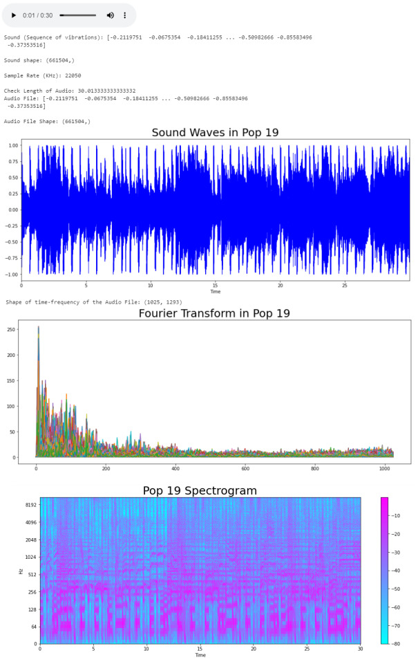
Audio Features
Now that we know what the audio data looks like to python, we can proceed to extract the Audio Features. The features we will need to extract, based on the provided CSV, are: · Harmonics · Percussion · Zero Crossing Rate · Tempo · Spectral Centroid · Spectral Rollof · Mel-Frequency Cepstral Coefficients · Chroma Frequencies Let’s start with the Harmonics and Percussive components:
# Decompose the Harmonics and Percussive components and show Representation
y_harm, y_perc = librosa.effects.hpss(audio_file)
plt.figure(figsize = (16, 6))
plt.plot(y_harm, color = 'g');
plt.plot(y_perc, color = 'm');
plt.title("Harmonics and Percussive components", fontsize = 25);
Using the librosa.effects.hpss function, we are able to separate the harmonics and percussive elements from the audio source and plot it into a visual representation.
Now we can retrieve the Zero Crossing Rate, using the librosa.zero_crossings function.
> Zero Crossing Rate: The rate of sign-changes (the number of times the signal changes value) of the audio signal during the frame.
#Total number of zero crossings
zero_crossings = librosa.zero_crossings(audio_file, pad=False)
print(sum(zero_crossings))
The Tempo (Beats per Minute) can be retrieved using the librosa.beat.beat_track function.
# Retrieving the Tempo in Pop 19
tempo, _ = librosa.beat.beat_track(y, sr = sr)
print('Tempo:', tempo , '\n')
The next feature extracted is the Spectral Centroids. > Spectral Centroid: a measure used in digital signal processing to characterize a spectrum. It determines the frequency area around which most of the signal energy concentrates.
# Calculate the Spectral Centroids
spectral_centroids = librosa.feature.spectral_centroid(audio_file, sr=sr)[0]
print('Centroids:', spectral_centroids, '\n')
print('Shape of Spectral Centroids:', spectral_centroids.shape, '\n')
# Computing the time variable for visualization
frames = range(len(spectral_centroids))
# Converts frame counts to time (seconds)
t = librosa.frames_to_time(frames)
print('Frames:', frames, '\n')
print('Time:', t)
Now that we have the shape of the spectral centroids as an array and the time variable (from frame counts), we need to create a function that normalizes the data. Normalization is a technique used to adjust the volume of audio files to a standard level which allows the file to be processed clearly. Once it’s normalized we proceed to retrieve the Spectral Rolloff.
> Spectral Rolloff: the frequency under which the cutoff of the total energy of the spectrum is contained, used to distinguish between sounds. The measure of the shape of the signal.
# Function that normalizes the Sound Data
def normalize(x, axis=0):
return sklearn.preprocessing.minmax_scale(x, axis=axis)
# Spectral RollOff Vector
spectral_rolloff = librosa.feature.spectral_rolloff(audio_file, sr=sr)[0]
plt.figure(figsize = (16, 6))
librosa.display.waveplot(audio_file, sr=sr, alpha=0.4, color = '#A300F9');
plt.plot(t, normalize(spectral_rolloff), color='#FFB100');
Using the audio file, we can continue to get the Mel-Frequency Cepstral Coefficients, which are a set of 20 features. In Music Information Retrieval, it’s often used to describe timbre. We will employ the librosa.feature.mfcc function.
mfccs = librosa.feature.mfcc(audio_file, sr=sr)
print('Mel-Frequency Ceptral Coefficient shape:', mfccs.shape)
#Displaying the Mel-Frequency Cepstral Coefficients:
plt.figure(figsize = (16, 6))
librosa.display.specshow(mfccs, sr=sr, x_axis='time', cmap = 'cool');
The MFCC shape is (20, 1,293), which means that the librosa.feature.mfcc function computed 20 coefficients over 1,293 frames.
mfccs = sklearn.preprocessing.scale(mfccs, axis=1)
print('Mean:', mfccs.mean(), '\n')
print('Var:', mfccs.var())
plt.figure(figsize = (16, 6))
librosa.display.specshow(mfccs, sr=sr, x_axis='time', cmap = 'cool');
Now we retrieve the Chroma Frequencies, using librosa.feature.chroma_stft. > Chroma Frequencies (or Features): are a powerful tool for analyzing music by categorizing pitches. These features capture harmonic and melodic characteristics of music.
# Increase or decrease hop_length to change how granular you want your data to be
hop_length = 5000
# Chromogram
chromagram = librosa.feature.chroma_stft(audio_file, sr=sr, hop_length=hop_length)
print('Chromogram shape:', chromagram.shape)
plt.figure(figsize=(16, 6))
librosa.display.specshow(chromagram, x_axis='time', y_axis='chroma', hop_length=hop_length, cmap='coolwarm');
The output:
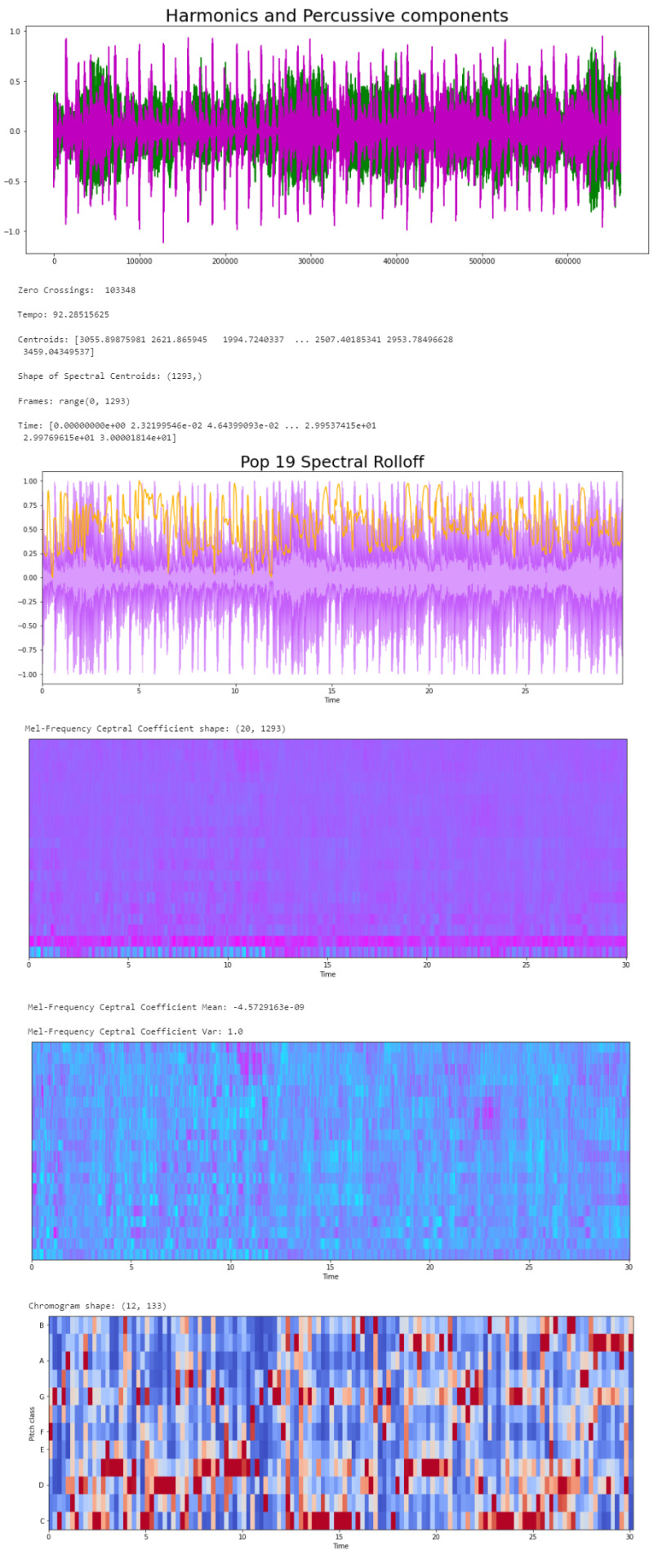
Exploratory Data Analysis
Now that we have a visual understanding of what an audio file looks like, and we’ve explored a good set of features, we can perform EDA, or Exploratory Data Analysis. This is all about getting to know the data and data profiling, summarizing the dataset through descriptive statistics. We can do this by getting a description of the data, using the describe() function or head() function. The describe() function will give us a description of all the dataset rows, and the head() function will give us the written data. We will perform EDA on the csv file, which contains all of the features previously analyzed above, and use the head() function:
# Loading the CSV file
data = pd.read_csv(f'{general_path}/features_30_sec.csv')
data.head()
Now we can create the correlation matrix of the data found in the csv file, using the feature means (average). We do this to summarize our data and pass it into a Correlation Heatmap.
# Computing the Correlation Matrix
spike_cols = [col for col in data.columns if 'mean' in col]
corr = data[spike_cols].corr()
The corr() function finds a pairwise correlation of all columns, excluding non-numeric and null values.
Now we can plot the heatmap:
# Generate a mask for the upper triangle
mask = np.triu(np.ones_like(corr, dtype=np.bool))
# Set up the matplotlib figure
f, ax = plt.subplots(figsize=(16, 11));
# Generate a custom diverging colormap
cmap = sns.diverging_palette(0, 25, as_cmap=True, s = 90, l = 45, n = 5)
# Draw the heatmap with the mask and correct aspect ratio
sns.heatmap(corr, mask=mask, cmap=cmap, vmax=.3, center=0,
square=True, linewidths=.5, cbar_kws={"shrink": .5}
plt.title('Correlation Heatmap (for the MEAN variables)', fontsize = 25)
plt.xticks(fontsize = 10)
plt.yticks(fontsize = 10);
Now we will take the data and, extracting the label(genre) and the tempo, we will draw a Box Plot. Box Plots visually show the distribution of numerical data through displaying percentiles and averages.
# Setting the axis for the box plot
x = data[["label", "tempo"]]
f, ax = plt.subplots(figsize=(16, 9));
sns.boxplot(x = "label", y = "tempo", data = x, palette = 'husl');
plt.title('Tempo(BPM) Boxplot for Genres', fontsize = 25)
plt.xticks(fontsize = 14)
plt.yticks(fontsize = 10);
plt.xlabel("Genre", fontsize = 15)
plt.ylabel("BPM", fontsize = 15)
Now we will draw a Scatter Diagram. To do this, we need to visualize possible groups of genres:
# To visualize possible groups of genres
data = data.iloc[0:, 1:]
y = data['label']
X = data.loc[:, data.columns != 'label']
We use data.iloc to get rows and columns at integer locations, and data.loc to get rows and columns with particular labels, excluding the label column. The next step is to normalize our data:
# Normalization
cols = X.columns
min_max_scaler = preprocessing.MinMaxScaler()
np_scaled = min_max_scaler.fit_transform(X)
X = pd.DataFrame(np_scaled, columns = cols)
Using the preprocessing library, we rescale each feature to a given range. Then we add a fit to data and transform (fit_transform).
We can proceed with a Principal Component Analysis:
# Principal Component Analysis
pca = PCA(n_components=2)
principalComponents = pca.fit_transform(X)
principalDf = pd.DataFrame(data = principalComponents, columns = ['principal component 1', 'principal component 2'])
# concatenate with target label
finalDf = pd.concat([principalDf, y], axis = 1)
PCA is used to reduce dimensionality in data. The fit learns some quantities from the data. Before the fit transform, the data shape was [1000, 58], meaning there’s 1000 rows with 58 columns (in the CSV file there’s 60 columns but two of these are string values, so it leaves with 58 numeric columns).
Once we use the PCA function, and set the components number to 2 we reduce the dimension of our project from 58 to 2. We have found the optimal stretch and rotation in our 58-dimension space to see the layout in two dimensions.
After reducing the dimensional space, we lose some variance(information).
pca.explained_variance_ratio_
By using this attribute we get the explained variance ratio, which we sum to get the percentage. In this case the variance explained is 46.53% .
plt.figure(figsize = (16, 9))
sns.scatterplot(x = "principal component 1", y = "principal component 2", data = finalDf, hue = "label", alpha = 0.7,
s = 100);
plt.title('PCA on Genres', fontsize = 25)
plt.xticks(fontsize = 14)
plt.yticks(fontsize = 10);
plt.xlabel("Principal Component 1", fontsize = 15)
plt.ylabel("Principal Component 2", fontsize = 15)
plt.savefig("PCA Scattert.jpg")
The output:
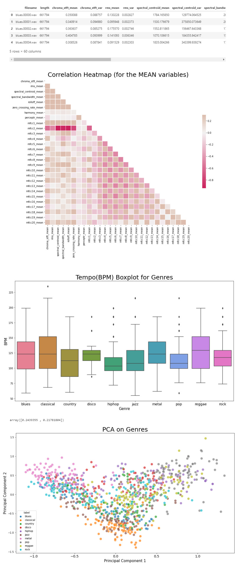
Genre Classification
Now we know what our data looks like, the features it has and have analyzed the principal component on all genres. All we have left to do is to build a classifier model that will predict any new audio data input its genre. We will use the CSV with 10 times the data for this.
# Load the data
data = pd.read_csv(f'{general_path}/features_3_sec.csv')
data = data.iloc[0:, 1:]
data.head()
Once again visualizing and normalizing the data.
y = data['label'] # genre variable.
X = data.loc[:, data.columns != 'label'] #select all columns but not the labels
# Normalization
cols = X.columns
min_max_scaler = preprocessing.MinMaxScaler()
np_scaled = min_max_scaler.fit_transform(X)
# new data frame with the new scaled data.
X = pd.DataFrame(np_scaled, columns = cols)
Now we have to split the data for training. Like I did in my previous post, the proportions are (70:30). 70% of the data will be used for training and 30% of the data will be used for testing.
# Split the data for training
X_train, X_test, y_train, y_test = train_test_split(X, y, test_size=0.3, random_state=42)
I tested 7 algorithms but I decided to go with K Nearest-Neighbors because I had previously used it.
knn = KNeighborsClassifier(n_neighbors=19)
knn.fit(X_train, y_train)
preds = knn.predict(X_test)
print('Accuracy', ':', round(accuracy_score(y_test, preds), 5), '\n')
# Confusion Matrix
confusion_matr = confusion_matrix(y_test, preds) #normalize = 'true'
plt.figure(figsize = (16, 9))
sns.heatmap(confusion_matr, cmap="Blues", annot=True,
xticklabels = ["blues", "classical", "country", "disco", "hiphop", "jazz", "metal", "pop", "reggae", "rock"],
yticklabels=["blues", "classical", "country", "disco", "hiphop", "jazz", "metal", "pop", "reggae", "rock"]);
The output:
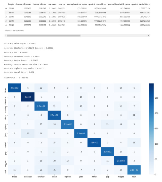
youtube
References
· https://medium.com/@james_52456/machine-learning-and-the-future-of-music-an-era-of-ml-artists-9be5ef27b83e
· https://www.kaggle.com/andradaolteanu/work-w-audio-data-visualise-classify-recommend/
· https://www.kaggle.com/dapy15/music-genre-classification/notebook
· https://towardsdatascience.com/how-to-start-implementing-machine-learning-to-music-4bd2edccce1f
· https://en.wikipedia.org/wiki/Music_information_retrieval
· https://pandas.pydata.org
· https://scikit-learn.org/
· https://seaborn.pydata.org
· https://matplotlib.org
· https://librosa.org/doc/main/index.html
· https://github.com/dmlc/xgboost
· https://docs.python.org/3/library/os.html
· https://www.tensorflow.org/
· https://www.hindawi.com/journals/sp/2021/1651560/
0 notes