#set row names in pandas dataframe | Explore Tumblr posts and blogs

ntaylor33 · 2 months ago

Text

Data Visualization - Assignment 2

For my first Python program, please see below:

-----------------------------PROGRAM--------------------------------

-- coding: utf-8 --

""" Created: 27FEB2025

@author:Nicole taylor """ import pandas import numpy

any additional libraries would be imported here

data = pandas.read_csv('GapFinder- _PDS.csv', low_memory=False)

print (len(data)) #number of observations (rows) print (len(data.columns)) # number of variables (columns)

checking the format of your variables

data['ref_area.label'].dtype

setting variables you will be working with to numeric

data['obs_value'] = pandas.to_numeric(data['obs_value'])

counts and percentages (i.e. frequency distributions) for each variable

Value1 = data['obs_value'].value_counts(sort=False) print (Value1)

PValue1 = data['obs_value'].value_counts(sort=False, normalize=True) print (PValue1)

Gender = data['sex.label'].value_counts(sort=False) print (Gender)

PGender = data['sex.label'].value_counts(sort=False, normalize=True) print (PGender)

Country = data['Country.label'].value_counts(sort=False) print (Country)

PCountry = data['Country.label'].value_counts(sort=False, normalize=True) print (PCountry)

MStatus = data['MaritalStatus.label'].value_counts(sort=False) print (MStatus)

PMStatus = data['MaritalStatus.label'].value_counts(sort=False, normalize=True) print (PMStatus)

LMarket = data['LaborMarket.label'].value_counts(sort=False) print (LMarket)

PLMarket = data['LaborMarket.label'].value_counts(sort=False, normalize=True) print (PLMarket)

Year = data['Year.label'].value_counts(sort=False) print (Year)

PYear = data['Year.label'].value_counts(sort=False, normalize=True) print (PYear)

ADDING TITLES

print ('counts for Value') Value1 = data['obs_value'].value_counts(sort=False) print (Value1)

print (len(data['TAB12MDX'])) #number of observations (rows)

print ('percentages for Value') p1 = data['obs_value'].value_counts(sort=False, normalize=True) print (PValue1)

print ('counts for Gender') Gender = data['sex.label'].value_counts(sort=False) print(Gender)

print ('percentages for Gender') p2 = data['sex.label'].value_counts(sort=False, normalize=True) print (PGender)

print ('counts for Country') Country = data['Country.label'].value_counts(sort=False, dropna=False) print(Country)

print ('percentages for Country') PCountry = data['Country.label'].value_counts(sort=False, normalize=True) print (PCountry)

print ('counts for Marital Status') MStatus = data['MaritalStatus.label'].value_counts(sort=False, dropna=False) print(MStatus)

print ('percentages for Marital Status') PMStatus = data['MaritalStatus.label'].value_counts(sort=False, dropna=False, normalize=True) print (PMStatus)

print ('counts for Labor Market') LMarket = data['LaborMarket.label'].value_counts(sort=False, dropna=False) print(LMarket)

print ('percentages for Labor Market') PLMarket = data['LaborMarket.label'].value_counts(sort=False, dropna=False, normalize=True) print (PLMarket)

print ('counts for Year') Year = data['Year.label'].value_counts(sort=False, dropna=False) print(Year)

print ('percentages for Year') PYear = data['Year.label'].value_counts(sort=False, dropna=False, normalize=True) print (PYear)

---------------------------------------------------------------------------

frequency distributions using the 'bygroup' function

print ('Frequency of Countries') TCountry = data.groupby('Country.label').size() print(TCountry)

subset data to young adults age 18 to 25 who have smoked in the past 12 months

sub1=data[(data[TCountry]='United States of America') & (data[Gender]='Sex:Female')]

make a copy of my new subsetted data

sub2 = sub1.copy()

frequency distributions on new sub2 data frame

print('counts for Country')

c5 = sub1['Country.label'].value_counts(sort=False)

print(c5)

upper-case all DataFrame column names - place afer code for loading data aboave

data.columns = list(map(str.upper, data.columns))

bug fix for display formats to avoid run time errors - put after code for loading data above

pandas.set_option('display.float_format', lambda x:'%f'%x)

-----------------------------RESULTS--------------------------------

runcell(0, 'C:/Users/oen8fh/.spyder-py3/temp.py') 85856 12 16372.131 1 7679.474 1 462.411 1 8230.246 1 4758.121 1 .. 1609.572 1 95.113 1 372.197 1 8.814 1 3.796 1 Name: obs_value, Length: 79983, dtype: int64

16372.131 0.000012 7679.474 0.000012 462.411 0.000012 8230.246 0.000012 4758.121 0.000012

1609.572 0.000012 95.113 0.000012 372.197 0.000012 8.814 0.000012 3.796 0.000012 Name: obs_value, Length: 79983, dtype: float64

Sex: Total 28595 Sex: Male 28592 Sex: Female 28595 Sex: Other 74 Name: sex.label, dtype: int64 Sex: Total 0.333058 Sex: Male 0.333023 Sex: Female 0.333058 Sex: Other 0.000862 Name: sex.label, dtype: float64 Afghanistan 210 Angola 291 Albania 696 Argentina 768 Armenia 627

Samoa 117 Yemen 36 South Africa 993 Zambia 306 Zimbabwe 261 Name: Country.label, Length: 169, dtype: int64

Afghanistan 0.002446 Angola 0.003389 Albania 0.008107 Argentina 0.008945 Armenia 0.007303

Samoa 0.001363 Yemen 0.000419 South Africa 0.011566 Zambia 0.003564 Zimbabwe 0.003040 Name: Country.label, Length: 169, dtype: float64

Marital status (Aggregate): Total 26164 Marital status (Aggregate): Single / Widowed / Divorced 26161 Marital status (Aggregate): Married / Union / Cohabiting 26156 Marital status (Aggregate): Not elsewhere classified 7375 Name: MaritalStatus.label, dtype: int64

Marital status (Aggregate): Total 0.304743 Marital status (Aggregate): Single / Widowed / Divorced 0.304708 Marital status (Aggregate): Married / Union / Cohabiting 0.304650 Marital status (Aggregate): Not elsewhere classified 0.085900 Name: MaritalStatus.label, dtype: float64

Labour market status: Total 21870 Labour market status: Employed 21540 Labour market status: Unemployed 20736 Labour market status: Outside the labour force 21710 Name: LaborMarket.label, dtype: int64

Labour market status: Total 0.254729 Labour market status: Employed 0.250885 Labour market status: Unemployed 0.241521 Labour market status: Outside the labour force 0.252865 Name: LaborMarket.label, dtype: float64

2021 3186 2020 3641 2017 4125 2014 4014 2012 3654 2022 3311 2019 4552 2011 3522 2009 3054 2004 2085 2023 2424 2018 3872 2016 3843 2015 3654 2013 3531 2010 3416 2008 2688 2007 2613 2005 2673 2002 1935 2006 2700 2024 372 2003 2064 2001 1943 2000 1887 1999 1416 1998 1224 1997 1086 1996 999 1995 810 1994 714 1993 543 1992 537 1991 594 1990 498 1989 462 1988 423 1987 423 1986 357 1985 315 1984 273 1983 309 1982 36 1980 36 1970 42 Name: Year.label, dtype: int64

2021 0.037109 2020 0.042408 2017 0.048046 2014 0.046753 2012 0.042560 2022 0.038565 2019 0.053019 2011 0.041022 2009 0.035571 2004 0.024285 2023 0.028233 2018 0.045099 2016 0.044761 2015 0.042560 2013 0.041127 2010 0.039788 2008 0.031308 2007 0.030435 2005 0.031134 2002 0.022538 2006 0.031448 2024 0.004333 2003 0.024040 2001 0.022631 2000 0.021979 1999 0.016493 1998 0.014256 1997 0.012649 1996 0.011636 1995 0.009434 1994 0.008316 1993 0.006325 1992 0.006255 1991 0.006919 1990 0.005800 1989 0.005381 1988 0.004927 1987 0.004927 1986 0.004158 1985 0.003669 1984 0.003180 1983 0.003599 1982 0.000419 1980 0.000419 1970 0.000489 Name: Year.label, dtype: float64

counts for Value 16372.131 1 7679.474 1 462.411 1 8230.246 1 4758.121 1 .. 1609.572 1 95.113 1 372.197 1 8.814 1 3.796 1 Name: obs_value, Length: 79983, dtype: int64

percentages for Value 16372.131 0.000012 7679.474 0.000012 462.411 0.000012 8230.246 0.000012 4758.121 0.000012

1609.572 0.000012 95.113 0.000012 372.197 0.000012 8.814 0.000012 3.796 0.000012 Name: obs_value, Length: 79983, dtype: float64

counts for Gender Sex: Total 28595 Sex: Male 28592 Sex: Female 28595 Sex: Other 74 Name: sex.label, dtype: int64

percentages for Gender Sex: Total 0.333058 Sex: Male 0.333023 Sex: Female 0.333058 Sex: Other 0.000862 Name: sex.label, dtype: float64

counts for Country Afghanistan 210 Angola 291 Albania 696 Argentina 768 Armenia 627

Samoa 117 Yemen 36 South Africa 993 Zambia 306 Zimbabwe 261 Name: Country.label, Length: 169, dtype: int64

percentages for Country Afghanistan 0.002446 Angola 0.003389 Albania 0.008107 Argentina 0.008945 Armenia 0.007303

Samoa 0.001363 Yemen 0.000419 South Africa 0.011566 Zambia 0.003564 Zimbabwe 0.003040 Name: Country.label, Length: 169, dtype: float64

counts for Marital Status Marital status (Aggregate): Total 26164 Marital status (Aggregate): Single / Widowed / Divorced 26161 Marital status (Aggregate): Married / Union / Cohabiting 26156 Marital status (Aggregate): Not elsewhere classified 7375 Name: MaritalStatus.label, dtype: int64

percentages for Marital Status Marital status (Aggregate): Total 0.304743 Marital status (Aggregate): Single / Widowed / Divorced 0.304708 Marital status (Aggregate): Married / Union / Cohabiting 0.304650 Marital status (Aggregate): Not elsewhere classified 0.085900 Name: MaritalStatus.label, dtype: float64

counts for Labor Market Labour market status: Total 21870 Labour market status: Employed 21540 Labour market status: Unemployed 20736 Labour market status: Outside the labour force 21710 Name: LaborMarket.label, dtype: int64

percentages for Labor Market Labour market status: Total 0.254729 Labour market status: Employed 0.250885 Labour market status: Unemployed 0.241521 Labour market status: Outside the labour force 0.252865 Name: LaborMarket.label, dtype: float64

counts for Year 2021 3186 2020 3641 2017 4125 2014 4014 2012 3654 2022 3311 2019 4552 2011 3522 2009 3054 2004 2085 2023 2424 2018 3872 2016 3843 2015 3654 2013 3531 2010 3416 2008 2688 2007 2613 2005 2673 2002 1935 2006 2700 2024 372 2003 2064 2001 1943 2000 1887 1999 1416 1998 1224 1997 1086 1996 999 1995 810 1994 714 1993 543 1992 537 1991 594 1990 498 1989 462 1988 423 1987 423 1986 357 1985 315 1984 273 1983 309 1982 36 1980 36 1970 42 Name: Year.label, dtype: int64

percentages for Year 2021 0.037109 2020 0.042408 2017 0.048046 2014 0.046753 2012 0.042560 2022 0.038565 2019 0.053019 2011 0.041022 2009 0.035571 2004 0.024285 2023 0.028233 2018 0.045099 2016 0.044761 2015 0.042560 2013 0.041127 2010 0.039788 2008 0.031308 2007 0.030435 2005 0.031134 2002 0.022538 2006 0.031448 2024 0.004333 2003 0.024040 2001 0.022631 2000 0.021979 1999 0.016493 1998 0.014256 1997 0.012649 1996 0.011636 1995 0.009434 1994 0.008316 1993 0.006325 1992 0.006255 1991 0.006919 1990 0.005800 1989 0.005381 1988 0.004927 1987 0.004927 1986 0.004158 1985 0.003669 1984 0.003180 1983 0.003599 1982 0.000419 1980 0.000419 1970 0.000489 Name: Year.label, dtype: float64

Frequency of Countries Country.label Afghanistan 210 Albania 696 Angola 291 Antigua and Barbuda 87 Argentina 768

Viet Nam 639 Wallis and Futuna 117 Yemen 36 Zambia 306 Zimbabwe 261 Length: 169, dtype: int64

-----------------------------REVIEW--------------------------------

So as you can see in the results. I was able to show the Year, Marital Status, Labor Market, and the Country. I'm still a little hazy on the sub1, but overall it was a good basic start.

0 notes

govindhtech · 6 months ago

Text

BigQuery DataFrame And Gretel Verify Synthetic Data Privacy

It looked at how combining Gretel with BigQuery DataFrame simplifies synthetic data production while maintaining data privacy in the useful guide to synthetic data generation with Gretel and BigQuery DataFrames. In summary, BigQuery DataFrame is a Python client for BigQuery that offers analysis pushed down to BigQuery using pandas-compatible APIs.

Gretel provides an extensive toolkit for creating synthetic data using state-of-the-art machine learning methods, such as large language models (LLMs). An seamless workflow is made possible by this integration, which makes it simple for users to move data from BigQuery to Gretel and return the created results to BigQuery.

The technical elements of creating synthetic data to spur AI/ML innovation are covered in detail in this tutorial, along with tips for maintaining high data quality, protecting privacy, and adhering to privacy laws. In Part 1, to de-identify the data from a BigQuery patient records table, and in Part 2, it create synthetic data to be saved back to BigQuery.

Setting the stage: Installation and configuration

With BigFrames already installed, you may begin by using BigQuery Studio as the notebook runtime. To presume you are acquainted with Pandas and have a Google Cloud project set up.

Step 1: Set up BigQuery DataFrame and the Gretel Python client.

Step 2: Set up BigFrames and the Gretel SDK: To use their services, you will want a Gretel API key. One is available on the Gretel console.

Part 1: De-identifying and processing data with Gretel Transform v2

De-identifying personally identifiable information (PII) is an essential initial step in data anonymization before creating synthetic data. For these and other data processing tasks, Gretel Transform v2 (Tv2) offers a strong and expandable framework.

Tv2 handles huge datasets efficiently by combining named entity recognition (NER) skills with sophisticated transformation algorithms. Tv2 is a flexible tool in the data preparation pipeline as it may be used for preprocessing, formatting, and data cleaning in addition to PII de-identification. Study up on Gretel Transform v2.

Step 1: Convert your BigQuery table into a BigFrames DataFrame.

Step 2: Work with Gretel to transform the data.

Part 2: Generating synthetic data with Navigator Fine Tuning (LLM-based)

Gretel Navigator Fine Tuning (NavFT) refines pre-trained models on your datasets to provide high-quality, domain-specific synthetic data. Important characteristics include:

Manages a variety of data formats, including time series, JSON, free text, category, and numerical.

Maintains intricate connections between rows and data kinds.

May provide significant novel patterns, which might enhance the performance of ML/AI tasks.

Combines privacy protection with data usefulness.

By utilizing the advantages of domain-specific pre-trained models, NavFT expands on Gretel Navigator’s capabilities and makes it possible to create synthetic data that captures the subtleties of your particular data, such as the distributions and correlations for numeric, categorical, and other column types.

Using the de-identified data from Part 1, it will refine a Gretel model in this example.

Step 1: Make a model better:

# Display the full report within this notebooktrain_results.report.display_in_notebook()

Step 2: Retrieve the Quality Report for Gretel Synthetic Data.

Step 3: Create synthetic data using the optimized model, assess the privacy and quality of the data, and then publish the results back to a BQ table.

A few things to note about the synthetic data:

Semantically accurate, the different modalities (free text, JSON structures) are completely synthetic and retained.

The data are grouped by patient during creation due to the group-by/order-by hyperparameters that were used during fine-tuning.

How to use BigQuery with Gretel

This technical manual offers a starting point for creating and using synthetic data using Gretel AI and BigQuery DataFrame. You may use the potential of synthetic data to improve your data science, analytics, and artificial intelligence development processes while maintaining data privacy and compliance by examining the Gretel documentation and using these examples.

Read more on Govindhtech.com

#BigQueryDataFrame #DataFrame #Gretel #AI #ML #Python #SyntheticData #cloudcomputing #BigQuery #News #Technews #Technology #Technologynews #Technologytrends #govindhtech

0 notes

youngtigercheesecake · 1 year ago

Text

week 2:

Assignment : Running Your First Program

import pandas import numpy

data = pandas.read_csv('addhealth_pds.csv', low_memory=False)

print (len(data)) #number of observations (rows) print (len(data.columns)) # number of variables (columns)

setting variables you will be working with to numeric

data['BIO_SEX'] = pandas.to_numeric(data['BIO_SEX']) data['H1SU1'] = pandas.to_numeric(data['H1SU1']) data['H1SU2'] = pandas.to_numeric(data['H1SU2']) data['H1TO14'] = pandas.to_numeric(data['H1TO14'])

counts and percentages (i.e. frequency distributions) for each variable

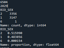
c1 = data['BIO_SEX'].value_counts(sort=False) print (c1)

p1 = data['BIO_SEX'].value_counts(sort=False, normalize=True) print (p1)

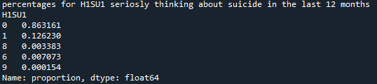
c2 = data['H1SU1'].value_counts(sort=False) print(c2)

p2 = data['H1SU1'].value_counts(sort=False, normalize=True) print (p2)

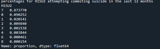
c3 = data['H1SU2'].value_counts(sort=False) print(c3)

p3 = data['H1SU2'].value_counts(sort=False, normalize=True) print (p3)

c4 = data['H1TO15'].value_counts(sort=False) print(c4)

ADDING TITLES

print ('counts for BIO_SEX') c1 = data['BIO_SEX'].value_counts(sort=False) print (c1)

print (len(data['BIO_SEX'])) #number of observations (rows)

print ('percentages for BIO_SEX') p1 = data['BIO_SEX'].value_counts(sort=False, normalize=True) print (p1)

print ('counts for H1SU1') c2 = data['H1SU1'].value_counts(sort=False) print(c2)

print ('percentages for H1SU1') p2 = data['H1SU1'].value_counts(sort=False, normalize=True) print (p2)

print ('counts for H1SU2') c3 = data['H1SU2'].value_counts(sort=False, dropna=False) print(c3)

print ('percentages for H1SU2') p3 = data['H1SU2'].value_counts(sort=False, normalize=True) print (p3)

print ('counts for H1TO15') c4 = data['H1TO15'].value_counts(sort=False, dropna=False) print(c4)

print ('percentages for H1TO15') p4 = data['H1TO15'].value_counts(sort=False, dropna=False, normalize=True) print (p4)

ADDING MORE DESCRIPTIVE TITLES

print('counts for BIO_SEX“ what is the gender') c1 = data['BIO_SEX'].value_counts(sort=False) print (c1)

print('percentages for BIO_SEX what is the gender') p1 = data['BIO_SEX'].value_counts(sort=False, normalize=True) print (p1)

print('counts for H1SU1 seriosly thinking about suicide in the last 12 months') c2 = data['H1SU1'].value_counts(sort=False) print(c2)

print('percentages for H1SU1 seriosly thinking about suicide in the last 12 months') p2 = data['H1SU1'].value_counts(sort=False, normalize=True) print (p2)

print('counts for H1SU2 attempting commiting suicide in the last 12 months') c3 = data['H1SU2'].value_counts(sort=False) print(c3)

print('percentages for H1SU2 attempting commiting suicide in the last 12 months') p3 = data['H1SU2'].value_counts(sort=False, normalize=True) print (p3)

print('counts for H1TO15 how many times a person thinks about alcohol during the past 12 months') c4 = data['H1TO15'].value_counts(sort=False, dropna=False) print(c4)

print('percentages for H1TO15 how many times a person thinks about alcohol during the past 12 months') p4 = data['H1TO15'].value_counts(sort=False, normalize=True) print (p4)

frequency distributions using the 'bygroup' function

ct1= data.groupby('BIO_SEX').size() print(ct1)

pt1 = data.groupby('BIO_SEX').size() * 100 / len(data) print(pt1)

subset data to male attempting commiting suicide in the last 12 months

sub1=data[(data['BIO_SEX']==1) & (data['H1SU1']==1)]

make a copy of my new subsetted data

sub2 = sub1.copy()

frequency distributions on new sub2 data frame

print('counts for BIO_SEX') c5 = sub2['BIO_SEX'].value_counts(sort=False) print(c5)

print('percentages for BIO_SEX') p5 = sub2['BIO_SEX'].value_counts(sort=False, normalize=True) print (p5)

print('counts for H1SU1') c6 = sub2['H1TO13'].value_counts(sort=False) print(c6)

print('percentages for H1SU1') p6 = sub2['H1SU1'].value_counts(sort=False, normalize=True) print (p6)

upper-case all DataFrame column names - place afer code for loading data aboave

data.columns = list(map(str.upper, data.columns))

bug fix for display formats to avoid run time errors - put after code for loading data above

pandas.set_option('display.float_format', lambda x:'%f'%x) Results: In this part we see how many male, how many female and undefined respondents there are, and what is that number expressed in percentages

Refining research question:

Research question is how many men seriously thought about committing suicide in the previous 12 months?

0 notes

edcater · 1 year ago

Text

Embarking on Your Data Science Journey: A Beginner's Guide

Are you intrigued by the world of data, eager to uncover insights hidden within vast datasets? If so, welcome to the exciting realm of data science! At the heart of this field lies Python programming, a versatile and powerful tool that enables you to manipulate, analyze, and visualize data. Whether you're a complete beginner or someone looking to expand their skill set, this guide will walk you through the basics of Python programming for data science in simple, easy-to-understand terms.

1. Understanding Data Science and Python

Before we delve into the specifics, let's clarify what data science is all about. Data science involves extracting meaningful information and knowledge from large, complex datasets. This information can then be used to make informed decisions, predict trends, and gain valuable insights.

Python, a popular programming language, has become the go-to choice for data scientists due to its simplicity, readability, and extensive libraries tailored for data manipulation and analysis.

2. Installing Python

The first step in your data science journey is to install Python on your computer. Fortunately, Python is free and can be easily downloaded from the official website, python.org. Choose the version compatible with your operating system (Windows, macOS, or Linux) and follow the installation instructions.

3. Introduction to Jupyter Notebooks

While Python can be run from the command line, using Jupyter Notebooks is highly recommended for data science projects. Jupyter Notebooks provide an interactive environment where you can write and execute Python code in a more user-friendly manner. To install Jupyter Notebooks, use the command pip install jupyterlab in your terminal or command prompt.

4. Your First Python Program

Let's create your very first Python program! Open a new Jupyter Notebook and type the following code:

python

Copy code

print("Hello, Data Science!")

To execute the code, press Shift + Enter. You should see the phrase "Hello, Data Science!" printed below the code cell. Congratulations! You've just run your first Python program.

5. Variables and Data Types

In Python, variables are used to store data. Here are some basic data types you'll encounter:

Integers: Whole numbers, such as 1, 10, or -5.

Floats: Numbers with decimals, like 3.14 or -0.001.

Strings: Text enclosed in single or double quotes, such as "Hello" or 'Python'.

Booleans: True or False values.

To create a variable, simply assign a value to a name. For example:

python

Copy code

age = 25

name = "Alice"

is_student = True

6. Working with Lists and Dictionaries

Lists and dictionaries are essential data structures in Python. A list is an ordered collection of items, while a dictionary is a collection of key-value pairs.

Lists:

python

Copy code

fruits = ["apple", "banana", "cherry"]

print(fruits[0]) # Accessing the first item

fruits.append("orange") # Adding a new item

Dictionaries:

python

Copy code

person = {"name": "John", "age": 30, "is_student": False}

print(person["name"]) # Accessing value by key

person["city"] = "New York" # Adding a new key-value pair

7. Basic Data Analysis with Pandas

Pandas is a powerful library for data manipulation and analysis in Python. Let's say you have a dataset in a CSV file called data.csv. You can load and explore this data using Pandas:

python

Copy code

import pandas as pd

# Load the data into a DataFrame

df = pd.read_csv("data.csv")

# Display the first few rows of the DataFrame

print(df.head())

8. Visualizing Data with Matplotlib

Matplotlib is a versatile library for creating various types of plots and visualizations. Here's an example of creating a simple line plot:

python

Copy code

import matplotlib.pyplot as plt

# Data for plotting

x = [1, 2, 3, 4, 5]

y = [2, 4, 6, 8, 10]

# Create a line plot

plt.plot(x, y)

plt.xlabel('X-axis')

plt.ylabel('Y-axis')

plt.title('Simple Line Plot')

plt.show()

9. Further Learning and Resources

As you continue your data science journey, there are countless resources available to deepen your understanding of Python and its applications in data analysis. Here are a few recommendations:

Online Courses: Platforms like Coursera, Udemy, and DataCamp offer beginner-friendly courses on Python for data science.

Books: "Python for Data Analysis" by Wes McKinney and "Automate the Boring Stuff with Python" by Al Sweigart are highly recommended.

Practice: The best way to solidify your skills is to practice regularly. Try working on small projects or participating in Kaggle competitions.

Conclusion

Embarking on a journey into data science with Python is an exciting and rewarding endeavor. By mastering the basics covered in this guide, you've laid a strong foundation for exploring the vast landscape of data analysis, visualization, and machine learning. Remember, patience and persistence are key as you navigate through datasets and algorithms. Happy coding, and may your data science adventures be fruitful!

0 notes

chieffurycollection · 2 years ago

Text

Linear regression alcohol consumption vs number of alcoholic parents

Code

import pandas import numpy import matplotlib.pyplot as plt from sklearn.linear_model import LinearRegression from sklearn.model_selection import train_test_split from sklearn.metrics import mean_squared_error, r2_score import statsmodels.api as sm import seaborn import statsmodels.formula.api as smf

print("start import") data = pandas.read_csv('nesarc_pds.csv', low_memory=False) print("import done")

upper-case all Dataframe column names --> unification

data.colums = map(str.upper, data.columns)

bug fix for display formats to avoid run time errors

pandas.set_option('display.float_format', lambda x:'%f'%x)

print (len(data)) #number of observations (rows) print (len(data.columns)) # number of variables (columns)

checking the format of your variables

setting variables you will be working with to numeric

data['S2DQ1'] = pandas.to_numeric(data['S2DQ1']) #Blood/Natural Father data['S2DQ2'] = pandas.to_numeric(data['S2DQ2']) #Blood/Natural Mother data['S2BQ3A'] = pandas.to_numeric(data['S2BQ3A'], errors='coerce') #Age at first Alcohol abuse data['S3CQ14A3'] = pandas.to_numeric(data['S3CQ14A3'], errors='coerce')

Blood/Natural Father was alcoholic

print("number blood/natural father was alcoholic")

0 = no; 1= yes; unknown = nan

data['S2DQ1'] = data['S2DQ1'].replace({2: 0, 9: numpy.nan}) c1 = data['S2DQ1'].value_counts(sort=False).sort_index() print (c1)

print("percentage blood/natural father was alcoholic") p1 = data['S2DQ1'].value_counts(sort=False, normalize=True).sort_index() print (p1)

Blood/Natural Mother was alcoholic

print("number blood/natural mother was alcoholic")

0 = no; 1= yes; unknown = nan

data['S2DQ2'] = data['S2DQ2'].replace({2: 0, 9: numpy.nan}) c2 = data['S2DQ2'].value_counts(sort=False).sort_index() print(c2)

print("percentage blood/natural mother was alcoholic") p2 = data['S2DQ2'].value_counts(sort=False, normalize=True).sort_index() print (p2)

Data Management: Number of parents with background of alcoholism is calculated

0 = no parents; 1 = at least 1 parent (maybe one answer missing); 2 = 2 parents; nan = 1 unknown and 1 zero or both unknown

print("number blood/natural parents was alcoholic") data['Num_alcoholic_parents'] = numpy.where((data['S2DQ1'] == 1) & (data['S2DQ2'] == 1), 2, numpy.where((data['S2DQ1'] == 1) & (data['S2DQ2'] == 0), 1, numpy.where((data['S2DQ1'] == 0) & (data['S2DQ2'].isna()), numpy.nan, numpy.where((data['S2DQ1'] == 0) & (data['S2DQ2'].isna()), numpy.nan, numpy.where((data['S2DQ1'] == 0) & (data['S2DQ2'] == 0), 0, numpy.nan)))))

c5 = data['Num_alcoholic_parents'].value_counts(sort=False).sort_index() print(c5)

print("percentage blood/natural parents was alcoholic") p5 = data['Num_alcoholic_parents'].value_counts(sort=False, normalize=True).sort_index() print (p5)

___________________________________________________________________Graphs_________________________________________________________________________

Diagramm für c5 erstellen

plt.figure(figsize=(8, 5)) plt.bar(c5.index, c5.values) plt.xlabel('Num_alcoholic_parents') plt.ylabel('Häufigkeit') plt.title('Häufigkeitsverteilung von Num_alcoholic_parents') plt.xticks(c5.index) plt.show()

Diagramm für p5 erstellen

plt.figure(figsize=(8, 5)) plt.bar(p5.index, p5.values*100) plt.xlabel('Num_alcoholic_parents') plt.ylabel('Häufigkeit (%)') plt.title('Häufigkeitsverteilung von Num_alcoholic_parents') plt.xticks(c5.index) plt.show()

print("lineare Regression")

Entfernen Sie Zeilen mit NaN-Werten in den relevanten Spalten.

data_cleaned = data.dropna(subset=['Num_alcoholic_parents', 'S2BQ3A'])

Definieren Sie Ihre unabhängige Variable (X) und Ihre abhängige Variable (y).

X = data_cleaned['Num_alcoholic_parents'] y = data_cleaned['S2BQ3A']

Fügen Sie eine Konstante hinzu, um den Intercept zu berechnen.

X = sm.add_constant(X)

Erstellen Sie das lineare Regressionsmodell.

model = sm.OLS(y, X).fit()

Drucken Sie die Zusammenfassung des Modells.

print(model.summary()) Result

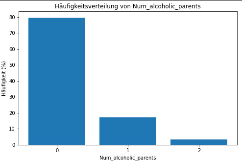
frequency distribution shows how many of the people from the study have alcoholic parents and if its only 1 oder both parents.

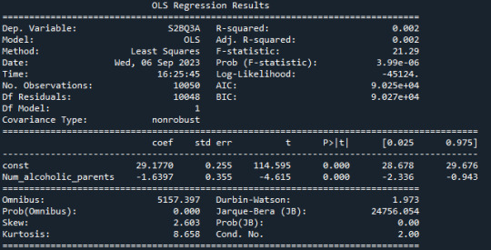
R-squared: The R-squared value is 0.002, indicating that only about 0.2% of the variation in "S2BQ3A" (quantity of alcoholic drinks consumed) is explained by the variable "Num_alcoholic_parents" (number of alcoholic parents). This suggests that there is likely no strong linear relationship between these two variables.

F-statistic: The F-statistic has a value of 21.29, and the associated probability (Prob (F-statistic)) is very small (3.99e-06). The F-statistic is used to assess the overall effectiveness of the model. In this case, the low probability suggests that at least one of the independent variables has a significant impact on the dependent variable.

Coefficients: The coefficients of the model show the estimated effects of the independent variables on the dependent variable. In this case, the constant (const) has a value of 29.1770, representing the estimated average value of "S2BQ3A" when "Num_alcoholic_parents" is zero. The coefficient for "Num_alcoholic_parents" is -1.6397, meaning that an additional alcoholic parent is associated with an average decrease of 1.6397 units in "S2BQ3A" (quantity of alcoholic drinks consumed).

P-Values (P>|t|): The p-values next to the coefficients indicate the significance of each coefficient. In this case, both the constant and the coefficient for "Num_alcoholic_parents" are highly significant (p-values close to zero). This suggests that "Num_alcoholic_parents" has a statistically significant impact on "S2BQ3A."

AIC and BIC: AIC (Akaike Information Criterion) and BIC (Bayesian Information Criterion) are model evaluation measures. Lower values indicate a better model fit. In this case, both AIC and BIC are relatively low, which could indicate the adequacy of the model.

In summary, there is a statistically significant but very weak negative relationship between the number of alcoholic parents and the quantity of alcoholic drinks consumed. This means that an increase in the number of alcoholic parents is associated with a slight decrease in the quantity of alcohol consumed, but it explains only a very limited amount of the variation in the quantity of alcohol consumed.

0 notes

analysisbyzee · 4 years ago

Text

Classification Decision Tree for Heart Attack Analysis

Primarily, the required dataset is loaded. Here, I have uploaded the dataset available at Kaggle.com in the csv format.

All python libraries need to be loaded that are required in creation for a classification decision tree. Following are the libraries that are necessary to import:

The following code is used to load the dataset. read_csv() function is used to load the dataset.

column_names = ['age','sex','chest pain','resting blood pressure','cholestrol','fasting blood sugar','resting ecg','max heart rate','excercise included','old peak','slp','caa','THALL','output']

data= pd.read_csv("heart.csv",header=None,names=column_names)

data = data.iloc[1: , :] # removes the first row of dataframe

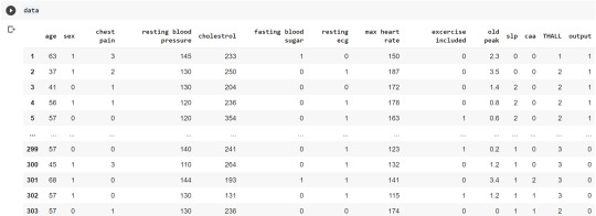
Now, we divide the columns in the dataset as dependent or independent variables. The output variable is selected as target variable for heart disease prediction system. The dataset contains 13 feature variables and 1 target variable.

feature_cols = ['age','sex','chest pain','chest pain','resting blood pressure','cholestrol','fasting blood sugar','resting ecg','max heart rate','excercise included','old peak','slp','caa','THALL']

pred = data[feature_cols] # Features

tar = data.output # Target variable

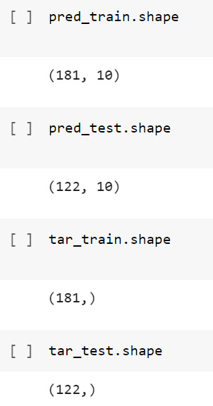
Now, dataset is divided into a training set and a test set. This can be achieved by using train_test_split() function. The size ratio is set as 60% for the training sample and 40% for the test sample.

pred_train, pred_test, tar_train, tar_test = train_test_split(X, y, test_size=0.4, random_state=1)

Using the shape function, we observe that the training sample has 181 observations (nearly 60% of the original sample) and 10 explanatory variables whereas the test sample contains 122 observations(nearly 40 % of the original sample) and 10 explanatory variables.

Now, we need to create an object claf_mod to initialize the decision tree classifer. The model is then trained using the fit function which takes training features and training target variables as arguments.

# To create an object of Decision Tree classifer

claf_mod = DecisionTreeClassifier()

# Train the model

claf_mod = claf_mod.fit(pred_train,tar_train)

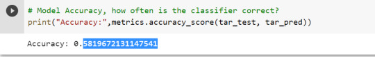
To check the accuracy of the model, we use the accuracy_score function of metrics library. Our model has a classification rate of 58.19 %. Therefore, we can say that our model has good accuracy for finding out a person has a heart attack.

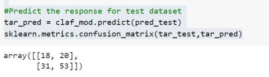
To find out the correct and incorrect classification of decision tree, we use the confusion matrix function. Our model predicted 18 true negatives for having a heart disease and 53 true positives for having a heart attack. The model also predicted 31 false negatives and 20 false positives for having a heart attack.

To display the decision tree we use export_graphviz function. The resultant graph is unpruned.

dot_data = StringIO()

export_graphviz(claf_mod, out_file=dot_data,

filled=True, rounded=True,

special_characters=True,class_names=['0','1'])

graph = pydotplus.graph_from_dot_data(dot_data.getvalue())

graph.write_png('heart attack.png')

Image(graph.create_png())

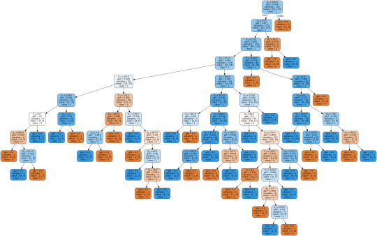
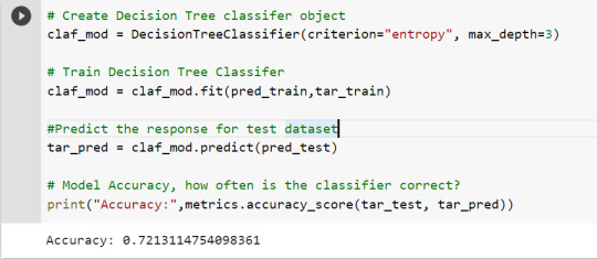
To get a prune graph, we changed the criterion as entropy and initialized the object again. The maximum depth of the tree is set as 3 to avoid overfitting.

# Create Decision Tree classifer object

claf_mod = DecisionTreeClassifier(criterion="entropy", max_depth=3)

# Train Decision Tree Classifer

claf_mod = claf_mod.fit(pred_train,tar_train)

#Predict the response for test dataset

tar_pred = claf_mod.predict(pred_test)

By optimizing the performance, the classification rate of the model increased to 72.13%.

By passing the object again into export_graphviz function, we obtain the prune graph.

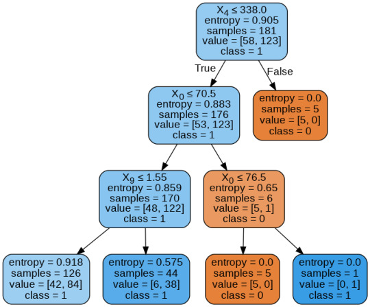
From the above graph, we can infer that :

1) individuals having cholesterol less than 338 mg/dl, age less than or equal to 70.5 years, and whose previous peak was less than or equal to 1.55: 84 of them are more likely to have a heart attack whereas 42 of them will less likely to have a heart attack.

2) individuals having cholesterol less than 338 mg/dl, age less than or equal to 70.5 years, and whose previous peak was more than 1.55: 6 of them will less likely to have a heart attack whereas 38 of them are more likely to have a heart attack.

3) individuals having cholesterol less than 338 mg/dl and age less than or equal to 76.5 years: are less likely to have a heart attack

4) individuals having cholesterol less than 338 mg/dl and age more than 76.5 years: are more likely to have a heart attack

5) individuals having cholesterol more than 338 mg/dl : are less likely to have a heart attack

The Whole Code:

from google.colab import files uploaded = files.upload()

import pandas as pd from sklearn.tree import DecisionTreeClassifier # Import Decision Tree Classifier from sklearn.model_selection import train_test_split # Import train_test_split function from sklearn.metrics import classification_report import sklearn.metrics #Import scikit-learn metrics module for accuracy calculation from sklearn.tree import export_graphviz from sklearn.externals.six import StringIO from IPython.display import Image import pydotplus

column_names = ['age','sex','chest pain','resting blood pressure','cholestrol','fasting blood sugar','resting ecg','max heart rate','excercise included','old peak','slp','caa','THALL','output'] data= pd.read_csv("heart.csv",header=None,names=column_names) data = data.iloc[1: , :] # removes the first row of dataframe (In this case, ) #split dataset in features and target variable feature_cols = ['age','sex','chest pain','chest pain','resting blood pressure','cholestrol','fasting blood sugar','resting ecg','max heart rate','excercise included','old peak','slp','caa','THALL'] pred = data[feature_cols] # Features tar = data.output # Target variable pred_train, pred_test, tar_train, tar_test = train_test_split(X, y, test_size=0.4, random_state=1) # 60% training and 40% test pred_train.shape pred_test.shape tar_train.shape tar_test.shape

# To create an object of Decision Tree classifer claf_mod = DecisionTreeClassifier() # Train the model claf_mod = claf_mod.fit(pred_train,tar_train) #Predict the response for test dataset tar_pred = claf_mod.predict(pred_test) sklearn.metrics.confusion_matrix(tar_test,tar_pred) # Model Accuracy, how often is the classifier correct? print("Accuracy:",metrics.accuracy_score(tar_test, tar_pred)) dot_data = StringIO() export_graphviz(claf_mod, out_file=dot_data, filled=True, rounded=True, special_characters=True,class_names=['0','1']) graph = pydotplus.graph_from_dot_data(dot_data.getvalue()) graph.write_png('heart attack.png') Image(graph.create_png())

# Create Decision Tree classifer object claf_mod = DecisionTreeClassifier(criterion="entropy", max_depth=3) # Train Decision Tree Classifer claf_mod = claf_mod.fit(pred_train,tar_train) #Predict the response for test dataset tar_pred = claf_mod.predict(pred_test) # Model Accuracy, how often is the classifier correct? print("Accuracy:",metrics.accuracy_score(tar_test, tar_pred)) from sklearn.externals.six import StringIO from IPython.display import Image from sklearn.tree import export_graphviz import pydotplus dot_data = StringIO() export_graphviz(claf_mod, out_file=dot_data, filled=True, rounded=True, special_characters=True, class_names=['0','1']) graph = pydotplus.graph_from_dot_data(dot_data.getvalue()) graph.write_png('improved heart attack.png') Image(graph.create_png())

#python #decision tree #heart attack #analysis #project #machine learning #data analysis

1 note · View note

21shubhamkhodape · 5 years ago

Text

Decision Tree

Machine Learning(ML):

Machine learning is an application of artificial intelligence (AI) that provides systems the ability to automatically learn and improve from experience without being explicitly programmed. Machine learning focuses on the development of computer programs that can access data and use it learn for themselves.It is the field of study that gives computers the capability to learn without being explicitly programmed. ML is one of the most exciting technologies that one would have ever come across. As it is evident from the name, it gives the computer that makes it more similar to humans: The ability to learn. Machine learning is actively being used today, perhaps in many more places than one would expect.

Classification Tree:

Kaggle.com has a Titanic dataset in the ‘Getting started’ section along with some handy machine learning tutorials. I have been a member of kaggle for a year or so as I had to enter a competition as part of my first ever completed MOOC on Machine learning. Back then I had to learn R which seems very nice for machine learning but not much good for anything else. In the interim I have spent time learning some web development as part of a job requirement and Python because it seems a much better language for all purpose programming. I then enrolled in this course to learn about Machine Learning in Python and so now the circle closes as I get back to kaggle after a long break. My current kaggle ranking is 69,710th after hitting a high of 50,058th after my one and only competition. I intend using the next few lessons on this MOOC to begin pushing that higher.

The kaggle training set has 891 records with features as described below. For the purpose of this assignment I will see how a classification can predict survival using only Sex, Age and Passenger Class. I needed to create a categorical feature for sex which I called Gender (Female = 1, Male = 0) and I also split Age into three categories (Under 8 = 0, 8 - 16 = 1, over 16 = 2) simply to keep the picture of the tree nice and compact. Passenger class was naturally categorical with 1, 2 & 3 representing 1st, 2nd and 3rd class.

The performance of even this simple model was quite reasonable with around 80% accuracy and correctly predicting 294 of the 357 test cases. One can see from the training set that of 534 passengers, 348 were male but only 72 of those survived while out of 207 female passengers 135 survived. At least 134 of the 207 survivors were 1st class passengers. Apparantly the lifeboats were loaded on a women and children first basis but also they were often not filled leaving many passengers in the water around 2.5 hours after the accident. It is beleived that the high ratio of 1st class survivors is due to those cabins being on the upper decks of the ship.

CODING:

# coding: utf-8

“’

Decision tree to predict survival on the TtTanic

”’

get_ipython().magic('matplotlib inline’)

from pandas import Series, DataFrame

import pandas as pd

import numpy as np

import os

import matplotlib.pylab as plt

from sklearn.cross_validation import train_test_split

from sklearn.tree import DecisionTreeClassifier

from sklearn.metrics import classification_report

import sklearn.metrics

titanic = pd.read_csv('train.csv’)

print(titanic.describe())

print(titanic.head(5))

print(titanic.info())

# simplify Age

def catAge (row):

if row['Age’] <= 8 :

return 0

elif row['Age’] <= 16 :

return 1

elif row['Age’] <= 60 :

return 2

else:

return 2

# create categorical varioble for sex 1 = female, 0 = male

titanic['Gender’] = titanic['Sex’].map( {'female’: 1, 'male’: 0} ).astype(int)

# create age categories either 1 = Adult or 0 = child

titanic['AgeCat’] = titanic.apply(lambda row:catAge(row), axis = 1)

print(titanic.dtypes)

# get a clean subset

sub = titanic[['PassengerId’, 'Gender’,'Pclass’, 'AgeCat’,'SibSp’, 'Survived’]].dropna()

sub['Gender’] = sub['Gender’].astype('category’)

sub['AgeCat’] = sub['AgeCat’].astype('category’)

sub['Pclass’] = sub['Pclass’].astype('category’)

print(sub.info())

# Split the data

predictors = sub[['Gender’,'Pclass’, 'AgeCat’,'SibSp’]]

targets = sub['Survived’]

pred_train, pred_test, tar_train, tar_test = train_test_split(predictors, targets, test_size=.4)

print(pred_train.shape, ’\n’,

pred_test.shape,’\n’,

tar_train.shape,’\n’,

tar_test.shape)

#Build model on training data

classifier=DecisionTreeClassifier()

classifier=classifier.fit(pred_train,tar_train)

predictions=classifier.predict(pred_test)

print(’\nConfusion Matrix’)

print(sklearn.metrics.confusion_matrix(tar_test,predictions))

print('Accuracy Score’)

print(sklearn.metrics.accuracy_score(tar_test, predictions))

#Displaying the decision tree

from sklearn import tree

#from StringIO import StringIO

from io import StringIO

#from StringIO import StringIO

from IPython.display import Image

out = StringIO()

tree.export_graphviz(classifier, out_file=out, feature_names = ['Gender’, 'Pclass’,'AgeCat’,'SibSp’],filled = True)

import pydotplus

graph=pydotplus.graph_from_dot_data(out.getvalue())

Image(graph.create_png())

# Split the data

predictors = sub[['Gender’,'Pclass’, 'AgeCat’]]

targets = sub['Survived’]

pred_train, pred_test, tar_train, tar_test = train_test_split(predictors, targets, test_size=.4)

print(pred_train.shape, ’\n’,

pred_test.shape,’\n’,

tar_train.shape,’\n’,

tar_test.shape)

#Build model on training data

classifier=DecisionTreeClassifier()

classifier=classifier.fit(pred_train,tar_train)

# Make prediction on the test data

predictions=classifier.predict(pred_test)

# Confusion Matrix

print('Confusion Matrix’)

print(sklearn.metrics.confusion_matrix(tar_test,predictions))

#Accuracy

print('Accuracy Score’)

print(sklearn.metrics.accuracy_score(tar_test, predictions))

# Show the tree

out = StringIO()

tree.export_graphviz(classifier, out_file=out, feature_names = ['Gender’,'Pclass’, 'AgeCat’],filled = True)

# Save tree as png file

graph=pydotplus.graph_from_dot_data(out.getvalue())

Image(graph.create_png())

print(pred_train.describe())

# Observe various features of the traning data

print(titanic.Gender.sum())

print(titanic.Gender.count())

print(titanic.Gender.sum()/titanic.Gender.count())

# Table of survival Vs Gender

pd.crosstab(titanic.Sex,titanic.Survived)

4 notes · View notes

theprathameshsonar · 5 years ago

Text

Decision Tree

Machine Learning(ML):

Classification Tree:

Kaggle.com has a Titanic dataset in the 'Getting started' section along with some handy machine learning tutorials. I have been a member of kaggle for a year or so as I had to enter a competition as part of my first ever completed MOOC on Machine learning. Back then I had to learn R which seems very nice for machine learning but not much good for anything else. In the interim I have spent time learning some web development as part of a job requirement and Python because it seems a much better language for all purpose programming. I then enrolled in this course to learn about Machine Learning in Python and so now the circle closes as I get back to kaggle after a long break. My current kaggle ranking is 69,710th after hitting a high of 50,058th after my one and only competition. I intend using the next few lessons on this MOOC to begin pushing that higher.

CODING:

# coding: utf-8

'''

Decision tree to predict survival on the TtTanic

'''

get_ipython().magic('matplotlib inline')

from pandas import Series, DataFrame

import pandas as pd

import numpy as np

import os

import matplotlib.pylab as plt

from sklearn.cross_validation import train_test_split

from sklearn.tree import DecisionTreeClassifier

from sklearn.metrics import classification_report

import sklearn.metrics

titanic = pd.read_csv('train.csv')

print(titanic.describe())

print(titanic.head(5))

print(titanic.info())

# simplify Age

def catAge (row):

if row['Age'] <= 8 :

return 0

elif row['Age'] <= 16 :

return 1

elif row['Age'] <= 60 :

return 2

else:

return 2

# create categorical varioble for sex 1 = female, 0 = male

titanic['Gender'] = titanic['Sex'].map( {'female': 1, 'male': 0} ).astype(int)

# create age categories either 1 = Adult or 0 = child

titanic['AgeCat'] = titanic.apply(lambda row:catAge(row), axis = 1)

print(titanic.dtypes)

# get a clean subset

sub = titanic[['PassengerId', 'Gender','Pclass', 'AgeCat','SibSp', 'Survived']].dropna()

sub['Gender'] = sub['Gender'].astype('category')

sub['AgeCat'] = sub['AgeCat'].astype('category')

sub['Pclass'] = sub['Pclass'].astype('category')

print(sub.info())

# Split the data

predictors = sub[['Gender','Pclass', 'AgeCat','SibSp']]

targets = sub['Survived']

pred_train, pred_test, tar_train, tar_test = train_test_split(predictors, targets, test_size=.4)

print(pred_train.shape, '\n',

pred_test.shape,'\n',

tar_train.shape,'\n',

tar_test.shape)

#Build model on training data

classifier=DecisionTreeClassifier()

classifier=classifier.fit(pred_train,tar_train)

predictions=classifier.predict(pred_test)

print('\nConfusion Matrix')

print(sklearn.metrics.confusion_matrix(tar_test,predictions))

print('Accuracy Score')

print(sklearn.metrics.accuracy_score(tar_test, predictions))

#Displaying the decision tree

from sklearn import tree

#from StringIO import StringIO

from io import StringIO

#from StringIO import StringIO

from IPython.display import Image

out = StringIO()

tree.export_graphviz(classifier, out_file=out, feature_names = ['Gender', 'Pclass','AgeCat','SibSp'],filled = True)

import pydotplus

graph=pydotplus.graph_from_dot_data(out.getvalue())

Image(graph.create_png())

# Split the data

predictors = sub[['Gender','Pclass', 'AgeCat']]

targets = sub['Survived']

pred_train, pred_test, tar_train, tar_test = train_test_split(predictors, targets, test_size=.4)

print(pred_train.shape, '\n',

pred_test.shape,'\n',

tar_train.shape,'\n',

tar_test.shape)

#Build model on training data

classifier=DecisionTreeClassifier()

classifier=classifier.fit(pred_train,tar_train)

# Make prediction on the test data

predictions=classifier.predict(pred_test)

# Confusion Matrix

print('Confusion Matrix')

print(sklearn.metrics.confusion_matrix(tar_test,predictions))

#Accuracy

print('Accuracy Score')

print(sklearn.metrics.accuracy_score(tar_test, predictions))

# Show the tree

out = StringIO()

tree.export_graphviz(classifier, out_file=out, feature_names = ['Gender','Pclass', 'AgeCat'],filled = True)

# Save tree as png file

graph=pydotplus.graph_from_dot_data(out.getvalue())

Image(graph.create_png())

print(pred_train.describe())

# Observe various features of the traning data

print(titanic.Gender.sum())

print(titanic.Gender.count())

print(titanic.Gender.sum()/titanic.Gender.count())

# Table of survival Vs Gender

pd.crosstab(titanic.Sex,titanic.Survived)

Comments

4 notes · View notes

amymarie23 · 5 years ago

Photo

Machine Learning Week 3: Lasso

Question for this part

Is Having Relatives with Drinking Problems associated with current drinking status?

Parameters

I kept the parameters for this question the same as all the other question. I limited this study to participants who started drinking more than sips or tastes of alcohol between the ages of 5 and 83.

Explanation of Variables

Target Variable -- Response Variable: If the participant is currently drinking (Binary – Yes/No) –DRINKSTAT

· Currently Drinking – YES - 1

· Not Currently Drinking – No- 0 - I consolidated Ex-drinker and Lifetime Abstainer into a No category for the purposes of this experiment.

Explanatory Variables (Categorical):

· TOTALRELATIVES: If the participant has relatives with drinking problems or alcohol dependence (1=Yes, 0=No)

· SEX (1=male, 0=female)

· HISPLAT: Hispanic or Latino (1=Yes, 0=No)

· WHITE (1=Yes, 0=No)

· BLACK (1=Yes, 0=No)

· ASIAN (1=Yes, 0=No)

· PACISL: Pacific Islander or Native Hawaiian (1=Yes, 0=No)

· AMERIND: American Indian or Native Alaskan (1=Yes, 0=No)

Explanatory Variables (Quantitative):

· AGE

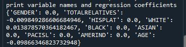
Lasso

Predictor variables and the Regression Coefficients

Predictor variables with regression coefficients equal to zero means that the coefficients for those variables had shrunk to zero after applying the LASSO regression penalty, and were subsequently removed from the model. So the results show that of the 9 variables, 3 were chosen in the final model. All the variables were standardized on the same scale so we can also use the size of the regression coefficients to tell us which predictors are the strongest predictors of drinking status. For example, White ethnicity had the largest regression coefficient and was most strongly associated with drinking status. Age and total number of relatives with drinking problems were negatively associated with drinking status.

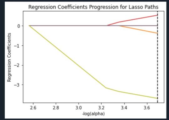
Regression Coefficients Progression Plot

This plot shows the relative importance of the predictor variable selected at any step of the selection process, how the regression coefficients changed with the addition of a new predictor at each step, and the steps at which each variable entered the new model. Age was entered first, it is the largest negative coefficient, then White ethnicity (the largest positive coefficient), and then Total Relatives (a negative coefficient).

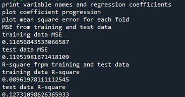
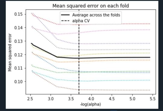
Mean Square Error Plot

The Mean Square Error plot shows the change in mean square error for the change in the penalty parameter alpha at each step in the selection process. The plot shows that there is variability across the individual cross-validation folds in the training data set, but the change in the mean square error as variables are added to the model follows the same pattern for each fold. Initially it decreases, and then levels off to a point a which adding more predictors doesn’t lead to much reduction in the mean square error.

Mean Square Error for Training and Test Data

Training: 0.11656843533066587

Test: 0.11951981671418109

The test mean square error was very close to the training mean square error, suggesting that prediction accuracy was pretty stable across the two data sets.

R-Square from Training and Test Data

Training: 0.08961978111112545

Test: 0.12731098626365933

The R-Square values were 0.09 and 0.13, indicating that the selected model explained 9% and 13% of the variance in drinking status for the training and the test sets, respectively. This suggests that I should think about adding more explanatory variables but I must be careful and watch for an increase in variance and bias.

Python Code

from pandas import Series, DataFrame import pandas import numpy import os import matplotlib.pylab as plt from sklearn.model_selection import train_test_split from sklearn.linear_model import LassoLarsCV

os.environ['PATH'] = os.environ['PATH']+';'+os.environ['CONDA_PREFIX']+r"\Library\bin\graphviz"

data = pandas.read_csv('nesarc_pds.csv', low_memory=False)

## Machine learning week 3 addition## #upper-case all DataFrame column names data.columns = map(str.upper, data.columns) ## Machine learning week 3 addition##

#setting variables you will be working with to numeric data['IDNUM'] =pandas.to_numeric(data['IDNUM'], errors='coerce') data['AGE'] =pandas.to_numeric(data['AGE'], errors='coerce') data['SEX'] = pandas.to_numeric(data['SEX'], errors='coerce') data['S2AQ16A'] =pandas.to_numeric(data['S2AQ16A'], errors='coerce') data['S2BQ2D'] =pandas.to_numeric(data['S2BQ2D'], errors='coerce') data['S2DQ1'] =pandas.to_numeric(data['S2DQ1'], errors='coerce') data['S2DQ2'] =pandas.to_numeric(data['S2DQ2'], errors='coerce') data['S2DQ11'] =pandas.to_numeric(data['S2DQ11'], errors='coerce') data['S2DQ12'] =pandas.to_numeric(data['S2DQ12'], errors='coerce') data['S2DQ13A'] =pandas.to_numeric(data['S2DQ13A'], errors='coerce') data['S2DQ13B'] =pandas.to_numeric(data['S2DQ13B'], errors='coerce') data['S2DQ7C1'] =pandas.to_numeric(data['S2DQ7C1'], errors='coerce') data['S2DQ7C2'] =pandas.to_numeric(data['S2DQ7C2'], errors='coerce') data['S2DQ8C1'] =pandas.to_numeric(data['S2DQ8C1'], errors='coerce') data['S2DQ8C2'] =pandas.to_numeric(data['S2DQ8C2'], errors='coerce') data['S2DQ9C1'] =pandas.to_numeric(data['S2DQ9C1'], errors='coerce') data['S2DQ9C2'] =pandas.to_numeric(data['S2DQ9C2'], errors='coerce') data['S2DQ10C1'] =pandas.to_numeric(data['S2DQ10C1'], errors='coerce') data['S2DQ10C2'] =pandas.to_numeric(data['S2DQ10C2'], errors='coerce') data['S2BQ3A'] =pandas.to_numeric(data['S2BQ3A'], errors='coerce')

###### WEEK 4 ADDITIONS #####

#hispanic or latino data['S1Q1C'] =pandas.to_numeric(data['S1Q1C'], errors='coerce')

#american indian or alaskan native data['S1Q1D1'] =pandas.to_numeric(data['S1Q1D1'], errors='coerce')

#black or african american data['S1Q1D3'] =pandas.to_numeric(data['S1Q1D3'], errors='coerce')

#asian data['S1Q1D2'] =pandas.to_numeric(data['S1Q1D2'], errors='coerce')

#native hawaiian or pacific islander data['S1Q1D4'] =pandas.to_numeric(data['S1Q1D4'], errors='coerce')

#white data['S1Q1D5'] =pandas.to_numeric(data['S1Q1D5'], errors='coerce')

#consumer data['CONSUMER'] =pandas.to_numeric(data['CONSUMER'], errors='coerce')

data_clean = data.dropna()

data_clean.dtypes data_clean.describe()

sub1=data_clean[['IDNUM', 'AGE', 'SEX', 'S2AQ16A', 'S2BQ2D', 'S2BQ3A', 'S2DQ1', 'S2DQ2', 'S2DQ11', 'S2DQ12', 'S2DQ13A', 'S2DQ13B', 'S2DQ7C1', 'S2DQ7C2', 'S2DQ8C1', 'S2DQ8C2', 'S2DQ9C1', 'S2DQ9C2', 'S2DQ10C1', 'S2DQ10C2', 'S1Q1C', 'S1Q1D1', 'S1Q1D2', 'S1Q1D3', 'S1Q1D4', 'S1Q1D5', 'CONSUMER']]

sub2=sub1.copy()

#setting variables you will be working with to numeric cols = sub2.columns sub2[cols] = sub2[cols].apply(pandas.to_numeric, errors='coerce')

#subset data to people age 6 to 80 who have become alcohol dependent sub3=sub2[(sub2['S2AQ16A']>=5) & (sub2['S2AQ16A']<=83)]

#make a copy of my new subsetted data sub4 = sub3.copy()

#Explanatory Variables for Relatives #recode - nos set to zero recode1 = {1: 1, 2: 0, 3: 0}

sub4['DAD']=sub4['S2DQ1'].map(recode1) sub4['MOM']=sub4['S2DQ2'].map(recode1) sub4['PATGRANDDAD']=sub4['S2DQ11'].map(recode1) sub4['PATGRANDMOM']=sub4['S2DQ12'].map(recode1) sub4['MATGRANDDAD']=sub4['S2DQ13A'].map(recode1) sub4['MATGRANDMOM']=sub4['S2DQ13B'].map(recode1) sub4['PATBROTHER']=sub4['S2DQ7C2'].map(recode1) sub4['PATSISTER']=sub4['S2DQ8C2'].map(recode1) sub4['MATBROTHER']=sub4['S2DQ9C2'].map(recode1) sub4['MATSISTER']=sub4['S2DQ10C2'].map(recode1)

#### WEEK 4 ADDITIONS #### sub4['HISPLAT']=sub4['S1Q1C'].map(recode1) sub4['AMERIND']=sub4['S1Q1D1'].map(recode1) sub4['ASIAN']=sub4['S1Q1D2'].map(recode1) sub4['BLACK']=sub4['S1Q1D3'].map(recode1) sub4['PACISL']=sub4['S1Q1D4'].map(recode1) sub4['WHITE']=sub4['S1Q1D5'].map(recode1) sub4['DRINKSTAT']=sub4['CONSUMER'].map(recode1) sub4['GENDER']=sub4['SEX'].map(recode1) #### END WEEK 4 ADDITIONS ####

#Replacing unknowns with NAN sub4['DAD']=sub4['DAD'].replace(9, numpy.nan) sub4['MOM']=sub4['MOM'].replace(9, numpy.nan) sub4['PATGRANDDAD']=sub4['PATGRANDDAD'].replace(9, numpy.nan) sub4['PATGRANDMOM']=sub4['PATGRANDMOM'].replace(9, numpy.nan) sub4['MATGRANDDAD']=sub4['MATGRANDDAD'].replace(9, numpy.nan) sub4['MATGRANDMOM']=sub4['MATGRANDMOM'].replace(9, numpy.nan) sub4['PATBROTHER']=sub4['PATBROTHER'].replace(9, numpy.nan) sub4['PATSISTER']=sub4['PATSISTER'].replace(9, numpy.nan) sub4['MATBROTHER']=sub4['MATBROTHER'].replace(9, numpy.nan) sub4['MATSISTER']=sub4['MATSISTER'].replace(9, numpy.nan) sub4['S2DQ7C1']=sub4['S2DQ7C1'].replace(99, numpy.nan) sub4['S2DQ8C1']=sub4['S2DQ8C1'].replace(99, numpy.nan) sub4['S2DQ9C1']=sub4['S2DQ9C1'].replace(99, numpy.nan) sub4['S2DQ10C1']=sub4['S2DQ10C1'].replace(99, numpy.nan) sub4['S2AQ16A']=sub4['S2AQ16A'].replace(99, numpy.nan) sub4['S2BQ2D']=sub4['S2BQ2D'].replace(99, numpy.nan) sub4['S2BQ3A']=sub4['S2BQ3A'].replace(99, numpy.nan)

#add parents togetheR sub4['IFPARENTS'] = sub4['DAD'] + sub4['MOM']

#add grandparents together sub4['IFGRANDPARENTS'] = sub4['PATGRANDDAD'] + sub4['PATGRANDMOM'] + sub4['MATGRANDDAD'] + sub4['MATGRANDMOM']

#add IF aunts and uncles together sub4['IFUNCLEAUNT'] = sub4['PATBROTHER'] + sub4['PATSISTER'] + sub4['MATBROTHER'] + sub4['MATSISTER']

#add SUM uncle and aunts together sub4['SUMUNCLEAUNT'] = sub4['S2DQ7C1'] + sub4['S2DQ8C1'] + sub4['S2DQ9C1'] + sub4['S2DQ10C1']

#add relatives together sub4['SUMRELATIVES'] = sub4['IFPARENTS'] + sub4['IFGRANDPARENTS'] + sub4['SUMUNCLEAUNT']

def TOTALRELATIVES (row): if row['SUMRELATIVES'] == 0 : return 0 elif row['SUMRELATIVES'] >= 1 : return 1

sub4['TOTALRELATIVES'] = sub4.apply (lambda row: TOTALRELATIVES (row), axis=1)

sub4_clean = sub4.dropna()

sub4_clean.dtypes sub4_clean.describe()

###Machine Learning week 3 additions##

#select predictor variables and target variable as separate data sets

predvar = sub4_clean[['GENDER','TOTALRELATIVES', 'HISPLAT', 'WHITE', 'BLACK', 'ASIAN', 'PACISL', 'AMERIND', 'AGE']]

target = sub4_clean.DRINKSTAT

# standardize predictors to have mean=0 and sd=1 predictors=predvar.copy() from sklearn import preprocessing

predictors['GENDER']=preprocessing.scale(predictors['GENDER'].astype('float64')) predictors['TOTALRELATIVES']=preprocessing.scale(predictors['TOTALRELATIVES'].astype('float64')) predictors['HISPLAT']=preprocessing.scale(predictors['HISPLAT'].astype('float64')) predictors['WHITE']=preprocessing.scale(predictors['WHITE'].astype('float64')) predictors['BLACK']=preprocessing.scale(predictors['BLACK'].astype('float64')) predictors['ASIAN']=preprocessing.scale(predictors['ASIAN'].astype('float64')) predictors['PACISL']=preprocessing.scale(predictors['PACISL'].astype('float64')) predictors['AMERIND']=preprocessing.scale(predictors['AMERIND'].astype('float64')) predictors['AGE']=preprocessing.scale(predictors['AGE'].astype('float64'))

# split data into train and test sets pred_train, pred_test, tar_train, tar_test = train_test_split(predictors, target, test_size=.3, random_state=123)

# specify the lasso regression model model=LassoLarsCV(cv=10, precompute=False).fit(pred_train,tar_train)

# print variable names and regression coefficients print("print variable names and regression coefficients") coef_dict = dict(zip(predictors.columns, model.coef_)) print(coef_dict)

# plot coefficient progression print("plot coefficient progression") m_log_alphas = -numpy.log10(model.alphas_) ax = plt.gca() plt.plot(m_log_alphas, model.coef_path_.T) plt.axvline(-numpy.log10(model.alpha_), linestyle='--', color='k', label='alpha CV') plt.ylabel('Regression Coefficients') plt.xlabel('-log(alpha)') plt.title('Regression Coefficients Progression for Lasso Paths')

# plot mean square error for each fold print("plot mean square error for each fold") m_log_alphascv = -numpy.log10(model.cv_alphas_) plt.figure() plt.plot(m_log_alphascv, model.cv_mse_path_, ':') plt.plot(m_log_alphascv, model.cv_mse_path_.mean(axis=-1), 'k', label='Average across the folds', linewidth=2) plt.axvline(-numpy.log10(model.alpha_), linestyle='--', color='k', label='alpha CV') plt.legend() plt.xlabel('-log(alpha)') plt.ylabel('Mean squared error') plt.title('Mean squared error on each fold')

# MSE from training and test data print("MSE from training and test data") from sklearn.metrics import mean_squared_error train_error = mean_squared_error(tar_train, model.predict(pred_train)) test_error = mean_squared_error(tar_test, model.predict(pred_test)) print ('training data MSE') print(train_error) print ('test data MSE') print(test_error)

# R-square from training and test data print("R-square frpm training and test data") rsquared_train=model.score(pred_train,tar_train) rsquared_test=model.score(pred_test,tar_test) print ('training data R-square') print(rsquared_train) print ('test data R-square') print(rsquared_test)

1 note · View note

jyotikharade · 5 years ago

Text

Decision Tree

Machine Learning(ML):

Classification Tree:

CODING:

# coding: utf-8

“’

Decision tree to predict survival on the TtTanic

”’

get_ipython().magic(‘matplotlib inline’)

from pandas import Series, DataFrame

import pandas as pd

import numpy as np

import os

import matplotlib.pylab as plt

from sklearn.cross_validation import train_test_split

from sklearn.tree import DecisionTreeClassifier

from sklearn.metrics import classification_report

import sklearn.metrics

titanic = pd.read_csv('train.csv’)

print(titanic.describe())

print(titanic.head(5))

print(titanic.info())

# simplify Age

def catAge (row):

if row['Age’] <= 8 :

return 0

elif row['Age’] <= 16 :

return 1

elif row['Age’] <= 60 :

return 2

else:

return 2

# create categorical varioble for sex 1 = female, 0 = male

titanic['Gender’] = titanic['Sex’].map( {'female’: 1, 'male’: 0} ).astype(int)

# create age categories either 1 = Adult or 0 = child

titanic['AgeCat’] = titanic.apply(lambda row:catAge(row), axis = 1)

print(titanic.dtypes)

# get a clean subset

sub = titanic[['PassengerId’, 'Gender’,'Pclass’, 'AgeCat’,'SibSp’, 'Survived’]].dropna()

sub['Gender’] = sub['Gender’].astype('category’)

sub['AgeCat’] = sub['AgeCat’].astype('category’)

sub['Pclass’] = sub['Pclass’].astype('category’)

print(sub.info())

# Split the data

predictors = sub[['Gender’,'Pclass’, 'AgeCat’,'SibSp’]]

targets = sub['Survived’]

pred_train, pred_test, tar_train, tar_test = train_test_split(predictors, targets, test_size=.4)

print(pred_train.shape, ’\n’,

pred_test.shape,’\n’,

tar_train.shape,’\n’,

tar_test.shape)

#Build model on training data

classifier=DecisionTreeClassifier()

classifier=classifier.fit(pred_train,tar_train)

predictions=classifier.predict(pred_test)

print(’\nConfusion Matrix’)

print(sklearn.metrics.confusion_matrix(tar_test,predictions))

print('Accuracy Score’)

print(sklearn.metrics.accuracy_score(tar_test, predictions))

#Displaying the decision tree

from sklearn import tree

#from StringIO import StringIO

from io import StringIO

#from StringIO import StringIO

from IPython.display import Image

out = StringIO()

tree.export_graphviz(classifier, out_file=out, feature_names = ['Gender’, 'Pclass’,'AgeCat’,'SibSp’],filled = True)

import pydotplus

graph=pydotplus.graph_from_dot_data(out.getvalue())

Image(graph.create_png())

# Split the data

predictors = sub[['Gender’,'Pclass’, 'AgeCat’]]

targets = sub['Survived’]

pred_train, pred_test, tar_train, tar_test = train_test_split(predictors, targets, test_size=.4)

print(pred_train.shape, ’\n’,

pred_test.shape,’\n’,

tar_train.shape,’\n’,

tar_test.shape)

#Build model on training data

classifier=DecisionTreeClassifier()

classifier=classifier.fit(pred_train,tar_train)

# Make prediction on the test data

predictions=classifier.predict(pred_test)

# Confusion Matrix

print('Confusion Matrix’)

print(sklearn.metrics.confusion_matrix(tar_test,predictions))

#Accuracy

print('Accuracy Score’)

print(sklearn.metrics.accuracy_score(tar_test, predictions))

# Show the tree

out = StringIO()

tree.export_graphviz(classifier, out_file=out, feature_names = ['Gender’,'Pclass’, 'AgeCat’],filled = True)

# Save tree as png file

graph=pydotplus.graph_from_dot_data(out.getvalue())

Image(graph.create_png())

print(pred_train.describe())

# Observe various features of the traning data

print(titanic.Gender.sum())

print(titanic.Gender.count())

print(titanic.Gender.sum()/titanic.Gender.count())

# Table of survival Vs Gender

pd.crosstab(titanic.Sex,titanic.Survived)

1 note

RECENTLY LIKED

understands

compulsive

197,804 notes

1 note · View note

akashkudale · 5 years ago

Text

Decision Tree

Machine Learning(ML):

Classification Tree:

CODING:

# coding: utf-8

“’

Decision tree to predict survival on the TtTanic

”’

get_ipython().magic('matplotlib inline’)

from pandas import Series, DataFrame

import pandas as pd

import numpy as np

import os

import matplotlib.pylab as plt

from sklearn.cross_validation import train_test_split

from sklearn.tree import DecisionTreeClassifier

from sklearn.metrics import classification_report

import sklearn.metrics

titanic = pd.read_csv('train.csv’)

print(titanic.describe())

print(titanic.head(5))

print(titanic.info())

# simplify Age

def catAge (row):

if row['Age’] <= 8 :

return 0

elif row['Age’] <= 16 :

return 1

elif row['Age’] <= 60 :

return 2

else:

return 2

# create categorical varioble for sex 1 = female, 0 = male

titanic['Gender’] = titanic['Sex’].map( {'female’: 1, 'male’: 0} ).astype(int)

# create age categories either 1 = Adult or 0 = child

titanic['AgeCat’] = titanic.apply(lambda row:catAge(row), axis = 1)

print(titanic.dtypes)

# get a clean subset

sub = titanic[['PassengerId’, 'Gender’,'Pclass’, 'AgeCat’,'SibSp’, 'Survived’]].dropna()

sub['Gender’] = sub['Gender’].astype('category’)

sub['AgeCat’] = sub['AgeCat’].astype('category’)

sub['Pclass’] = sub['Pclass’].astype('category’)

print(sub.info())

# Split the data

predictors = sub[['Gender’,'Pclass’, 'AgeCat’,'SibSp’]]

targets = sub['Survived’]

pred_train, pred_test, tar_train, tar_test = train_test_split(predictors, targets, test_size=.4)

print(pred_train.shape, ’\n’,

pred_test.shape,’\n’,

tar_train.shape,’\n’,

tar_test.shape)

#Build model on training data

classifier=DecisionTreeClassifier()

classifier=classifier.fit(pred_train,tar_train)

predictions=classifier.predict(pred_test)

print(’\nConfusion Matrix’)

print(sklearn.metrics.confusion_matrix(tar_test,predictions))

print('Accuracy Score’)

print(sklearn.metrics.accuracy_score(tar_test, predictions))

#Displaying the decision tree

from sklearn import tree

#from StringIO import StringIO

from io import StringIO

#from StringIO import StringIO

from IPython.display import Image

out = StringIO()

tree.export_graphviz(classifier, out_file=out, feature_names = ['Gender’, 'Pclass’,'AgeCat’,'SibSp’],filled = True)

import pydotplus

graph=pydotplus.graph_from_dot_data(out.getvalue())

Image(graph.create_png())

# Split the data

predictors = sub[['Gender’,'Pclass’, 'AgeCat’]]

targets = sub['Survived’]

pred_train, pred_test, tar_train, tar_test = train_test_split(predictors, targets, test_size=.4)

print(pred_train.shape, ’\n’,

pred_test.shape,’\n’,

tar_train.shape,’\n’,

tar_test.shape)

#Build model on training data

classifier=DecisionTreeClassifier()

classifier=classifier.fit(pred_train,tar_train)

# Make prediction on the test data

predictions=classifier.predict(pred_test)

# Confusion Matrix

print('Confusion Matrix’)

print(sklearn.metrics.confusion_matrix(tar_test,predictions))

#Accuracy

print('Accuracy Score’)

print(sklearn.metrics.accuracy_score(tar_test, predictions))

# Show the tree

out = StringIO()

tree.export_graphviz(classifier, out_file=out, feature_names = ['Gender’,'Pclass’, 'AgeCat’],filled = True)

# Save tree as png file

graph=pydotplus.graph_from_dot_data(out.getvalue())

Image(graph.create_png())

print(pred_train.describe())

# Observe various features of the traning data

print(titanic.Gender.sum())

print(titanic.Gender.count())

print(titanic.Gender.sum()/titanic.Gender.count())

# Table of survival Vs Gender

pd.crosstab(titanic.Sex,titanic.Survived)

1 note · View note

govindhtech · 11 months ago

Text

Exploring BigQuery DataFrames and LLMs data production

Data processing and machine learning operations have been difficult to separate in big data analytics. Data engineers used Apache Spark for large-scale data processing in BigQuery, while data scientists used pandas and scikit-learn for machine learning. This disconnected approach caused inefficiencies, data duplication, and data insight delays.

At the same time, AI success depends on massive data. Thus, any firm must generate and handle synthetic data, which replicates real-world data. Algorithmically modelling production datasets or training ML algorithms like generative AI generate synthetic data. This synthetic data can simulate operational or production data for ML model training or mathematical model evaluation.

BigQuery DataFrames Solutions

BigQuery DataFrames unites data processing with machine learning on a scalable, cost-effective platform. This helps organizations expedite data-driven initiatives, boost teamwork, and maximize data potential. BigQuery DataFrames is an open-source Python package with pandas-like DataFrames and scikit-learn-like ML libraries for huge data.

It runs on BigQuery and Google Cloud storage and compute. Integrating with Google Cloud Functions allows compute extensibility, while Vertex AI delivers generative AI capabilities, including state-of-the-art models. BigQuey DataFrames can be utilized to build scalable AI applications due to their versatility.

BigQuery DataFrames lets you generate artificial data at scale and avoids concerns with transporting data beyond your ecosystem or using third-party solutions. When handling sensitive personal data, synthetic data protects privacy. It permits dataset sharing and collaboration without disclosing personal details.

Google Cloud can also apply analytical models in production. Testing and validation are safe with synthetic data. Simulate edge cases, outliers, and uncommon events that may not be in your dataset. Synthetic data also lets you model data warehouse schema or ETL process modifications before making them, eliminating costly errors and downtime.

Synthetic data generation with BigQuery DataFrames

Many applications require synthetic data generation:

Real data generation is costly and slow.

Unlike synthetic data, original data is governed by strict laws, restrictions, and oversight.

Simulations require larger data.

What is a data schema

Data schema

Let’s use BigQuery DataFrames and LLMs to produce synthetic data in BigQuery. Two primary stages and several substages comprise this process:

Code creation

Set the Schema and instruct LLM.

The user knows the expected data schema.

They understand data-generating programmes at a high degree.

They intend to build small-scale data generation code in a natural language (NL) prompt.

Add hints to the prompt to help LLM generate correct code.

Send LLM prompt and get code.

Executing code

Run the code as a remote function at the specified scale.

Post-process Data to desired form.

Library setup and initialization.

Start by installing, importing, and initializing BigQuery DataFrames.

Start with user-specified schema to generate synthetic data.

Provide high-level schema.

Consider generating demographic data with name, age, and gender using gender-inclusive Latin American names. The prompt states our aim. They also provide other information to help the LLM generate the proper code:

Use Faker, a popular Python fake data module, as a foundation.

Pandas DataFrame holds lesser data.

Generate code with LLM.

Note that they will produce code to construct 100 rows of the intended data before scaling it.

Run code

They gave LLMs all the guidance they needed and described the dataset structure in the preceding stage. The code is verified and executed here. This process is crucial since it involves humans and validates output.

Local code verification with a tiny sample

The prior stage’s code appears fine.

They would return to the prompt and update it and repeat the procedures if the created code hadn’t ran or Google wanted to fine-tune the data distribution.

The LLM prompt might include the created code and the issue to repair.

Deploy code as remote function

The data matches what they wanted, so Google may deploy the app as a remote function. Remote functions offer scalar transformation, thus Google can utilize an indicator (in this case integer) input and make a string output, which is the code’s serialized dataframe in json. Google Cloud must additionally mention external package dependencies, such as faker and pandas.

Scale data generation

Create one million synthetic data rows. An indicator dataframe with 1M/100 = 10K indicator rows can be initialized since our created code generates 100 rows every run. They can use the remote function to generate 100 synthetic data rows each indication row.

Flatten JSON

Each item in df[“json_data”] is a 100-record json serialized array. Use direct SQL to flatten that into one record per row.

The result_df DataFrame contains one million synthetic data rows suitable for usage or saving in a BigQuery database (using the to_gbq method). BigQuery, Vertex AI, Cloud Functions, Cloud Run, Cloud Build, and Artefact Registry fees are involved. BigQuery DataFrames pricing details. BigQuery jobs utilized ~276K slot milliseconds and processed ~62MB bytes.

Creating synthetic data from a table structure

A schema can generate synthetic data, as seen in the preceding step. Synthetic data for an existing table is possible. You may be copying the production dataset for development. The goal is to ensure data distribution and schema similarity. This requires creating the LLM prompt from the table’s column names, types, and descriptions. The prompt could also include data profiling metrics derived from the table’s data, such as:

Any numeric column distribution. DataFrame.describe returns column statistics.

Any suggestions for string or date/time column data format. Use DataFrame.sample or Series.sample.

Any tips on unique categorical column values. You can use Series.unique.

Existing dimension table fact table generation

They could create a synthetic fact table for a dimension table and join it back. If your usersTable has schema (userId, userName, age, gender), you can construct a transactionsTable with schema (userId, transactionDate, transactionAmount) where userId is the key relationship. To accomplish this, take these steps:

Create LLM prompt to produce schema data (transactionDate, transactionAmount).

(Optional) In the prompt, tell the algorithm to generate a random number of rows between 0 and 100 instead of 100 to give fact data a more natural distribution. You need adjust batch_size to 50 (assuming symmetrical distribution). Due to unpredictability, the final data may differ from the desired_num_rows.

Replace the schema range with userId from the usersTable to initialise the indicator dataframe.

As with the given schema, run the LLM-generated code remote function on the indicator dataframe.

Select userId and (transactionDate, transactionAmount) in final result.

Conclusions and resources

This example used BigQuery DataFrames to generate synthetic data, essential in today’s AI world. Synthetic data is a good alternative for training machine learning models and testing systems due to data privacy concerns and the necessity for big datasets. BigQuery DataFrames integrates easily with your data warehouse, Vertex AI, and the advanced Gemini model. This lets you generate data in your data warehouse without third-party solutions or data transfer.

Google Cloud demonstrated BigQuery DataFrames and LLMs synthetic data generation step-by-step. This involves:

Set the data format and use natural language prompts to tell the LLM to generate code.

Code execution: Scaling the code as a remote function to generate massive amounts of synthetic data.

Get the full Colab Enterprise notebook source code here.

Google also offered three ways to use their technique to demonstrate its versatility:

From user-specified schema, generate data: Ideal for pricey data production or rigorous governance.

Generate data from a table schema: Useful for production-like development datasets.

Create a dimension table fact table: Allows entity-linked synthetic transactional data creation.

BigQuery DataFrames and LLMs may easily generate synthetic data, alleviating data privacy concerns and boosting AI development.

Read more on Govindhtech.com

#bigquery #bigquerydataframes #dataframes #machinelearning #govindhtech #vertexai #news #technews #technology #technologynews #technologytrends #googlecloud #dataschema

0 notes

iamcalledabhi-blog · 5 years ago

Text

Decision Tree

Machine Learning(ML):

Classification Tree:

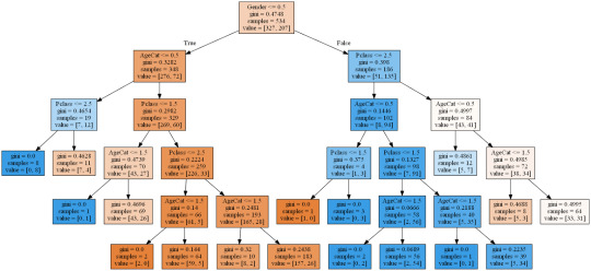
CODING:

# coding: utf-8

“’

Decision tree to predict survival on the TtTanic

”’

get_ipython().magic('matplotlib inline’)

from pandas import Series, DataFrame

import pandas as pd

import numpy as np

import os

import matplotlib.pylab as plt

from sklearn.cross_validation import train_test_split

from sklearn.tree import DecisionTreeClassifier

from sklearn.metrics import classification_report

import sklearn.metrics

titanic = pd.read_csv('train.csv’)

print(titanic.describe())

print(titanic.head(5))

print(titanic.info())

# simplify Age

def catAge (row):

if row['Age’] <= 8 :

return 0

elif row['Age’] <= 16 :

return 1

elif row['Age’] <= 60 :

return 2

else:

return 2

# create categorical varioble for sex 1 = female, 0 = male

titanic['Gender’] = titanic['Sex’].map( {'female’: 1, 'male’: 0} ).astype(int)

# create age categories either 1 = Adult or 0 = child

titanic['AgeCat’] = titanic.apply(lambda row:catAge(row), axis = 1)

print(titanic.dtypes)

# get a clean subset

sub = titanic[['PassengerId’, 'Gender’,'Pclass’, 'AgeCat’,'SibSp’, 'Survived’]].dropna()

sub['Gender’] = sub['Gender’].astype('category’)

sub['AgeCat’] = sub['AgeCat’].astype('category’)

sub['Pclass’] = sub['Pclass’].astype('category’)

print(sub.info())

# Split the data

predictors = sub[['Gender’,'Pclass’, 'AgeCat’,'SibSp’]]

targets = sub['Survived’]

pred_train, pred_test, tar_train, tar_test = train_test_split(predictors, targets, test_size=.4)

print(pred_train.shape, ’\n’,

pred_test.shape,’\n’,

tar_train.shape,’\n’,

tar_test.shape)

#Build model on training data

classifier=DecisionTreeClassifier()

classifier=classifier.fit(pred_train,tar_train)

predictions=classifier.predict(pred_test)

print(’\nConfusion Matrix’)

print(sklearn.metrics.confusion_matrix(tar_test,predictions))

print('Accuracy Score’)

print(sklearn.metrics.accuracy_score(tar_test, predictions))

#Displaying the decision tree

from sklearn import tree

#from StringIO import StringIO

from io import StringIO

#from StringIO import StringIO

from IPython.display import Image

out = StringIO()

tree.export_graphviz(classifier, out_file=out, feature_names = ['Gender’, 'Pclass’,'AgeCat’,'SibSp’],filled = True)

import pydotplus

graph=pydotplus.graph_from_dot_data(out.getvalue())

Image(graph.create_png())

# Split the data

predictors = sub[['Gender’,'Pclass’, 'AgeCat’]]

targets = sub['Survived’]

pred_train, pred_test, tar_train, tar_test = train_test_split(predictors, targets, test_size=.4)

print(pred_train.shape, ’\n’,

pred_test.shape,’\n’,

tar_train.shape,’\n’,

tar_test.shape)

#Build model on training data

classifier=DecisionTreeClassifier()

classifier=classifier.fit(pred_train,tar_train)

# Make prediction on the test data

predictions=classifier.predict(pred_test)

# Confusion Matrix

print('Confusion Matrix’)

print(sklearn.metrics.confusion_matrix(tar_test,predictions))

#Accuracy

print('Accuracy Score’)

print(sklearn.metrics.accuracy_score(tar_test, predictions))

# Show the tree

out = StringIO()

tree.export_graphviz(classifier, out_file=out, feature_names = ['Gender’,'Pclass’, 'AgeCat’],filled = True)

# Save tree as png file

graph=pydotplus.graph_from_dot_data(out.getvalue())

Image(graph.create_png())

print(pred_train.describe())

# Observe various features of the traning data

print(titanic.Gender.sum())

print(titanic.Gender.count())

print(titanic.Gender.sum()/titanic.Gender.count())

# Table of survival Vs Gender

pd.crosstab(titanic.Sex,titanic.Survived)

1 note · View note

chieffurycollection · 2 years ago

Text

Chi Square of alcohol abuse and number of alcoholic parents

Code:

-- coding: utf-8 --

""" Created on Wed Jun 14 11:18:20 2023

@author: """ import pandas import numpy import matplotlib.pyplot as plt import statsmodels.formula.api as smf import statsmodels.stats.multicomp as multi

import scipy.stats import seaborn

print("start import") data = pandas.read_csv('nesarc_pds.csv', low_memory=False) print("import done")

upper-case all Dataframe column names --> unification

data.columns = map(str.upper, data.columns.values.ravel())

bug fix for display formats to avoid run time errors

pandas.set_option('display.float_format', lambda x:'%f'%x)

print (len(data)) #number of observations (rows)

print (len(data.columns)) # number of variables (columns)

checking the format of your variables

setting variables you will be working with to numeric

data['S2DQ1'] = pandas.to_numeric(data['S2DQ1']) #Blood/Natural Father data['S2DQ2'] = pandas.to_numeric(data['S2DQ2']) #Blood/Natural Mother data['S2BQ3A'] = pandas.to_numeric(data['S2BQ3A'], errors='coerce') #Age at data['S3CQ14A3'] = pandas.to_numeric(data['S3CQ14A3'], errors='coerce')

Blood/Natural Father was alcoholic

print("number blood/natural father was alcoholic")

0 = no; 1= yes; unknown = nan

data['S2DQ1'] = data['S2DQ1'].replace({2: 0, 9: numpy.nan}) c1 = data['S2DQ1'].value_counts(sort=False).sort_index()

print (c1)

print("percentage blood/natural father was alcoholic")

p1 = data['S2DQ1'].value_counts(sort=False, normalize=True).sort_index()

print (p1)

Blood/Natural Mother was alcoholic

print("number blood/natural mother was alcoholic")

0 = no; 1= yes; unknown = nan

data['S2DQ2'] = data['S2DQ2'].replace({2: 0, 9: numpy.nan}) c2 = data['S2DQ2'].value_counts(sort=False).sort_index()

print(c2)

print("percentage blood/natural mother was alcoholic")

p2 = data['S2DQ2'].value_counts(sort=False, normalize=True).sort_index()

print (p2)

Data Management: Number of parents with background of alcoholism is calculated

0 = no parents; 1 = at least 1 parent (maybe one answer missing); 2 = 2 parents; nan = 1 unknown and 1 zero or both unknown

print("number blood/natural parents was alcoholic")

data['Num_alcoholic_parents'] = numpy.where((data['S2DQ1'] == 1) & (data['S2DQ2'] == 1), 2, numpy.where((data['S2DQ1'] == 1) & (data['S2DQ2'] == 0), 1, numpy.where((data['S2DQ1'] == 0) & (data['S2DQ2'].isna()), numpy.nan, numpy.where((data['S2DQ1'] == 0) & (data['S2DQ2'].isna()), numpy.nan, numpy.where((data['S2DQ1'] == 0) & (data['S2DQ2'] == 0), 0, numpy.nan)))))

c5 = data['Num_alcoholic_parents'].value_counts(sort=False).sort_index()

print(c5)

print("percentage blood/natural parents was alcoholic")

p5 = data['Num_alcoholic_parents'].value_counts(sort=False, normalize=True).sort_index()

print (p5)

Data Management: Age at onset of alcohol abuse --> Age is irrelevant; number of people with or without alcohol abuse is calculated

1 = alcohol abuse; 0 = no alcohol abuse; nan = unknown

print("number alcohol abuse")

replace age with 1

data['S2BQ3A'] = data['S2BQ3A'].replace({5: 1, 6: 1, 7: 1, 8: 1, 9: 1, 10: 1, 11: 1, 12: 1, 13: 1, 14: 1, 15: 1, 16: 1, 17: 1, 18: 1, 19: 1, 20: 1, 21: 1, 22: 1, 23: 1, 24: 1, 25: 1, 26: 1, 27: 1, 28: 1, 29: 1, 30: 1, 31: 1, 32: 1, 33: 1, 34: 1, 35: 1, 36: 1, 37: 1, 38: 1, 39: 1, 40: 1, 41: 1, 42: 1, 43: 1, 44: 1, 45: 1, 46: 1, 47: 1, 48: 1, 49: 1, 50: 1, 51: 1, 52: 1, 53: 1, 54: 1, 55: 1, 56: 1, 57: 1, 58: 1, 59: 1, 60: 1, 61: 1, 62: 1, 63: 1, 64: 1, 65: 1, 66: 1, 67: 1, 68: 1, 69: 1, 70: 1, 71: 1, 72: 1, 73: 1, 74: 1, 75: 1, 76: 1, 77: 1, 78: 1, 79: 1, 80: 1, 81: 1, 82: 1, 83: 1, 84: 1, 85: 1, 86: 1, 87: 1})

replace nan with 2

data['S2BQ3A'].fillna(0, inplace=True)

replace 99 with nan

data['S2BQ3A'] = data['S2BQ3A'].replace({99: numpy.nan}) c3 = data['S2BQ3A'].value_counts().sort_index()

print(c3)

print("percentage alcohol abuse")

p3 = data['S2BQ3A'].value_counts(sort=False, normalize=True).sort_index()

print (p3)

ever used Drugs/medicine in higher amount or longer period

0 = no; 1 = yes; nan = unknown

print("number drugs/medicine abuse")

blanks are filled with 0 (no abuse)

data['S3CQ14A3'].fillna(0, inplace=True) data['S3CQ14A3'] = data['S3CQ14A3'].replace({2: 0, 9: numpy.nan}) c4 = data['S3CQ14A3'].value_counts(sort=False).sort_index()

print(c4)

print("percentage drugs/medicine abuse")

p4 = data['S3CQ14A3'].value_counts(sort=False, normalize=True).sort_index()

print (p4)

Alcohol abuse vs. alcoholic parents

Daten filtern und gruppieren

filtered_data = data[data['S2BQ3A'] == 1] grouped_data = filtered_data.groupby('Num_alcoholic_parents').size()

Kategorien und Summen extrahieren

categories = grouped_data.index counts = grouped_data.values

Prozentsatz berechnen

total_count = numpy.sum(counts) percentages = (counts / total_count) * 100

plt.figure(figsize=(8, 5))

plt.bar(categories, percentages)

plt.xlabel('Num_alcoholic_parents')

plt.ylabel('Häufigkeit alcohol abuse in %')

plt.title('Häufigkeitsverteilung von alcohol abuse vs. alcoholic parents')

plt.xticks(c5.index)

plt.show()

Drug abuse vs. alcoholic parents

Daten filtern und gruppieren

filtered_data = data[data['S3CQ14A3'] == 1] grouped_data = filtered_data.groupby('Num_alcoholic_parents').size()

Kategorien und Summen extrahieren

categories = grouped_data.index counts = grouped_data.values

Prozentsatz berechnen

total_count = numpy.sum(counts) percentages = (counts / total_count) * 100

plt.figure(figsize=(8, 5))

plt.bar(categories, percentages)

plt.xlabel('Num_alcoholic_parents')

plt.ylabel('Häufigkeit drug abuse in %')

plt.title('Häufigkeitsverteilung von drug abuse vs. alcoholic parents')

plt.xticks(c5.index)

plt.show()

_______________________________________F statistics__________________________

print('f statistics')

using ols function for calculating the F-statistic and associated p value

model1 = smf.ols(formula='S2BQ3A ~ C(Num_alcoholic_parents)', data=data) results1 = model1.fit()

print (results1.summary())

print(' ')

using ols function for calculating the F-statistic and associated p value

model1 = smf.ols(formula='S3CQ14A3 ~ C(Num_alcoholic_parents)', data=data) results1 = model1.fit()

print (results1.summary())

sub2 = data[['Num_alcoholic_parents', 'S2BQ3A']].dropna()

print ('means for number alcoholic parents by alcohol abuse')

m1= sub2.groupby('S2BQ3A').mean()

print (m1)

print ('standard deviations for number alcoholic parents by alcohol abuse')

sd1 = sub2.groupby('S2BQ3A').std()

print (sd1)

i will call it sub3

sub3 = data[['Num_alcoholic_parents', 'S3CQ14A3']].dropna()

model2 = smf.ols(formula='Num_alcoholic_parents ~ C(S3CQ14A3)', data=sub3).fit()

print (model2.summary())

print ('means for number alcoholic parents by drug abuse')

m2= sub3.groupby('S3CQ14A3').mean()

print (m2)

print ('standard deviations for number alcoholic parents by drug abuse')

sd2 = sub3.groupby('S3CQ14A3').std()

print (sd2)

mc1 = multi.MultiComparison(sub3['S3CQ14A3'], sub3['Num_alcoholic_parents']) res1 = mc1.tukeyhsd()

print(res1.summary())

_________________________________________Chi Square____________________________________

is the number of parents with history of alcoholism 'Num_alcoholic_parents' in correlation with the abuse of alcohol 'S2BQ3A'

print('////////////////////////////////////////////////////////////////////////////////////////////////////////')

variables to numeric

data['Num_alcoholic_parents'] = pandas.to_numeric(data['Num_alcoholic_parents'], errors='coerce') data['S2BQ3A'] = pandas.to_numeric(data['S2BQ3A'], errors='coerce')

subset data to all who have abused alcohol

sub1=data

make a copy of my new subsetted data

sub2 = sub1.copy()

recode missing values to python missing (NaN)

sub2['Num_alcoholic_parents']=sub2['Num_alcoholic_parents'].replace(9, numpy.nan)

sub2['S2BQ3A']=sub2['S2BQ3A'].replace(99, numpy.nan)

contingency table of observed counts

ct1=pandas.crosstab(sub2['S2BQ3A'], sub2['Num_alcoholic_parents']) print (ct1) print(' ')

column percentages

colsum=ct1.sum(axis=0) colpct=ct1/colsum print(colpct) print(' ')

chi-square

print ('chi-square value, p value, expected counts') cs1= scipy.stats.chi2_contingency(ct1) print (cs1) print(' ')

set variable types

sub2["Num_alcoholic_parents"] = sub2["Num_alcoholic_parents"].astype('category')

new code for setting variables to numeric:

sub2['S2BQ3A'] = pandas.to_numeric(sub2['S2BQ3A'], errors='coerce')

graph percent with alcoholic parents dependence within each number of alcoholic parents group

seaborn.catplot(x="Num_alcoholic_parents", y="S2BQ3A", data=sub2, kind="bar", ci=None) plt.xlabel('number of alcoholic parents') plt.ylabel('Proportion alcohol abuse')

print(' ') recode2 = {0: 0, 1: 1} sub2['COMP0v1']= sub2['Num_alcoholic_parents'].map(recode2)

contingency table of observed counts

ct2=pandas.crosstab(sub2['S2BQ3A'], sub2['COMP0v1']) print (ct2)

print(' ')

column percentages

colsum=ct2.sum(axis=0) colpct=ct2/colsum print(colpct)

print ('chi-square value, p value, expected counts') cs2= scipy.stats.chi2_contingency(ct2) print (cs2) print(' ')

print(' ') recode3 = {1: 1, 2: 2} sub2['COMP1v2']= sub2['Num_alcoholic_parents'].map(recode3)

contingency table of observed counts

ct3=pandas.crosstab(sub2['S2BQ3A'], sub2['COMP1v2']) print (ct3)

print(' ')

column percentages

colsum=ct3.sum(axis=0) colpct=ct3/colsum print(colpct)

print ('chi-square value, p value, expected counts') cs3= scipy.stats.chi2_contingency(ct3) print (cs3) print(' ')

print(' ') recode4 = {0: 0, 2: 2} sub2['COMP0v2']= sub2['Num_alcoholic_parents'].map(recode4)

contingency table of observed counts

ct4=pandas.crosstab(sub2['S2BQ3A'], sub2['COMP0v2']) print (ct4)

print(' ')

column percentages

colsum=ct4.sum(axis=0) colpct=ct4/colsum print(colpct)

print ('chi-square value, p value, expected counts') cs4= scipy.stats.chi2_contingency(ct4) print (cs4) print(' ')

___________________________________________________________________________________

Result:

The plot shows that the higher the number of alcoholic parents, the higher the probability of alcohol abuse.

the p value is super low, so a dependence is indicated. the chi square tests of the different numbers of alcoholic parents also show very low p values and show that there is a dependence between the variables:

0 notes

usmanshami-blog · 5 years ago

Text

Trying out AWS SageMaker Studio for a simple machine learning task

Overview

Let’s look at how to accomplish a simple machine learning task on

AWS SageMaker

We'll take a movie ratings dataset comprising of user ratings for different movies and the movie metadata. Based on these existing user ratings of different movies, we'll try to predict what the user's rating would be for a movie that they haven't rated yet.

The following two documents are the primary references used in creating this doc - so feel free to refer to them in case there are any issues.

[1] Build, Train, and Deploy a Machine Learning Model (https://aws.amazon.com/getting-started/hands-on/build-train-deploy-machine-learning-model-sagemaker/) [2] Machine Learning Project – Data Science Movie Recommendation System Project in R (https://data-flair.training/blogs/data-science-r-movie-recommendation/)

We'd be using the MovieLens data from GroupLens Research.

[3] MovieLens | GroupLens (https://grouplens.org/datasets/movielens/)

Steps

Log into the AWS console and select Amazon SageMaker from the services to be redirected to the SageMaker Dashboard.

Select Amazon SageMaker Studio from the navigation bar on the left and select quick start to start a new instance of Amazon SageMaker Studio. Consider leaving the default name as is, select "Create a new role" in execution role and specify the S3 buckets you'd be using (Leaving these defaults should be okay as well) and click "Create Role". Once the execution role has been created, click on “Submit” - this will create a new Amazon SageMaker instance.

Once the Amazon SageMaker Studio instance is created, click on Open Studio link to launch the Amazon SageMaker Studio IDE.

Create a new Jupyter notebook using the Data Science as the Kernel and the latest python (Python 3) notebook.

Import the python libraries we'd be using in this task - boto3 is the python library which is used for making AWS requests, sagemaker is the sagemaker library and urllib.request is the library to make url requests such as HTTP GET etc to download csv files stored on S3 and elsewhere. numpy is a scientific computing python library and pandas is a python data analysis library. After writing the following code in the Jupyter notebook cell, look for a play button in the controls bar on top - click it should run the currently active cell and execute its code.

import boto3, sagemaker, urllib.request from sagemaker import get_execution_role import numpy as np import pandas as pd from sagemaker.predictor import csv_serializer

Once the imports have been completed, lets add some standard code to create execution role, define region settings and initialize boto for the region and xgboost

# Define IAM role role = get_execution_role() prefix = 'sagemaker/movielens' containers = {'us-west-2': '433757028032.dkr.ecr.us-west-2.amazonaws.com/xgboost:latest', 'us-east-1': '811284229777.dkr.ecr.us-east-1.amazonaws.com/xgboost:latest', 'us-east-2': '825641698319.dkr.ecr.us-east-2.amazonaws.com/xgboost:latest', 'eu-west-1': '685385470294.dkr.ecr.eu-west-1.amazonaws.com/xgboost:latest'} # each region has its XGBoost container my_region = boto3.session.Session().region_name # set the region of the instance print("Success - the MySageMakerInstance is in the " + my_region + " region. You will use the " + containers[my_region] + " container for your SageMaker endpoint.")

Create an S3 bucket that will contain our dataset files as well as training, test data, the computed machine learning models and the results.

bucket_name = '<BUCKET_NAME_HERE>' s3 = boto3.resource('s3') try: if my_region == 'us-east-1': s3.create_bucket(Bucket=bucket_name) else: s3.create_bucket(Bucket=bucket_name, CreateBucketConfiguration={ 'LocationConstraint': my_region }) print('S3 bucket created successfully') except Exception as e: print('S3 error: ',e)

Once the bucket has been created, upload the movie lens data files to the bucket by using the S3 console UI. You'll need to download the zip from https://grouplens.org/datasets/movielens/, extract it on the local machine and then upload the extracted files on S3. We used the Small dataset which has 100,000 ratings applied to 9,000 movies by 600 users. Be sure to read the MovieLens README file to make sure you understand the conditions on the data usage.

After the files have been uploaded, add the following code to the notebook to download the csv files and convert them to pandas data format

try: urllib.request.urlretrieve ("https://{}.s3.{}.amazonaws.com/ratings.csv".format(bucket_name, my_region), "ratings.csv") print('Success: downloaded ratings.csv.') except Exception as e: print('Data load error: ',e) try: urllib.request.urlretrieve ("https://{}.s3.{}.amazonaws.com/movies.csv".format(bucket_name, my_region), "movies.csv") print('Success: downloaded ratings.csv.') except Exception as e: print('Data load error: ',e)

try: model_data = pd.read_csv('./ratings.csv') print('Success: Data loaded into dataframe.') except Exception as e: print('Data load error: ',e) try: movie_data = pd.read_csv('./movies.csv') print('Success: Data loaded into dataframe.') except Exception as e: print('Data load error: ',e)

Now we create training and test datasets from the ratings data by splitting 70-30% the data randomly

train_data, test_data = np.split(model_data.sample(frac=1, random_state=1729), [int(0.7 * len(model_data))]) print(train_data.shape, test_data.shape) print(train_data.info, test_data.info)

We will need to normalize the training and test datasets to include boolean genre membership columns for each genre. To do this, we first process the movie dataset to create a movie to list of its genres map. Once the map has been created, we iterate the ratings data and update each row with the boolean genre membership columns. The following code creates the movie genre maps

movie_id_genre_map=dict() for movie_row in movie_data.itertuples(): # print (movie_row) genres=movie_row[3].split('|') # print(movie_row[1]) if movie_row[1] in movie_id_genre_map: raise movie_id_genre_map[movie_row[1]] = genres

print(len(movie_id_genre_map))

We now normalize the training data as mentioned above. Note that the rating column which is the column we are trying to predict in this model (and would be classifying into different rating classes) needs to be the first column in the training dataset. Also note that we multiplied the rating with 2 to convert it from 0.5-5 range of 0.5 rating increments to the range of 1-10. This is necessary since the new integer rating value becomes the rating class for the model classification.

normalized_train_data = list() for tuple in train_data.itertuples(): userId = tuple[1] movieId = tuple[2] rating = tuple[3]/0.5 timestamp = tuple[4] curr_row_normalized=dict() curr_row_normalized['rating'] = rating curr_row_normalized['userId'] = userId curr_row_normalized['movieId'] = movieId curr_row_normalized['timestamp'] = timestamp curr_genres = {'Action': 0, 'Adventure': 0, 'Animation': 0, 'Children': 0, 'Comedy': 0, 'Crime': 0, 'Documentary': 0, 'Drama': 0, 'Fantasy': 0, 'Film-Noir': 0, 'Horror': 0, 'Musical': 0, 'Mystery': 0, 'Romance': 0, 'Sci-Fi': 0, 'Thriller': 0, 'War': 0, 'Western': 0 } curr_movie = movie_id_genre_map[movieId] for genre in curr_movie: curr_genres[genre]=1

curr_row_normalized.update(curr_genres) normalized_train_data.append(curr_row_normalized) #print(curr_row_normalized) #print(normalized_train_data)

print(len(normalized_train_data)) normalized_train_data_pd = pd.DataFrame(data=normalized_train_data) print(normalized_train_data_pd.columns)

We do the same for test data, with a small difference - we create two different normalized data arrays - one with the user's rating and one without the user's rating. The one without the user's rating would be used in ML predictions - and these predictions would then be compared with the array with user's ratings to determine the accuracy of the predictions.

normalized_test_data = list() normalized_test_data_array = list() for tuple in test_data.itertuples(): userId = tuple[1] movieId = tuple[2] rating = tuple[3]/0.5 timestamp = tuple[4] curr_array_row_normalized=dict() curr_row_normalized=dict() curr_row_normalized['rating'] = rating curr_row_normalized['userId'] = userId curr_array_row_normalized['userId'] = userId curr_row_normalized['movieId'] = movieId curr_array_row_normalized['movieId'] = movieId curr_row_normalized['timestamp'] = timestamp curr_array_row_normalized['timestamp'] = timestamp curr_genres = {'Action': 0, 'Adventure': 0, 'Animation': 0, 'Children': 0, 'Comedy': 0, 'Crime': 0, 'Documentary': 0, 'Drama': 0, 'Fantasy': 0, 'Film-Noir': 0, 'Horror': 0, 'Musical': 0, 'Mystery': 0, 'Romance': 0, 'Sci-Fi': 0, 'Thriller': 0, 'War': 0, 'Western': 0 } curr_movie = movie_id_genre_map[movieId] for genre in curr_movie: curr_genres[genre]=1

curr_row_normalized.update(curr_genres) curr_array_row_normalized.update(curr_genres) normalized_test_data.append(curr_row_normalized) normalized_test_data_array.append(curr_array_row_normalized) #print(curr_row_normalized) #print(normalized_test_data) print(len(normalized_test_data)) print(len(normalized_test_data_array)) normalized_test_data_pd = pd.DataFrame(data=normalized_test_data) print(normalized_test_data_pd.columns) normalized_test_data_array_pd = pd.DataFrame(data=normalized_test_data_array) print(normalized_test_data_array_pd.columns)

Now lets run the predictions

xgb_predictor.content_type = 'text/csv' xgb_predictor.serializer = csv_serializer predictions = xgb_predictor.predict(normalized_test_data_array_pd.values).decode('utf-8') predictions_array = np.fromstring(predictions[1:], sep=',') # and turn the prediction into an array print(predictions_array)

Now create a frequency histogram of the rating classes for the predictions array - pandas crosstab utility does the trick here

cm = pd.crosstab(index=normalized_test_data_pd['rating'], columns=np.round(predictions_array), rownames=['Observed'], colnames=['Predicted'])

Now compute the accuracy of the prediction - we define the following classes - zero distance i.e. the prediction was accurate, one distance i.e. the predicted score differed from the actual by 1, two distance i.e. the predicted score differed from the actual by 2 and remaining i.e. the predicted score differed from actual by > 2

zero_distance = 0 one_distance = 0 two_distance = 0 remaining = 0 total = 0 for tuple in cm.itertuples(): total += tuple[0] total += tuple[1] total += tuple[2] total += tuple[3] total += tuple[4] total += tuple[5] total += tuple[6] total += tuple[7] total += tuple[8] total += tuple[9] total += tuple[10]

actual = tuple[0] if actual == 1.0: zero_distance += tuple[1] one_distance += tuple[2] two_distance += tuple[3] remaining += tuple[4] remaining += tuple[5] remaining += tuple[6] remaining += tuple[7] remaining += tuple[8] remaining += tuple[9] remaining += tuple[10]

if actual == 2.0: zero_distance += tuple[2] one_distance += tuple[1] one_distance += tuple[3] two_distance += tuple[4] remaining += tuple[5] remaining += tuple[6] remaining += tuple[7] remaining += tuple[8] remaining += tuple[9] remaining += tuple[10]

if actual == 3.0: zero_distance += tuple[3] one_distance += tuple[2] one_distance += tuple[4] two_distance += tuple[1] two_distance += tuple[5] remaining += tuple[6] remaining += tuple[7] remaining += tuple[8] remaining += tuple[9] remaining += tuple[10]

if actual == 4.0: zero_distance += tuple[4] one_distance += tuple[3] one_distance += tuple[5] two_distance += tuple[2] two_distance += tuple[6] remaining += tuple[1] remaining += tuple[7] remaining += tuple[8] remaining += tuple[9] remaining += tuple[10]

if actual == 5.0: zero_distance += tuple[5] one_distance += tuple[4] one_distance += tuple[6] two_distance += tuple[3] two_distance += tuple[7] remaining += tuple[1] remaining += tuple[2] remaining += tuple[8] remaining += tuple[9] remaining += tuple[10]

if actual == 6.0: zero_distance += tuple[6] one_distance += tuple[5] one_distance += tuple[7] two_distance += tuple[4] two_distance += tuple[8] remaining += tuple[1] remaining += tuple[2] remaining += tuple[3] remaining += tuple[9] remaining += tuple[10]

if actual == 7.0: zero_distance += tuple[7] one_distance += tuple[6] one_distance += tuple[8] two_distance += tuple[5] two_distance += tuple[9] remaining += tuple[1] remaining += tuple[2] remaining += tuple[3] remaining += tuple[4] remaining += tuple[10]

if actual == 8.0: zero_distance += tuple[8] one_distance += tuple[7] one_distance += tuple[9] two_distance += tuple[6] two_distance += tuple[10] remaining += tuple[1] remaining += tuple[2] remaining += tuple[3] remaining += tuple[4] remaining += tuple[5]

if actual == 9.0: zero_distance += tuple[9] one_distance += tuple[8] one_distance += tuple[10] two_distance += tuple[7] remaining += tuple[1] remaining += tuple[2] remaining += tuple[3] remaining += tuple[4] remaining += tuple[5] remaining += tuple[6]

if actual == 10.0: zero_distance += tuple[10] one_distance += tuple[9] two_distance += tuple[8] remaining += tuple[1] remaining += tuple[2] remaining += tuple[3] remaining += tuple[4] remaining += tuple[5] remaining += tuple[6] remaining += tuple[7]

zero_distance_percent = 100*(zero_distance/total) one_distance_percent = 100*(one_distance/total) two_distance_percent = 100*(two_distance/total) remaining_percent = 100*(remaining/total) print("zero distance percentage: "+str(zero_distance_percent)) print("one distance percentage: "+str(one_distance_percent)) print("two distance percentage: "+str(two_distance_percent)) print("remaining distance percentage: "+str(remaining_percent))

The results show that our model was 100% accurate for 11.4% predictions, had a deviation of 1 for 47.64% predictions, deviation of 2 for 13.51% predictions and deviation of > 2 for the remaining 27.24%

zero distance percentage: 11.403445800430726 one distance percentage: 47.641780330222545 two distance percentage: 13.513998564249821 remaining distance percentage: 27.243359655419958

Now terminate the sagemaker instance and free the allocated resources.

sagemaker.Session().delete_endpoint(xgb_predictor.endpoint) bucket_to_delete = boto3.resource('s3').Bucket(bucket_name) bucket_to_delete.objects.all().delete()

#AWS SageMaker #AWS #machine learning #SageMaker

1 note · View note