#skew symmetric matrix | Explore Tumblr posts and blogs

sethiswiftlearn · 3 months ago

Text

youtube

Class 12 Math | Matrices and Determinants part 2 | JEE Mains, CUET Prep

Matrices and Determinants are fundamental topics in Class 12 Mathematics, playing a crucial role in algebra and real-world applications. Mastering these concepts is essential for students preparing for competitive exams like JEE Mains, CUET, and other entrance tests. In this session, we continue exploring Matrices and Determinants (Part 2) with a deep dive into advanced concepts, problem-solving techniques, and shortcuts to enhance your mathematical skills.

What You’ll Learn in This Session?

In this second part of Matrices and Determinants, we cover: ✔ Types of Matrices & Their Properties – Understanding singular and non-singular matrices, symmetric and skew-symmetric matrices, and orthogonal matrices. ✔ Elementary Operations & Inverse of a Matrix – Step-by-step method to compute the inverse of a matrix using elementary transformations and properties of matrix operations. ✔ Adjoint and Cofactor of a Matrix – Learn how to find the adjoint and use it to compute the inverse efficiently. ✔ Determinants & Their Applications – Mastery of determinant properties and how they apply to solving equations. ✔ Solving Linear Equations using Matrices – Application of matrices in solving system of linear equations using Cramer’s Rule and Matrix Inversion Method. ✔ Shortcut Techniques & Tricks – Learn time-saving strategies to tackle complex determinant and matrix problems in exams.

Why is This Session Important?

Matrices and Determinants are not just theoretical concepts; they have wide applications in physics, computer science, economics, and engineering. Understanding their properties and operations simplifies problems in linear algebra, calculus, and probability. This topic is also heavily weighted in JEE Mains, CUET, and CBSE Board Exams, making it vital for scoring well.

Who Should Watch This?

JEE Mains Aspirants – Get an edge with advanced problem-solving strategies.

CUET & Other Competitive Exam Candidates – Build a strong foundation for entrance exams.

Class 12 CBSE & State Board Students – Strengthen concepts and improve exam performance.

Anyone Seeking Concept Clarity – If you want to master Matrices and Determinants, this session is perfect for you!

How Will This Help You?

Conceptual Clarity – Develop a clear understanding of matrices, their types, and operations.

Stronger Problem-Solving Skills – Learn various techniques and tricks to solve complex determinant problems quickly.

Exam-Focused Approach – Solve previous years' JEE Mains, CUET, and CBSE board-level questions.

Step-by-Step Explanations – Get detailed solutions to frequently asked questions in competitive exams.

Watch Now & Strengthen Your Math Skills!

Don't miss this in-depth session on Matrices and Determinants (Part 2). Strengthen your concepts, learn effective shortcuts, and boost your problem-solving skills to ace JEE Mains, CUET, and board exams.

📌 Watch here 👉 https://youtu.be/

🔔 Subscribe for More Updates! Stay tuned for more quick revision sessions, concept explanations, and exam tricks to excel in mathematics.

#Youtube

0 notes

infoclimb · 5 years ago

Photo

A set of mn elements arranged in a rectangular arrangement along m rows and n columns enclosed by the brackets [ ] or ( ) is called m by n matrix. The order of a matrix is a number of rows and columns of the matrix. For more info, visit:: mustknowfacts

0 notes

engineeringmathgeek · 6 years ago

Link

#symmetric matrix #orthogonal matrix #skew-symmetric matrix

0 notes

data-monkey · 6 years ago

Text

AO3 stats project: correlations

Okay. Now for some really fun stuff: correlations between different categories of metadata (like, correlations between ratings and tags, character tags and genre tags, etc). And as with the previous post in this series, some of the content I discuss may not be strictly work-appropriate.

Thanks to @eloiserummaging for beta reading these posts; any remaining errors are my own. A Python notebook showing the code I used to make these plots can be found here.

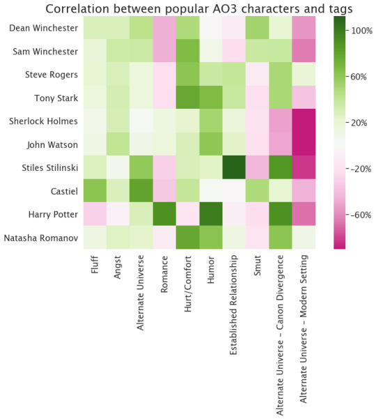
All right. We've got a list of top tags now. How do those tags relate to each other? That is, if I have a work labeled "Fluff", does that change how likely it is that that work will also be labeled "Angst"? I'm plotting, here, a matrix that answers that question directly. I can compute how often "Fluff" and "Angst" would appear together if they were just randomly assigned to all 4.3 million works that I collected metadata for. The blocks I'm showing below are colored by whether the actual number of times "Fluff" and "Angst" appear together is greater or lesser than that expectation. (We do it that way, instead of just counting the raw number of connections, because otherwise it looks like everything is correlated with "Fluff", just because there are a lot of works labeled "Fluff" in the data set.) If I pick two tags--say, "Fluff" on the bottom, and "Angst" on the left--I can follow them to where they intersect, and the color of that little block tells me about whether they're correlated. Things that are pink are less likely than you'd expect to appear together, while things that are green are more likely. The diagonal line is always that pale green-grey color because, by definition, "Romance" appears with "Romance" exactly as often as you'd expect, and the graph is symmetric across that diagonal line because it doesn't matter if we take "Fluff" then "Angst" or "Angst" then "Fluff."

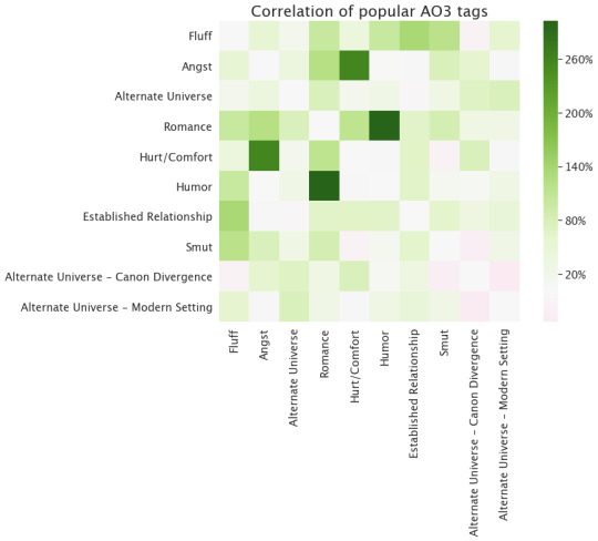
So one really interesting thing is that this plot is mostly green (so things are correlated). Not only do these tags appear a lot, but they appear together more than you’d expect, and even when they’re anti-correlated--that is, when being labeled one makes you less likely to be labeled another--it’s not by very much. The strongest correlation is between “Romance” and “Humor”, so I guess the rom com is alive and well! Angst and hurt/comfort also appear together a lot, which I suppose makes sense.

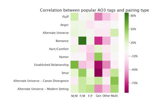
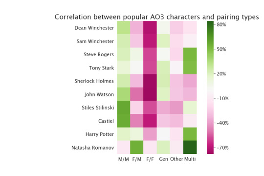
We can make correlation plots like this for other things. How about pairing types?

Per the AO3, “Multi” means “more than one kind of relationship, or a relationship with multiple partners”, and “Other” means “everything not covered by the other labels”. The structure of this is kind of interesting, too. Remember, pink means things are anti-correlated (appear together less often than expected) and green means they’re correlated (appear together MORE often than expected), so M/M is the Lone Ranger of pairing types, making all other pairing types less likely if it's included. Even more than Gen, which you’d expect to exclude other categories!

Now for the REALLY fun stuff: how do all of these things correlate with other things? Here's an obvious one: ratings vs tags. No more symmetry, because we're showing different things on the two axes.

Not too surprised by this: “Smut” has a really strong relationship with rating, because most works of erotica deserve the higher ratings. The other tags are much less correlated with rating; Fluff and Humor incline to lower ratings, Established Relationship to higher ratings, and the others are kind of in the middle.

Do ratings and tags correlate with pairing type?

Hmm. Interesting. Romance is way more likely to be F/M than you’d expect. (Do we not write as many M/M romances, or do we just call them something else? A couple of friends also pointed out to me that this might mean “romance” as in “the publication genre of romance” not as in “romantic plotlines generally”, which makes sense and would make them more M/F-heavy given publication trends.) Established relationship is very skewed to M/M. Gen anti-correlates with most of the tags you’d expect. Apparently only single-pairing romantic relationships can be fluffy. F/F is neither as funny nor as angsty as chance would indicate.

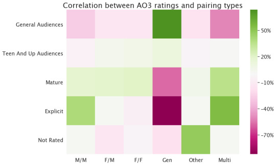
I think this pattern can be explained this way: Gen is way more likely to be a low rating, and the trend you see for most other things is just that we’re comparing to the average--if Gen is way more likely to be rated General Audiences than is typical, then the other pairing types have to be slightly less General Audiences than you’d expect to make up for it. (This argument doesn’t necessarily apply to the other correlations I was showing, because in those plots there are a bunch of tags I’m not showing and because non-ratings tags can appear together.)

How about the top relationship tags--do they correlate with anything?

Huh. Well, most of these ships have preferentially high ratings--I think that’s the same effect as in the rating and pairing correlation: things without a romantic/sexual relationship have lower ratings, so on average the works containing relationships will have a higher rating. That’s not universal--look at Magnus/Alec, for example--but it’s common. The other two obvious things here are 1) Dean/Sam really skews to high ratings, 2) apparently Harry/Louis fans reject the rating system.

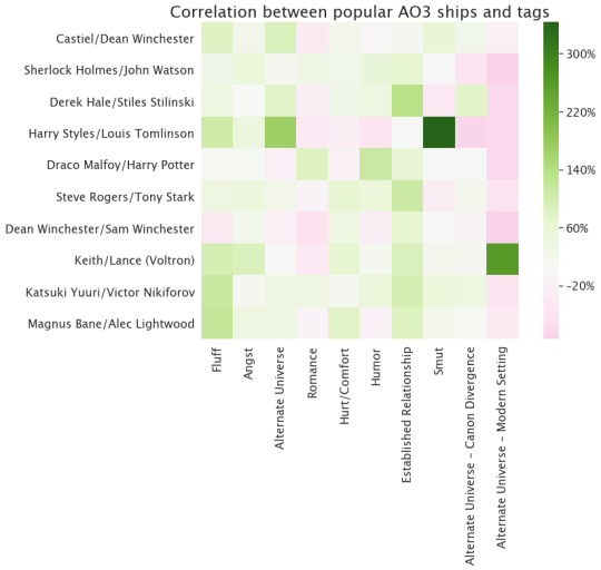
Okay, that’s...less interesting than I was expecting. Lots of Harry/Louis smut, lots of Keith/Lance modern AUs. The most likely established relationship is Derek/Stiles. Magnus/Alex and Yuuri/Victor are the fluffiest. Not much romance, except for Draco/Harry, and that pairing also has an unusual amount of humor.

What about character tags?

Hmm. Looks like there are a lot of teen-rated Marvel works, and Supernatural leans towards the higher ratings (which we already knew).

This basically just repeats stuff we already noticed in the relationships plot, I think. One thing I didn’t notice up there is that John and Sherlock are not that likely to be tagged in Established Relationship works, which is kind of interesting as they’re long-term partners (not necessarily romantic partners) in most versions of the canon.

How about characters and pairing type...are there characters that appear more often in one kind of pairing than you'd expect based on randomness? (Note that all these characters appear most in M/M stories, because those are by far the most common--this is just asking a relative question about how much they appear in other kinds of stories.)

Mostly not super interesting, I have to say. Steve, Tony, Natasha, and Harry Potter are all more likely than usual to appear in poly relationships or in F/M stories, apparently, and Stiles and Castiel are less likely than usual to appear in gen works.

Finally, a really fun thing (that I have to link to an external site to do, because tumblr doesn’t like javascript in posts). Instead of just looking at the top 10 tags, here are the top 100 tags portrayed as dots, arranged in a connected graph: the dots represent tags (with the popularity of the tag represented by its size), and they’re connected by lines whose thickness indicates how often the two things appear together, relative to chance. You can also use this kind of setup to work out sets of interconnected tags that are more closely tied to each other than to the other tags. I colored those sets with different colors, so you can identify them. Hovering your mouse pointer over a dot should tell you which tag it is.

Here are the blocks of tags that the algorithm found:

Alternate Universe, Alternate Universe - College/University, Alternate Universe - High School, Alternate Universe - Human, Alternate Universe - Modern Setting, Alternate Universe - Soulmates, Christmas, Crack, Cute, Domestic Fluff, Fluff, Fluff And Humor, Humor, Light Angst, One Shot, Romance, Tooth-Rotting Fluff

Angst, Blood, Canon-Typical Violence, Canonical Character Death, Character Death, Dark, Death, Depression, Emotional Hurt/Comfort, Grief/Mourning, Hurt/Comfort, I'm Sorry, Magic, Minor Character Death, Nightmares, Post-Traumatic Stress Disorder - PTSD, Sad, Self-Harm, Suicidal Thoughts, Torture, Violence

Action/Adventure, Alternate Universe - Canon Divergence, Canon Compliant, Character Study, Crossover, Drabble, Drama, Family, Friendship, Future Fic, Post-Canon, Pre-Slash, Spoilers

Alcohol, Alpha/Beta/Omega Dynamics, Established Relationship, Explicit Language, Explicit Sexual Content, First Time, Fluff And Smut, Jealousy, Kissing, Mpreg, Polyamory, Sex, Sexual Content, Slash, Smut

Anal Fingering, Anal Sex, Bdsm, Blow Jobs, Bondage, Dirty Talk, Dom/Sub, Dubious Consent, Hand Jobs, Masturbation, Oral Sex, Plot What Plot/Porn Without Plot, Rimming, Rough Sex, Spanking

Angst With A Happy Ending, Developing Relationship, Eventual Smut, Falling In Love, First Kiss, Fluff And Angst, Friends To Lovers, Friendship/Love, Happy Ending, Implied Sexual Content, Love, Love Confessions, Mutual Pining, Other Additional Tags To Be Added, Pining, Slow Build, Slow Burn, Swearing, Unrequited Love

I love this! To me, those sets look like: fluffy plot-based tags, violence and disturbing content tags, more action-oriented plot-based tags, less explicit vanilla-ish erotica tags, more explicit or kinky erotica tags, and romance. That’s so cool. (Not everything makes sense--why is Drabble where it is?--but still, cool.)

Or in other words: some numerical routines correctly identified the porn. :)

Up next: what gets kudos?

#fan stats #ao3 #fanstats

32 notes · View notes

purnimacbse-blog · 6 years ago

Text

NCERT Solutions for Class 12 Maths Chapter 3 Matrices

NCERT Solutions for class 12 Maths Chapter 3 – Matrices, provides solutions for all the questions enlisted under the chapter (All Exercises and Miscellaneous Exercise solutions). Class 12 maths NCERT Solutions are solved by maths experts using step by step approach under the guidelines of NCERT to assists students in their examination. This topic is extremely important for both CBSE board exam and for competitive exams. Students can practice these questions and improve their skills. Download free NCERT Solutions pdf now and excel your knowledge.

In Class 12 Maths Chapter 3, students will deal with matrices and their types, properties, order of a matrix , operations on matrices (addition, multiplication), transpose of matrix, symmetric and skew-symmetric matrices, elementary operation (transformation) of a matrix, invertible matrices and inverse of a matrix by elementary operations. Students can practice problems on these topics and get ready for the exam.

NCERT Solutions For Class 12 Maths Chapter 3 Exercises:

Get detailed solution for all the questions listed under below exercises:

Exercise 3.1 Solutions : 10 Questions (7 Short Answers, 3 MCQ)

Exercise 3.2 Solutions : 22 Questions(14 Long, 6 Short, 2 MCQ)

Exercise 3.3 Solutions : 12 Questions (10 Short Answers, 2 MCQ)

Exercise 3.4 Solutions : 18 Questions (4 Long, 13 Short, 1 MCQ)

Miscellaneous Exercise Solutions: 15 Questions (7 Long, 5 Short, 3 MCQ)

#NCERT Solutions for Class 12 Maths Chapter 3

6 notes · View notes

dream2503 · 2 years ago

Text

class Matrix():

def matrix():

print("""All functions-

- Matrix.addition(m1, m2)

- Matrix.identity(m)

- Matrix.input()

- Matrix.isSkewSymmetric(m)

- Matrix.isSymmetric(m)

- Matrix.multiplication(m1, m2)

- Matrix.null(m, n)

- Matrix.order(m)

- Matrix.print(m)

- Matrix.scalarMultiplication(n, m)

- Matrix.subtraction(m1, m2)

- Matrix.transpose(m)""")

def addition(m1, m2):

"""Add two matrix and returns the resultant matrix"""

"""REQUIRES - Matrix.null, Matrix.order"""

if type(m1)==list and type(m2)==list:

order1=Matrix.order(m1)

order2=Matrix.order(m2)

if order1==order2:

L=Matrix.null(order1[0], order1[1])

for i in range(order1[0]):

for j in range(order2[1]):

L[i][j]+=m1[i][j]+m2[i][j]

else:

return 'Invalid order for addition'

else:

return 'Invalid matrix'

return L

def identity(m, n=1):

"""Creates a identity matrix of 1 (default) for given order"""

"""REQUIRES - Matrix.null"""

if type(m)==int:

L=Matrix.null(m)

for i in range(m):

for j in range(m):

if i==j:

L[i][j]=n

else:

return 'Invalid input'

return L

def input(m, n=None):

"""Creates a matrix of given order and returns the matrix """

if type(m)==int:

if n==None:

n=m

elif type(n)!=int:

return 'Invalid order'

L=[]

�� for i in range(m):

row=eval(input(f'Enter {i+1}th row ([x, y, z]): '))

if len(row)==n:

L.append(row)

else:

return 'Invalid matrix elements'

else:

return 'Invalid order input'

return L

def isSkewSymmetric(m):

"""Checks if the given matrix is skew symmetric and returns a boolean value"""

"""REQUIRES - Matrix.scalarMultiplication, Matrix.transpose"""

if type(m)==list and type(m[0])==list and len(m)==len(m[0]):

if m==Matrix.scalarMultiplication(-1, Matrix.transpose(m)):

return True

else:

return False

else:

return 'invalid square matrix'

def isSymmetric(m):

"""Checks if the given matrix is symmetric and returns a boolean value"""

"""REQUIRES - Matrix.transpose"""

if type(m)==list and type(m[0])==list and len(m)==len(m[0]):

if m==Matrix.transpose(m):

return True

else:

return False

else:

return 'Invalid square matrix'

def multiplication(m1, m2):

"""Multiplies two matrix and returns the resultant matrix"""

"""REQUIRES - Matrix.null, Matrix.order"""

if type(m1)==list and type(m2)==list:

order1=Matrix.order(m1)

order2=Matrix.order(m2)

if order1[1]==order2[0]:

L=Matrix.null(order1[0], order2[1])

for k in range(order1[0]):

for i in range(order2[1]):

for j in range(order1[0]):

L[k][i]+=m1[k][j]*m2[j][i]

else:

return 'Invalid matrix order to multiply'

else:

return 'Invalid matrix'

return L

def null(m, n=None):

"""Creates a null matrix for given order and returns the matrix"""

if type(m)==int:

if n==None:

n=m

elif type(n)!=int:

return 'Invalid order'

L=[]

for i in range(m):

L.append([])

for j in range(n):

L[i].append(0)

else:

return 'Invalid input'

return L

def order(m):

"""Returns the order of the given matrix"""

if type(m)==list and type(m[0])==list:

return [len(m), len(m[0])]

else:

return 'Invalid matrix'

def print(m):

"""Prints the given matrix"""

if type(m)==list and type(m[0])==list:

for i in range(len(m)):

print(m[i])

def scalarMultiplication(n, m):

"""Multiplies a matrix with a scalar value and returns the resultant matrix"""

"""REQUIRES - Matrix.null, Matrix.order"""

if type(n) in (int, float) and type(m)==list:

order=Matrix.order(m)

L=Matrix.null(order[0], order[1])

for i in range(order[0]):

for j in range(order[1]):

L[i][j]+=n*m[i][j]

else:

return 'Invalid matrix or scalar value'

return L

def subtraction(m1, m2):

"""Subtract two matrix and returns the resultant matrix"""

"""REQUIRES - Matrix.null, Matrix.order"""

if type(m1)==list and type(m2)==list:

order1=Matrix.order(m1)

order2=Matrix.order(m2)

if order1==order2:

L=Matrix.null(order1[0], order1[1])

for i in range(order1[0]):

for j in range(order2[1]):

L[i][j]+=m1[i][j]-m2[i][j]

else:

return 'Invalid order for substraction'

else:

return 'Invalid matrix'

return L

def transpose(m):

"""Returns the transpose of the given matrix"""

"""REQUIRES - Matrix.null, Matrix.order"""

if type(m)==list and type(m[0])==list and len(m)==len(m[0]):

order=Matrix.order(m)

order=order[0]

L=Matrix.null(order)

for i in range(order):

for j in range(order):

L[j][i]=m[i][j]

else:

return 'invalid square matrix'

return L

1 note · View note

pius2017 · 4 years ago

Text

A square matrix is called skew-symmetric if AT = -A. (a) (4 points) Explain why the main diagonal of a skew-symmetric matrix consists entirely of zeros

A square matrix is called skew-symmetric if AT = -A. (a) (4 points) Explain why the main diagonal of a skew-symmetric matrix consists entirely of zeros. (b) (2 points) Provide examples of a 2 x 2 skew-symmetric matrix and a 3 x 3 skew-symmetric matrix. (6 points) Prove that if A and B are both n x n skew-symmetric matrices and c is a nonzero scalar, then A + B and cA are both skew-symmetric as…

View On WordPress

0 notes

sautya · 4 years ago

Text

Finite Element Analysis - MCQ

Finite Element Analysis – MCQ

Finite Element Analysis – MCQ 1. Stiffness matrix is a a) Symmetric matrix.b) Skew symmetric matrix.c) Adjoining matrix.d) Augmented matrix. View Answer a) Symmetric matrix. Stiffness matrix is a symmetric matrix. 2. The local x-axis of a member is always parallel to the ____ of the member. a) Longitudinal axis.b) Vertical axis.c) Transverse axis.d) Horizontal axis. View Answer a)…

View On WordPress

0 notes

reeiiedu · 5 years ago

Text

Determinants

Determinant

Every square matrix A is associated with a number, called its determinant and it is denoted by det (A) or |A| .

Only square matrices have determinants. The matrices which are not square do not have determinants

(i) First Order Determinant

If A = [a], then det (A) = |A| = a

(ii) Second Order Determinant

|A| = a11a22 – a21a12

(iii) Third Order Determinant

Evaluation of Determinant of Square Matrix of Order 3 by Sarrus Rule

then determinant can be formed by enlarging the matrix by adjoining the first two columns on the right and draw lines as show below parallel and perpendicular to the diagonal.

The value of the determinant, thus will be the sum of the product of element. in line parallel to the diagonal minus the sum of the product of elements in line perpendicular to the line segment. Thus,

Δ = a11a22a33 + a12a23a31 + a13a21a32 – a13a22a31 – a11a23a32 – a12a21a33.

Note This method doesn’t work for determinants of order greater than 3.

Properties of Determinants

(i) The value of the determinant remains unchanged, if rows are changed into columns and columns are changed into rows e.g.,

|A’| = |A|

(ii) If A = [aij]n x n , n > 1 and B be the matrix obtained from A by interchanging two of its rows or columns, then

det (B) = – det (A)

(iii) If two rows (or columns) of a square matrix A are proportional, then |A| = O.

(iv) |B| = k |A| ,where B is the matrix obtained from A, by multiplying one row (or column) of A by k.

(v) |kA| = kn|A|, where A is a matrix of order n x n.

(vi) If each element of a row (or column) of a determinant is the sum of two or more terms, then the determinant can be expressed as the sum of two or more determinants, e.g.,

(vii) If the same multiple of the elements of any row (or column) of a determinant are added to the corresponding elements of any other row (or column), then the value of the new determinant remains unchanged, e.g.,

(viii) If each element of a row (or column) of a determinant is zero, then its value is zero.

(ix) If any two rows (columns) of a determinant are identical, then its value is zero.

(x) If each element of row (column) of a determinant is expressed as a sum of two or more terms, then the determinant can be expressed as the sum of two or more determinants.

Important Results on Determinants

(i) |AB| = |A||B| , where A and B are square matrices of the same order.

(ii) |An| = |A|n

(iii) If A, B and C are square matrices of the same order such that ith column (or row) of A is the sum of i th columns (or rows) of B and C and all other columns (or rows) of A, Band C are identical, then |A| =|B| + |C|

(iv) |In| = 1,where In is identity matrix of order n

(v) |On| = 0, where On is a zero matrix of order n

(vi) If Δ(x) be a 3rd order determinant having polynomials as its elements.

(a) If Δ(a) has 2 rows (or columns) proportional, then (x – a) is a factor of Δ(x).

(b) If Δ(a) has 3 rows (or columns) proportional, then (x – a)2 is a factor of Δ(x). ,

(vii) A square matrix A is non-singular, if |A| ≠ 0 and singular, if |A| =0.

(viii) Determinant of a skew-symmetric matrix of odd order is zero and of even order is a non-zero perfect square.

(ix) In general, |B + C| ≠ |B| + |C|

(x) Determinant of a diagonal matrix = Product of its diagonal elements

(xi) Determinant of a triangular matrix = Product of its diagonal elements

(xii) A square matrix of order n, is non-singular, if its rank r = n i.e., if |A| ≠ 0, then rank (A) = n

(xiv) If A is a non-singular matrix, then |A-1| = 1 / |A| = |A|-1

(xv) Determinant of a orthogonal matrix = 1 or – 1.

(xvi) Determinant of a hermitian matrix is purely real .

(xvii) If A and B are non-zero matrices and AB = 0, then it implies |A| = 0 and |B| = 0.

Minors and Cofactors

then the minor Mij of the element aij is the determinant obtained by deleting the i row and jth column.

The cofactor of the element aij is Cij = (- 1)i + j Mij

Adjoint of a Matrix – Adjoint of a matrix is the transpose of the matrix of cofactors of the give matrix, i.e.,

Properties of Minors and Cofactors

(i) The sum of the products of elements of .any row (or column) of a determinant with the cofactors of the corresponding elements of any other row (or column) is zero, i.e., if

then a11C31 + a12C32 + a13C33 = 0 ans so on.

(ii) The sum of the product of elements of any row (or column) of a determinant with the cofactors of the corresponding elements of the same row (or column) is Δ

Differentiation of Determinant

Integration of Determinant

If the elements of more than one column or rows are functions of x, then the integration can be done only after evaluation/expansion of the determinant.

Solution of Linear equations by Determinant/Cramer’s Rule

Case 1. The solution of the system of simultaneous linear equations

a1x + b1y = C1 …(i)

a2x + b2y = C2 …(ii)

is given by x = D1 / D, Y = D2 / D

(i) If D ≠ 0, then the given system of equations is consistent and has a unique solution given by x = D1 / D, y = D2 / D

(ii) If D = 0 and Dl = D2 = 0, then the system is consistent and has infinitely many solutions.

(iii) If D = 0 and one of Dl and D2 is non-zero, then the system is inconsistent.

Case II. Let the system of equations be

a1x + b1y + C1z = d1

a2x + b2y + C2z = d2

a3x + b3y + C3z = d3

Then, the solution of the system of equation is

x = D1 / D, Y = D2 / D, Z = D3 / D, it is called Cramer’s rule.

(i) If D ≠ 0, then the system of equations is consistent with unique solution.

(ii) If D = 0 and atleast one of the determinant D1, D2, D3 is non-zero, then the given system is inconsistent, i.e., having no solution.

(iii) If D = 0 and D1 = D2 = D3 = 0, then the system is consistent, with infinitely many solutions.

(iv) If D ≠ 0 and D1 = D2 = D3 = 0, then system has only trivial solution, (x = y = z = 0).

Cayley-Hamilton Theorem

Every matrix satisfies its characteristic equation, i.e., if A be a square matrix, then |A – xl| = 0 is the characteristics equation of A. The values of x are called eigenvalues of A.

i.e., if x3 – 4x2 – 5x – 7 = 0 is characteristic equation for A, then

A3 – 4A2 + 5A – 7I = 0

Properties of Characteristic Equation

(i) The sum of the eigenvalues of A is equal to its trace.

(ii) The product of the eigenvalues of A is equal to its determinant.

(iii) The eigenvalues of an orthogonal matrix are of unit modulus.

(iv) The feigen values of a unitary matrix are of unit modulus.

(v) A and A’ have same eigenvalues.

(vi) The eigenvalues of a skew-hermitian matrix are either purely imaginary or zero.

(vii) If x is an eigenvalue of A, then x is the eigenvalue of A* .

(viii) The eigenvalues of a triangular matrix are its diagonal elements.

(ix) If x is the eigenvalue of A and |A| ≠ 0, then (1 / x) is the eigenvalue of A-1.

(x) If x is the eigenvalue of A and |A| ≠ 0, then |A| / x is the eigenvalue of adj (A).

(xi) If x1, x2,x3, … ,xn are eigenvalues of A, then the eigenvalues of A2 are x22, x22,…, xn2.

Cyclic Determinants

Applications of Determinant in Geometry

Let three points in a plane be A(x1, y1), B(x2, y2) and C(x3, y3), then

= 1 / 2 [x1 (y2 – y3) + x2 (y3 – y1) + x3 (y1 – y2)]

Maximum and Minimum Value of Determinants

where ais ∈ [α1, α2,…, αn]

Then, |A|max when diagonal elements are

{ min (α1, α2,…, αn)}

and non-diagonal elements are

{ max (α1, α2,…, αn)}

Also, |A|min = – |A|max

0 notes

craigbrownphd-blog-blog · 5 years ago

Text

If you did not already know

Scaled Cayley Orthogonal Recurrent Neural Network (scoRNN) Recurrent Neural Networks (RNNs) are designed to handle sequential data but suffer from vanishing or exploding gradients. Recent work on Unitary Recurrent Neural Networks (uRNNs) have been used to address this issue and in some cases, exceed the capabilities of Long Short-Term Memory networks (LSTMs). We propose a simpler and novel update scheme to maintain orthogonal recurrent weight matrices without using complex valued matrices. This is done by parametrizing with a skew-symmetric matrix using the Cayley transform. Such a parametrization is unable to represent matrices with negative one eigenvalues, but this limitation is overcome by scaling the recurrent weight matrix by a diagonal matrix consisting of ones and negative ones. The proposed training scheme involves a straightforward gradient calculation and update step. In several experiments, the proposed scaled Cayley orthogonal recurrent neural network (scoRNN) achieves superior results with fewer trainable parameters than other unitary RNNs. … gcForest In this paper, we propose gcForest, a decision tree ensemble approach with performance highly competitive to deep neural networks. In contrast to deep neural networks which require great effort in hyper-parameter tuning, gcForest is much easier to train. Actually, even when gcForest is applied to different data from different domains, excellent performance can be achieved by almost same settings of hyper-parameters. The training process of gcForest is efficient and scalable. In our experiments its training time running on a PC is comparable to that of deep neural networks running with GPU facilities, and the efficiency advantage may be more apparent because gcForest is naturally apt to parallel implementation. Furthermore, in contrast to deep neural networks which require large-scale training data, gcForest can work well even when there are only small-scale training data. Moreover, as a tree-based approach, gcForest should be easier for theoretical analysis than deep neural networks. … JMP SAS created JMP in 1989 to empower scientists and engineers to explore data visually. Since then, JMP has grown from a single product into a family of statistical discovery tools, each one tailored to meet specific needs. All of our software is visual, interactive, comprehensive and extensible. … PArameterized Clipping acTivation (PACT) Deep learning algorithms achieve high classification accuracy at the expense of significant computation cost. To address this cost, a number of quantization schemes have been proposed – but most of these techniques focused on quantizing weights, which are relatively smaller in size compared to activations. This paper proposes a novel quantization scheme for activations during training – that enables neural networks to work well with ultra low precision weights and activations without any significant accuracy degradation. This technique, PArameterized Clipping acTivation (PACT), uses an activation clipping parameter $\alpha$ that is optimized during training to find the right quantization scale. PACT allows quantizing activations to arbitrary bit precisions, while achieving much better accuracy relative to published state-of-the-art quantization schemes. We show, for the first time, that both weights and activations can be quantized to 4-bits of precision while still achieving accuracy comparable to full precision networks across a range of popular models and datasets. We also show that exploiting these reduced-precision computational units in hardware can enable a super-linear improvement in inferencing performance due to a significant reduction in the area of accelerator compute engines coupled with the ability to retain the quantized model and activation data in on-chip memories. … https://bit.ly/31uiYor

0 notes

mamtajuyal1986 · 6 years ago

Text

IIT JAM 2020 Mathematical Statistics (MS) Syllabus | IIT JAM 2020 Mathematical Statistics (MS) Exam Pattern

IIT JAM 2020 Mathematical Statistics (MS) Syllabus | IIT JAM 2020 Mathematical Statistics (MS) Exam Pattern Mathematical Statistics (MS): The syllabus is a very important aspect while preparing for the examination. Therefore it is advised to all the appearing candidates that they should go through the Mathematical Statistics (MS) syllabus properly before preparing for the examination. The Mathematical Statistics (MS) test paper comprises of Mathematics (40% weightage) and Statistics (60%weightage). MATHEMATICS Sequences and Series: Convergence of sequences of real numbers, Comparison, root and ratio tests for convergence of series of real numbers. Differential Calculus: Limits, continuity and differentiability of functions of one and two variables. Rolle's theorem, mean value theorems, Taylor's theorem, indeterminate forms, maxima and minima of functions of one and two variables. Integral Calculus: Fundamental theorems of integral calculus. Double and triple integrals, applications of definite integrals, arc lengths, areas and volumes. Matrices: Rank, inverse of a matrix. Systems of linear equations. Linear transformations, eigenvalues and eigenvectors. Cayley-Hamilton theorem, symmetric, skew-symmetric and orthogonal matrices. STATISTICS Probability: Axiomatic definition of probability and properties, conditional probability, multiplication rule. Theorem of total probability. Bayes' theorem and independence of events. Random Variables: Probability mass function, probability density function and cumulative distribution functions, distribution of a function of a random variable. Mathematical expectation, moments and moment generating function. Chebyshev's inequality. Standard Distributions: Binomial, negative binomial, geometric, Poisson, hypergeometric, uniform, exponential, gamma, beta and normal distributions. Poisson and normal approximations of a binomial distribution. Joint Distributions: Joint, marginal and conditional distributions. Distribution of functions of random variables. Joint moment generating function. Product moments, correlation, simple linear regression. Independence of random variables. Sampling Distributions: Chi-square, t and F distributions, and their properties. Limit Theorems: Weak law of large numbers. Central limit theorem (i.i.d.with finite variance case only). Estimation: Unbiasedness, consistency and efficiency of estimators, method of moments and method of maximum likelihood. Sufficiency, factorization theorem. Completeness, Rao-Blackwell and Lehmann-Scheffe theorems, uniformly minimum variance unbiased estimators. Rao-Cramer inequality. Confidence intervals for the parameters of univariate normal, two independent normal, and one parameter exponential distributions. Testing of Hypotheses: Basic concepts, applications of Neyman-Pearson Lemma for testing simple and composite hypotheses. Likelihood ratio tests for parameters of univariate normal distribution. Related Articles: IIT JAM 2020 Syllabus Biotechnology (BT) Syllabus Biological Sciences (BL) Syllabus Chemistry (CY) Syllabus Geology (GG) Syllabus Mathematics (MA) Syllabus Mathematical Statistics (MS) Syllabus Physics (PH) Syllabus Read the full article

#IITJAM2020 #IITJAM2020MSSyllabus #IITJAM2020Syllabus

0 notes

twocubes · 6 years ago

Text

Aha!

I have managed to prove the conservation of angular momentum for n-dimensional rigid body mechanics.

Though, as expected, the angular momentum is now an arbitrary skew-symmetric matrix, which ultimately translates to free rotation doing that thing I talked about forever ago, where your rigid object is freely spinning along floor(n/2) mutually orthogonal planes of rotation at unrelated speeds...

Now I have to figure out... n-dimensional torque, I guess? Derivative of a matrix, right, it’s gotta be, so... another antisymmetric matrix. But... then if you poke the body, how does it spin?

...

Hm. I think I see it, but I have to think.

Tomorrow tho it’s bedtimes now...

I wonder how precession works in 4/5d Newtonian mechanics...

35 notes · View notes

pius2017 · 4 years ago

Text

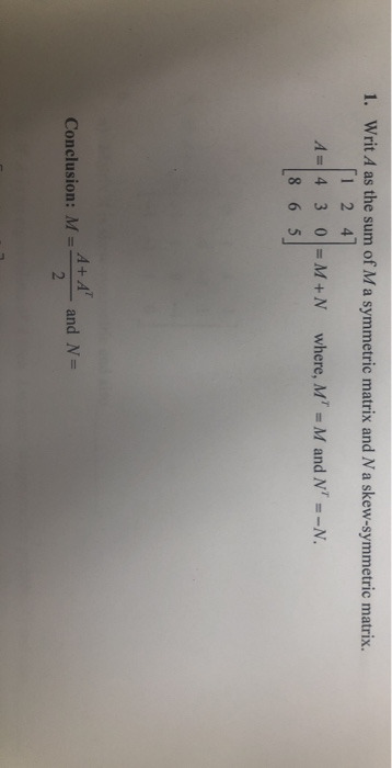
Write A as the sum of Ma symmetric matrix and Na skew-symmetric matrix

1. Write A as the sum of Ma symmetric matrix and Na skew-symmetric matrix. 1 24 A=430= M+N 865 where, MT M and N-N. A+A Conclusion: M = and N= 2

View On WordPress

0 notes

craigbrownphd · 5 years ago

Text

If you did not already know

0 notes

eigenx-blog · 5 years ago

Text