#subtraction of matrices

[pandoramsbox]

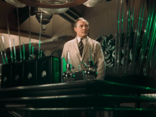
Sci-Fi Saturday: Doctor X

Week 8:

Film(s): Doctor X (Dir. Michael Curtiz, 1932)

Viewing Format: DVD

Date Watched: July 2, 2021

Rationale for Inclusion:

As mentioned last week, the critical and box office success of Frankenstein (Dir. James Whale, 1931, USA) resulted in a rush to make additional horror and/or mad scientist films. This trend would slow after 1934, in part because the beginning of enforcement of the Motion Picture Production Code sought to limit gruesome and violent content in American movies. The following weeks will include a handful of noteworthy examples of Pre-Code horror sci-fi. The first is Doctor X (Dir. Michael Curtiz, 1932, USA).

The main reason I included Doctor X in this survey, other than being a fan of the film, is that it was shot in two-color Technicolor. The color system, often incorrectly called "two-strip Technicolor", was the third iteration of the Technicolor motion picture color process. The color images produced originated on black and white film where each frame was captured first through a red filter, then a green one. Separate red and green color matrices would be created, dyed cyan-green and orange-red respectively, and in combination during the dye imbibition printing process created semi-realistic color images. 

It's only "semi-realistic" because blues and purples are not reproduced, thus not replicating all colors perceivable to the human eye. This lack would soon be corrected by adding a third color matrix in the fourth iteration of the process: three-strip Technicolor, the famous "glorious Technicolor" of mid-century Hollywood and British cinema.

Part of the joy of going through science fiction cinema chronologically is watching technology advance over time. So far we've gone from silent to sound, and with Doctor X we introduce the first film of the survey shot with a subtractive color process.

Reactions:

Despite the overly elaborate lie-detector and laboratory set pieces in play, Doctor X is more of a horror film than a science fiction one. The main group of characters is a group of scientists and their leader Doctor Xavier (Lionel Atwill) uses a scientific contraption to suss out which of his colleagues is the allegedly cannibalistic serial killer on the loose, but the plot is more concerned with the crimes of the allegedly cannibalistic serial killer on the loose. The film also includes a beautiful woman being menaced by the reporter investigating Doctor Xavier's connection to the crimes, Lee Taylor (Lee Tracy), and the actual killer, in the form of a dark haired Fay Wray, as Doctor Xavier's daughter Joanne. Even before her legacy defining performance in King Kong (Dir. Merian C. Cooper and Ernest B. Schoedsack, 1933, USA), Wray was an established scream queen.

As the film goes on it is revealed that the serial killer was not taking away parts of his victims to eat, as originally thought, but as research samples for creating synthetic flesh. This synthetic flesh can also apparently create muscles, tendons, bones, capillaries and all the other complex structures of the human body because, in addition to using his invention to disguise his face, the killer fashions a fully functional synthetic arm from the magical puddy. It's a shame that this technology is limited to a plot point instead of a core part of the narrative because it is conceptually fascinating. I suppose that's what Clayface plotlines in Batman media are for though.

Interestingly from a production and trivia standpoint is the fact that the horror effects make-up for the synthetic flesh was created by Max Factor. The company was known for its innovations in cosmetics with the specific demands of cinematic production in mind, but its focus was on creating beauty, not monsters. Granted, even Universal Studios' maestro of monsters Jack Pierce had a workload of applying mostly conventional beauty make-up. Specialists in special effects make-up, like Rick Baker, would not exist until after the disillusionment of the studio system.

The Technicolor shows off its ability to display color, but does not descend into what I call "Technicolor abuse," which I define as the use of color for spectacle more than contributing to the overall diegesis of the film. (For examples of Technicolor Abuse see The Adventures of Robin Hood (Dir. Michael Curtiz, 1938, USA) and Babes in Toyland (Dir. Jack Donohue, 1961, USA)) Given the overall emphasis on green in the film's color palette, the red heart beating in the jar in Dr. Wells' (Preston Foster) lab adds to the intended shock value of the moment. Cinematographer Ray Rennahan makes the most of two-color Technicolor's limited range to create beautifully composed, vivid scenes.Doctor X may be more horror than sci-fi, but it's still an entertaining genre flick. It was successful enough at the box office to result in Warner Brothers Studios making a follow up film again starring Atwill and Wray, with direction by Curtiz and Technicolor cinematography by Rennahan, The Mystery of the Wax Museum (1933). Like Doctor X it shows off two-color Technicolor at its best, but unlike its predecessor it's pure horror.

[algebra-as-praxis]

First post!! I wanted to show you how deep a rabbit hole you can dig with a very simple concept like, "What does 'four' mean?"

I have a number line.

So, I'd like you to imagine that you've sat down across from me on your first day in class, and I put some kind of math worksheet with this number line on it that gives you a very simple-sounding task: "Circle four."

If you are like nearly every one of the older students I've had, you'll circle the number 4 on the line. And I'd say something like, "That is a perfectly reasonable response to this request. There is nothing wrong with what you've done. But aren't you suspicious about how simple this question sounds? Did you see that there was a twist coming?"

On a number line, the place where we've written 4 is not actually the value 4. It is more like the position 4; we would call this the ordinal number (a number used to track the positional order of things; another example of an ordinal number is the word "fourth," which tells you that there are three other things before that one).

So, if you just circled the number 4, you definitely circled the position, but the thing you circled isn't worth 4. If you were going to circle the thing that has the value (or cardinality, since we're counting individual objects) of 4, it would look something more like this:

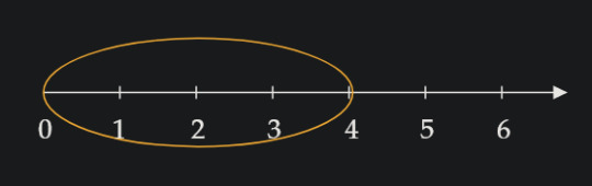
This is because in order to have the value of 4, you need everything that came before it! Imagine counting out candy while your kid sister steals and eats the candies you counted already. When you get to your final number, that number is not how many candies you have, but rather how many you counted cuz your sister's got 'em all! For the value of your candies to stay the same, you need all of them to be there!

"Four" could also look, less straightforwardly, like this:

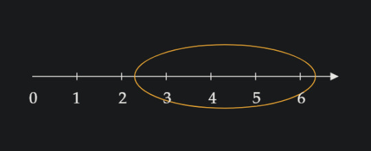
The distance from the start of the circle to the end is four; and since we're circling the line, the length of the line that is circled is four. If we imagine the circle starts (from the left) at the position of 2.3, it would have to end at the position (from the right) 6.3. If we find the difference of the numbers at these positions, we would be doing the equation 6.3 - 2.3 = 4.

A quick summary:

The position of a number is shown with an ordinal number.

The actual physical quantity of the individual items is shown with a cardinal number, which we more typically call the value.

We can find a value inside the ordinals by finding the distance between any two ordinals, via subtraction.

Okay... But notice we've used two words here that seem to imply the same thing: difference and distance. Let's clear this up real quick:

Difference is the result of subtraction. Generally, if we want to find the difference between two things, we subtract the first thing from the second thing:

second - first = difference

But that's not a rule, so much as a norm. In reality, if you wanted to find the difference of two numbers, the person asking had best be very clear which way they want you to do it, because if you reverse this you will get the negative of the result above!

For example, if you were asked to find the difference between 6 and 15, you would do 15 - 6 = 9. But if it's not clear and you instead did 6 - 15, you get -9.

If, however, someone wanted to know how far apart these two numbers are, they would not be asking the difference but rather the distance between these numbers. The result would therefore be the absolute value of either one of these subtractions:

|15 - 6| = |9| = 9, |6 - 15| = |-9| = 9 Same result!

This is in actuality the real use of absolute values. Absolute value is typically shown as "the distance from zero," which is kind of true? But it's really for finding distances of any kind -- in fact, it's later used to mean exactly that when you get into complex algebra (that is, algebra with imaginary numbers) and linear algebra (matrices and vectors).

But that's for later.

[itpointonline]

Step-by-Step Python NumPy Tutorial with Real-Life Examples

If you are starting with Python and want to explore data science or numerical computing, then this Python NumPy Tutorial is perfect for you. NumPy stands for “Numerical Python” and is one of the most important libraries used in data analysis, scientific computing, and machine learning.

NumPy makes it easy to work with large sets of numbers. It provides a special data structure called an “array” that is faster and more efficient than regular Python lists. With NumPy arrays, you can perform many mathematical operations like addition, subtraction, multiplication, and more in just a few steps.

This Python NumPy Tutorial helps you understand the basics of arrays, data types, and array operations. It also introduces important features like indexing, slicing, and reshaping arrays. These features allow you to manage and process data in a smart and simple way.

NumPy also supports working with multi-dimensional data. This means you can handle tables, matrices, and higher-dimensional data easily. Whether you’re working with simple numbers or complex datasets, NumPy gives you the tools to analyze and manipulate them effectively.

In short, this tutorial is a great starting point for beginners. It breaks down complex concepts into easy steps, making it simple to understand and follow. If you're planning to learn data science or work with big data in Python, learning NumPy is a must.

To read the full tutorial, visit Python NumPy Tutorial.

[codingprolab]

Math 551 Lab 1

Goals: To learn and practice different forms of matrix input and basic operations with matrices in Matlab. The matrix operations to be studied include matrix addition and subtraction, scalar product, matrix product and elementwise matrix product in Matlab, matrix concatenation, and selecting submatrices. To get started: Create a new Matlab script file and save it as “lab01.m”. Matlab commands to…

[ankitcodinghub]

MATH208 - Programming Assignment IV Sparse Matrix Solved

1 Description of the Assignment Implement appropriate data structures to support efficient operations on sparse matrices. The operations should at least include addition (subtraction) and multiplication of matrices. 2 Input Provide at least the following method for input. 1. The dimensions of the matrix m × n. 2. List of the nonzero elements of each row. For example, let the matrix be The input…

[socialexpressions]

Data structures in R

R is a powerful language designed for statistical computing and data analysis, and one of its core strengths lies in its ability to handle complex data structures efficiently. Among these, vectors, matrices, and arrays are foundational. In this section, we’ll explore these data structures, understand how they are created, manipulated, and applied in various contexts.

Vectors in R

A vector is the simplest and most common data structure in R. It is a one-dimensional array that can hold numeric, character, or logical data types, but all elements in a vector must be of the same type.

Creating Vectors:

You can create a vector using the c() function, which combines values into a vector.# Numeric vector numeric_vector <- c(1, 2, 3, 4, 5) # Character vector character_vector <- c("apple", "banana", "cherry") # Logical vector logical_vector <- c(TRUE, FALSE, TRUE)

Accessing Elements:

You can access elements in a vector using square brackets [].# Access the first element numeric_vector[1] # Access multiple elements numeric_vector[c(1, 3, 5)]

Vectorized Operations:

One of the powerful features of vectors in R is vectorized operations. You can perform operations on entire vectors without needing explicit loops.# Adding 2 to each element numeric_vector + 2 # Element-wise multiplication of two vectors numeric_vector * c(2, 2, 2, 2, 2)

Matrices in R

A matrix is a two-dimensional array where elements are arranged in rows and columns. Like vectors, all elements in a matrix must be of the same type.

Creating Matrices:

You can create a matrix using the matrix() function by specifying the data, number of rows, and number of columns.# Creating a 2x3 matrix my_matrix <- matrix(1:6, nrow = 2, ncol = 3) # Display the matrix print(my_matrix)

This will produce:[,1] [,2] [,3] [1,] 1 3 5 [2,] 2 4 6

Accessing Elements:

You can access elements in a matrix using square brackets [] by specifying the row and column indices.# Access the element in the first row, second column my_matrix[1, 2] # Access the entire second row my_matrix[2, ]

Matrix Operations:

R supports a variety of matrix operations, such as addition, subtraction, multiplication, and more.# Matrix addition matrix1 <- matrix(1:4, nrow = 2) matrix2 <- matrix(5:8, nrow = 2) matrix_sum <- matrix1 + matrix2 # Matrix multiplication matrix_product <- matrix1 %*% matrix2

Arrays in R

An array in R is a multi-dimensional generalization of matrices. While matrices are restricted to two dimensions, arrays can have more than two dimensions.

Creating Arrays:

You can create an array using the array() function by specifying the data and the dimensions.# Creating a 3-dimensional array my_array <- array(1:12, dim = c(2, 3, 2)) # Display the array print(my_array)

This creates a 2x3x2 array. The first dimension has 2 rows, the second has 3 columns, and the third has 2 layers.

Accessing Elements:

Similar to matrices, you can access elements in an array using square brackets, but with additional indices for higher dimensions.# Access the element in the first row, second column of the first layer my_array[1, 2, 1] # Access all elements in the second layer my_array[ , , 2]

Practical Applications of Vectors, Matrices, and Arrays

These data structures are central to many data science and statistical tasks in R:

Vectors: Used for storing and manipulating sequences of data, such as time series or categorical variables.

Matrices: Commonly used in linear algebra, where you might perform matrix multiplication, inversion, or eigenvalue decomposition.

Arrays: Useful in more complex scenarios, such as handling 3D data in image processing or multi-dimensional statistical models.

Best Practices

Consistency in Data Types: Ensure that all elements within a vector, matrix, or array are of the same data type to avoid unexpected errors or results.

Vectorization: Whenever possible, leverage R's vectorized operations for better performance and cleaner code.

Dimensional Clarity: When working with matrices and arrays, clearly understand and manage the dimensions to ensure accurate data manipulation.

See the complete article at https://strategicleap.blogspot.com/

[lmerli2953]

Basics of R programming

Understanding the basics of R programming is crucial for anyone looking to leverage its capabilities for data analysis and statistical computing. In this chapter, we'll explore the fundamental elements of R, including its syntax, variables, data types, and operators. These are the building blocks of any R program and are essential for developing more complex scripts and functions.

R Syntax

R's syntax is designed to be straightforward and user-friendly, especially for those new to programming. It emphasizes readability and ease of use, which is why it's popular among statisticians and data scientists.

Comments: Comments are used to annotate code, making it easier to understand. In R, comments begin with a # symbol:# This is a comment in R

Statements and Expressions: R executes statements and expressions sequentially. Statements are typically written on separate lines, but multiple statements can be written on a single line using a semicolon (;):x <- 10 # Assigning a value to variable x y <- 5; z <- 15 # Multiple statements in one line

Printing Output: The print() function is commonly used to display the output of expressions or variables. Simply typing the variable name in the console will also display its value:print(x) # Displays the value of x x # Another way to display x

Variables in R

Variables are used to store data values in R. They are essential for performing operations, data manipulation, and storing results.

Creating Variables: Variables are created using the assignment operator <- or =. Variable names can contain letters, numbers, and underscores, but they must not start with a number:num <- 100 # Assigns the value 100 to the variable num message <- "Hello, R!" # Assigns a string to the variable message

Variable Naming Conventions: It’s good practice to use descriptive names for variables to make the code more readable:total_sales <- 500 customer_name <- "John Doe"

Accessing Variables: Once a variable is created, it can be used in expressions or printed to view its value:total_sales <- 1000 print(total_sales) # Outputs 1000

Data Types in R

R supports a variety of data types that are crucial for handling different kinds of data. The main data types in R include:

Numeric: Used for real numbers (e.g., 42, 3.14):num_value <- 42.5

Integer: Used for whole numbers. Integer values are explicitly declared with an L suffix:int_value <- 42L

Character: Used for text strings (e.g., "Hello, World!"):text_value <- "R programming"

Logical: Used for Boolean values (TRUE or FALSE):

is_active <- TRUE

Factors: Factors are used for categorical data and store both the values and their corresponding levels:status <- factor(c("Single", "Married", "Single"))

Vectors: Vectors are the most basic data structure in R, and they can hold elements of the same type:num_vector <- c(10, 20, 30, 40, 50)

Lists: Lists can contain elements of different types, including vectors, matrices, and even other lists:mixed_list <- list(num_value = 42, text_value = "R", is_active = TRUE)

Operators in R

Operators in R are used to perform operations on variables and data. They include arithmetic operators, relational operators, and logical operators.

Arithmetic Operators: These operators perform basic mathematical operations:

Addition: +

Subtraction: -

Multiplication: *

Division: /

Exponentiation: ^

Modulus: %% (remainder of division)

Example:a <- 10 b <- 3 sum <- a + b # 13 difference <- a - b # 7 product <- a * b # 30 quotient <- a / b # 3.3333 power <- a^b # 1000 remainder <- a %% b # 1

Relational Operators: These operators compare two values and return a logical value (TRUE or FALSE):

Equal to: ==

Not equal to: !=

Greater than: >

Less than: <

Greater than or equal to: >=

Less than or equal to: <=

Example:x <- 10 y <- 5 is_greater <- x > y # TRUE is_equal <- x == y # FALSE

Logical Operators: Logical operators are used to combine multiple conditions:

AND: &

OR: |

NOT: !

Example:a <- TRUE b <- FALSE both_true <- a & b # FALSE either_true <- a | b # TRUE not_a <- !a # FALSE

Working with Data Structures

Understanding R’s data structures is essential for manipulating and analyzing data effectively.

Vectors: As mentioned earlier, vectors are a fundamental data structure in R, and they are used to store sequences of data elements of the same type:numbers <- c(1, 2, 3, 4, 5)

Matrices: Matrices are two-dimensional arrays that store elements of the same type. You can create a matrix using the matrix() function:matrix_data <- matrix(1:9, nrow = 3, ncol = 3)

Data Frames: Data frames are used for storing tabular data, where each column can contain a different type of data. They are akin to tables in a database:df <- data.frame(Name = c("John", "Jane", "Doe"), Age = c(25, 30, 35))

Lists: Lists are versatile structures that can store different types of elements, including other lists:my_list <- list(name = "John", age = 30, scores = c(90, 85, 88))

Uncover more details at Strategic Leap

[careerguide1]

Key Linear Algebra Concepts Every Machine Learning Student in Pune Must Know

Linear algebra is a cornerstone for anyone studying machine learning, particularly for students enrolled in a machine learning course in Pune. It is a foundational subject that underpins many of the algorithms used in machine learning, making it essential for students to grasp its concepts. Whether you're pursuing a career in data science, artificial intelligence, or machine learning, a strong understanding of linear algebra will help you navigate complex models and improve your ability to work with data. Below, we’ll explore some key linear algebra concepts relevant to machine learning students in Pune.

1. Vectors and Vector Spaces

Vectors are one of the most fundamental concepts in linear algebra and are crucial in machine learning. A vector can be thought of as a list of numbers representing a point in space, such as a data point with several features. For example, if you're working on a dataset in your machine learning course in Pune, each row of the dataset can be considered a vector. Understanding vector operations like addition, scalar multiplication, and dot products is essential for tasks such as calculating distances between points and working with gradients in optimization problems.

In machine learning, vectors also represent weights in models like linear regression or neural networks. Mastering the concept of vectors and their operations will help you understand how machine learning algorithms function.

2. Matrices and Matrix Operations

In a machine learning course in Pune, students often deal with matrices, which are grids of numbers representing data or transformations. A matrix can be used to represent multiple vectors or a dataset. Matrix operations like addition, subtraction, and multiplication are vital for performing tasks such as transforming datasets, manipulating multi-dimensional data, and performing dimensionality reduction techniques like Principal Component Analysis (PCA).

Understanding how to work with matrices also helps in implementing algorithms like support vector machines (SVMs) and linear regression. For example, matrix multiplication can be used to calculate predictions in linear models more efficiently.

3. Eigenvalues and Eigenvectors

Eigenvalues and eigenvectors are fundamental in understanding many machine learning algorithms, particularly those involving dimensionality reduction. When working with large datasets in your machine learning course in Pune, one challenge is handling the high-dimensional feature space. Eigenvectors help to identify the principal directions in the data where the most variation occurs, allowing for dimensionality reduction.

Eigenvalues give a measure of the importance of each eigenvector in capturing the variance of the data. This concept is integral to algorithms like PCA, which reduce the number of features while retaining the most important information, making computations more efficient.

4. Singular Value Decomposition (SVD)

Singular Value Decomposition (SVD) is another powerful tool in linear algebra with applications in machine learning. It is used to decompose a matrix into three simpler matrices, allowing for easier calculations. SVD is often applied in recommendation systems, where the goal is to reduce large datasets (such as user-item matrices) into smaller, more manageable forms without losing too much information.

In a machine learning course in Pune, you’ll encounter SVD when working on advanced topics like collaborative filtering, which is used in recommendation engines. It is also employed in natural language processing tasks to reduce the dimensionality of word embeddings.

5. Linear Transformations

Linear transformations refer to functions that take vectors as inputs and return other vectors, typically by applying a matrix. This concept is crucial when dealing with data preprocessing steps like scaling, rotation, and translation. For example, in neural networks, transformations are performed on input data through layers of weights, which are matrices.

In the machine learning course in Pune, you will learn how to apply linear transformations to optimize model training and improve the performance of algorithms like logistic regression and deep learning models.

Conclusion

For students pursuing a machine learning training in Pune, a strong foundation in linear algebra is crucial for understanding the inner workings of machine learning algorithms. Concepts like vectors, matrices, eigenvalues, and SVD are not just theoretical but have practical applications in tasks ranging from data preprocessing to algorithm optimization. By mastering these concepts, you’ll be better equipped to work with the advanced techniques and tools required to succeed in machine learning.

[pandeypankaj]

What are the mathematical prerequisites for data science?

The key prerequisites for mathematics in Data Science would involve statistics and linear algebra.

Some of the important mathematical concepts one will encounter are as follows:

Statistics

 Probability Theory: Probability distributions should be known, particularly normal, binomial, and Poisson, with conditional probability and Bayes' theorem. These will come in handy while going through statistical models and machine learning algorithms.

Descriptive Statistics: Measures of central tendency, mean, median, and mode, and measures of dispersion—variance and standard deviation—are very important in summarizing and getting an insight into data.

Inferential Statistics: In this part, the student is supposed to be conversant with hypothesis testing and confidence intervals in order to make inferences from samples back to populations and also to appreciate the concept of statistical significance.

Regression Analysis: This forms the backbone of modeling variable relationships through linear and logistic regression models.

Linear Algebra

Vectors and Matrices: This comprises vector and matrix operations—in particular, addition, subtraction, multiplication, transposition, and inversion.

Linear Equations: One can't work on regression analysis and dimensionality reduction without solving many systems of linear equations. 

Eigenvalues and Eigenvectors: It forms the base of principal component analysis and other dimensionality reduction techniques. 

Other Math Concepts

 Calculus: This is not very core, like statistics and linear algebra, but it comes in handy while discussing gradient descent, optimization algorithms, and probability density functions.

Discrete Mathematics: Combinatorics and graph theory may turn out to be useful while going through some machine learning algorithms or even data structures.

Note: While these are the core mathematical requirements, the extent of mathematical background required varies with the specific area of interest within data science. For example, deep machine learning techniques require a deeper understanding of calculus and optimization.

[whistlesthestarlightcalliope]

my attempt

We can make a full matrix by adding the first three. This means that if we can get an almost uniform (all but one digit matching) matrix, we can turn it onto individual control of the one that's different. inventory: [1, 1, 1; 1, 1, 1; 1, 1, 1] let's see about maybe center control?

we can add the two diagonals to get [1,0,1;0,2,0;1,0,1]. We can add the second and fifth matrices to get [1,1,1;1,4,1;1,1,1]. By subtracting the uniform matrix, we get [0,0,0;0,3,0;0,0,0], then dividing by 3 we get [0,0,0;0,1,0;0,0,0]. This gives us control over the center value.

inventory: [1,1,1;1,1,1;1,1,1], [0,0,0;0,1,0;0,0,0]

By subtracting the center matrix from any of input matrices 2, 5, 7, or 8, we can get control of opposite corners.

inventory: [1,1,1;1,1,1;1,1,1], [0,0,0;0,1,0;0,0,0], [1,0,0;0,0,0;0,0,1], [0,1,0;0,0,0;0,1,0], [0,0,1;0,0,0;1,0,0], [0,0,0;1,0,1;0,0,0] by combining these we can make any matrix with 180⁰ symmetry.

Let's keep finding more things in the set to see if we can rule stuff out. We can make asymmetric matrices using input matrices 1, 3, 4, and 6.

let's use 3, 4, and 6 to make a u shape, [1,0,1;1,0,1;2,1,2], then reduce opposite diagonals from the inventory to... nope that just produces the same as adding input matrix 3 with inventory matrix 6.

let's make something wildly asymmetric then reduce it where we can till it looks okish. Let's use input matrices 1 and 7: [2,1,1;0,1,0;0,0,1], then subtract inventory matrix 3 to get [1,1,1;0,1,0;0,0,0]. This t shape might be useful. If we can get control over adjacent corners, we can get control over the edges by subtracting corners and center from this. Actually we don't need this because we'd be able to get control of the edges by subtracting adjacent corners from any of input matrices 1, 3, 4, or 6.

actually, lets suppose we could get independent control over the edges. We'd need one of these hypothetical matrices: [0,1,0;0,0,0;0,0,0] or any of its rotations. We'd be able to apply it to 1, 3, 4, or 6 input matrix to cancel out the middle of the three 1s and turn that into control of adjacent corners. If we have access to adjacent corners, we can add (for example) [1,0,1;0,0,0;0,0,0] with [0,0,1;0,0,0;0,0,1] to get [1,0,2;0,0,0;0,0,1], then we can subtract inventory matrix 3 to get [0,0,2;0,0,0;0,0,0], then divide by 2 and we have independent control of the corners. In other words, if we have control over the edges we get control of the corners, and since we know we have control over the center that means control of the edges implies control of the whole matrix.

This also works for corners: if we have control of the corners we can subtract the corners off any of the asymmetric matrices (input matrices 1, 3, 4, 6) to get control of the edges, which gives us control of everything due to the previous paragraph. Let's start keeping track of these as well - if we can find any of the following matrices, we can create any matrix:

Universal matrices: [1,0,0;0,0,0;0,0,0], [0,1,0;0,0,0;0,0,0], and any rotations thereof.

if we had adjacent corners, we'd be able to subtract them from any of the asymmetric input matrices (1,3,4,6) to get an edge control matrix, so we can add adjacent corners to the universal matrices.

Universal matrices: [1,0,0;0,0,0;0,0,0], [0,1,0;0,0,0;0,0,0], [1,0,1;0,0,0;0,0,0] and any rotations thereof.

I would like to note that if there are any solutions to this problem, the universal matrices are all correct answers. If they weren't we'd be able to make any matrix. If you're ok with "proof by the question must have an answer", then these are all correct answers.

let's try to make a universal matrix. (Again, if we can make any of the universal matrices, we can make anything, so there are no solutions.) let's add input matrices 1 and 6, then subtract inventory matrix 3 to get [0,1,2;0,-1,1;0,0,0]. We can add inventory matrix 2 to fix the center and get [0,1,2;0,0,1;0,0,0]. Let's add this and all its rotations to the inventory. As a recap, we have:

input matrices: [1,1,1;0,0,0;0,0,0], [0,0,0;1,1,1;0,0,0], [0,0,0;0,0,0;1,1,1], [1,0,0;1,0,0;1,0,0], [0,1,0;0,1,0;0,1,0], [0,0,1;0,0,1;0,0,1], [1,0,0;0,1,0;0,0,1], [0,0,1;0,1,0;1,0,0] inventory matrices: [1,1,1;1,1,1;1,1,1], [0,0,0;0,1,0;0,0,0], [1,0,0;0,0,0;0,0,1], [0,1,0;0,0,0;0,1,0], [0,0,1;0,0,0;1,0,0], [0,0,0;1,0,1;0,0,0], [0,1,2;0,0,1;0,0,0], [0,0,0;0,0,1;0,1,2], [0,0,0;1,0,0;2,1,0], [2,1,0;1,0,0;0,0,0] universal matrices: [1,0,0;0,0,0;0,0,0], [0,1,0;0,0,0;0,0,0], [1,0,1;0,0,0;0,0,0] and any rotations thereof.

Here's another universal matrix: [0,1,0;1,0,0;0,0,0]. If we had this we'd be able to subtract it from inventory matrix 10 then divide by 2 to get universal matrix 1. Similar arguments can be made for rotations of that matrix, so let's add those to the universal matrices:

universal matrices: [1,0,0;0,0,0;0,0,0], [0,1,0;0,0,0;0,0,0], [1,0,1;0,0,0;0,0,0], [0,1,0;1,0,0;0,0,0] and any rotations thereof.

actually I just realized it is impossible to make every matrix since that'd require using 8 input variables to make 9 output variables. It's overconstrained. Therefore any of the universal matrices are answers:

1 0 0 0 1 0 1 0 1 0 1 0 0 0 0 0 0 0 0 0 0 1 0 0 0 0 0 0 0 0 0 0 0 0 0 0

And any rotations thereof

also any linear combinations thereof. I guess those second two answers are a little redundant then. Wait I just realized I can treat the matrices as vectors. I'm a fool. It's literally in the question. I'll be back.

Let V be the vector space of 3x3 matrices over the field of order 2. Let S be the subspace generated by the following matrices:

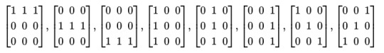
Find an element of V that is not in S.

Solution:

All these matrices have 2 corner 1s, so linear combinations will always have an even number of corner 1s. Hence a solution is

[onlinetrainingusa]

Python Libraries You Can't Ignore for Data Science

Recently, Python is the most widely used programming language. Developers are still in awe of its extraordinary powers to handle data science difficulties. Python's potential is already regularly utilized by many data scientists. Python has several positive qualities such as simplicity, debugging-friendliness, widespread use, object-oriented design, open-source nature, and excellent performance. 

Python provides many data science-specific libraries that programmers use regularly to solve challenging issues. Are you looking to become a professional Python developer to reach high in your career? If yes, take part in the best Python training online course to enrich your knowledge in Python libraries.

Here you can see the list of Python Libraries that are used for data science:

NumPy 

Numerous datasets can be managed, and array-based calculations can be carried out with the help of NumPy. This Python package made specifically for numerical computing. Its creators have used its powerful features to manage multi-dimensional arrays with great performance. NumPy matrices introduce vectorized arithmetic operations, boosting processing efficiency in contrast to Python's conventional looping techniques. 

A wide range of mathematical operations, such as addition, subtraction, multiplication, and division, are available in this adaptable library. NumPy interfaces without a hitch with other widely used data science libraries like pandas and Matplotlib, promoting unified workflows for data processing and visualization.

SciPy

A collection of mathematical algorithms and functions with the Python extension NumPy is called SciPy. This library belongs to the scientific community. For manipulating and displaying data, SciPy offers several high-level commands and classes. 

For data processing and system prototyping, SciPy is helpful. In addition to these benefits, SciPy offers many other complex, specialized applications that a strong and expanding Python programming community may support.

Keras 

The underlying frameworks TensorFlow, CNTK, or Theano are all compatible with Keras. It is a high-level neural network API for Python. Its major objective is to simplify speedy experimentation. The modularity, extensibility, and user-friendliness of Keras facilitate the development of deep learning models. 

Using short code snippets, Keras makes it simple to design, set up, and train neural networks. Layers, activation functions, loss functions, and optimizers are just a few of the commonly used neural network building pieces that are supported.

PyTorch 

PyTorch is an open-source machine learning framework for computer vision and natural language processing. It was created by the Facebook AI research team and is widely used in business and academia. You can easily transition from study to production due to PyTorch's dynamic computational graph. 

It also offers a flexible, approachable interface for creating and enhancing deep learning models. Also, PyTorch provides distributed processing, enabling speedy and effective model training on huge datasets.

Scikit-learn 

Scikit-learn are the most popular solution for resolving the problems with conventional machine learning. Approaches to learning that are supervised and unsupervised both make use of a wide range of algorithms. One of the benefits of the library is how simple it is to integrate other well-known packages on which it is built. 

Additional advantages include its vast community and thorough documentation. For research, industrial systems that use conventional techniques and beginners just getting started in this field, Scikit-learn is commonly employed. Scikit-learn do not resolve the loading, processing, manipulating, and visualizing issues. It is an expert in modeling both supervised and unsupervised learning techniques.

Pandas 

Developers need specific tools and procedures to evaluate and extract useful information from huge datasets. One of the libraries for data analysis that includes high-level data structures and easy-to-use tools for manipulating data is Pandas Python. 

It is necessary to be able to index, retrieve, split, join, restructure, and perform several other analyses on both multi- and single-dimensional data. It is to provide an easy-to-use but effective method of data analysis.

Final words

There are many other libraries in the Python ecosystem for handling advanced models and difficult operations. However, the Python libraries mentioned above are necessities for data science and are the foundation for additional, higher-level libraries. Enroll in the best Python training online course that covers important Python libraries, which add more value to your resume. 

Tags: Python, H2kinfosys, beginners for python, python programming learn, learn python language, python certification online, python online course certification, python training online, Top 10 Online Training Python in GA USA,Across the world high rating Online training for Python, world high rating Python course, World class python training, Live Online Software Training,100 percent job guarantee courses, vscode python,python programming language, python basic programs, python programming for beginners, freecodecamp python, learnpython, python code online,

 #onlinecertificatepython #beginnersforpython #pythonprogramminglearn #pythoncertificationonline, #pythononlinecoursecertification, #pythontrainingonline, #bestpythononlinetraining #Toptenonlinetrainingpython #PythonCourseOnline #PythonGAUSA, #H2KInfosys, #PythonCourse, #LearnPython, #PythonProgramming, #CodingWithPython, #PythonBasics, #PythonIntermediate #AdvancedPython, #c,#PythonForDataScience, #PythonForAI,#PythonWebDevelopment #PythonProjects

Contact:  +1-770-777-1269

Mail: training@h2kinfosys.com

Location - Atlanta, GA – USA, 5450 McGinnis Village Place, # 103 Alpharetta, GA 30005, USA.

Facebook: https://www.facebook.com/H2KInfosysLLC

Instagram: https://www.instagram.com/h2kinfosysllc/

Youtube: https://www.youtube.com/watch?v=p8cNzXQ6Nqk

Visit: https://www.h2kinfosys.com/courses/python-online-training/

Python Course: https://bit.ly/43SLdfk Visit for more info: H2kinfosys

[golzarrahman66-blog]

https://mathgr.com/grpost.php?grtid=1

ম্যাট্রিক্স কী?, ম্যাট্রিক্সের সারি ও কলাম কী?, ম্যাট্রিক্সের ক্রম কী?, ম্যাটিক্সের সাধারণ আকার কী?, ম্যাটিক্সের প্রকারভেদ কী?, সারি ম্যাট্রিক্স কী?, কলাম ম্যাট্রিক্স কী?, বর্গ ম্যাট্রিক্স কী?, ম্যাট্রিক্সের প্রধান কর্ণ কী?, উর্ধ ত্রিভুজাকার ম্যাট্রিক্স কী?, নিম্ন ত্রিভুজাকার ম্যাট্রিক্স কী?, কর্ণ ম্যাট্রিক্স কী?, স্কেলার ম্যাট্রিক্স কী?, একক বা অভেদক ম্যাট্রিক্স কী?, শুন্য ম্যাট্রিক্স কী?, সমঘাতি ম্যাট্রিক্স কী?, শুন্যঘাতি ম্যাট্রিক্স কী?, অভেদঘাতি ম্যাট্রিক্স কী?, বিম্ব ম্যাট্রিক্স কী?, প্রতিসম ম্যাট্রিক্স কী?, বিপ্রতিসম ম্যাট্রিক্স কী?, উপ-ম্যাট্রিক্স কী?, উল্লম্ব ম্যাট্রিক্স কী?, ম্যাট্রিক্সের ট্রেস কী?, পর্যায়বৃত্ত ম্যাট্রিক্স কী?, অনুবন্ধী ম্যাট্রিক্স কী?, হারমিসিয়ান ম্যাট্রিক্স কী?, বিহারমিসিয়ান ম্যাট্রিক্স কী?, ম্যাটিক্সের সমতা কী?, ম্যাটিক্সের যোগ কী?, ম্যাটিক্সের বিয়োগ কী?, ম্যাটিক্সের গুণ কী?, ম্যাট্রিক্সের স্কেলার গুণন কী?, ম্যাট্রিক্সের গুণন কী?, ম্যাট্রিক্সের গুণন যোগ্যতা কী?, Matrix, row and column of matrix, order of matrix, general form of matrix, types of matrix, row matrix, column matrix, square matrix, main diagonal of matrix, upper triangular matrix, lower triangular matrix, diagonal matrix, scalar matrix, singular or indistinguishable matrix, null matrix, Idempotent matrix, zero matrix, Transpose matrix, symmetric matrix, antisymmetric matrix, sub-matrix, vertical matrix, trace of matrix, periodic matrix, related matrix, Hermesian matrix, Bihermisian matrix, equality of matrices, addition of matrices, subtraction of matrices, multiplication of matrices, scalar multiplication of matrices, multiplication of matrices, Competence of multiplication of matrix

[skillslash]

Linear Algebra and Big Data: What You Need to Know

Linear Algebra is one of the most important mathematical concepts in big data and the data science world. It’s the basis for a bunch of different data processing and analysis methods, like machine learning, compression, and reducing dimensionality. 

In this article, we’re going to take a look at some of the most important concepts in Linear Algebra and how they apply to big data. 

What is Big Data? 

Big data is a huge and complex set of data that comes from all sorts of sources, like sensors, social networks, transactions, etc. It’s made up of three main parts: volume (the amount of data you have), speed (how fast you can generate it), and variety (the types of data you have). Big data analytics uses cutting-edge technologies and techniques like machine learning and data mining, as well as distributed computing to get valuable insights, patterns and trends from these data sets. This helps you make better decisions, streamline your business processes, and create new applications in different areas, like finance, healthcare, marketing, and more. 

Introduction to Linear Algebra 

Linear Algebra is a branch of math that looks at things like vectors and matrices and how they can be transformed. It’s a great way to solve linear equations, represent and manipulate data effectively, and understand complex relationships in different areas like physics, engineering, computers, and science. Some of the most important things to know about linear algebra are that you can think of it as an ordered list of scalars, and you can think of matrices as a rectangular array of numbers. All of these things have a lot of uses in data analysis and machine learning, as well as computer graphics, so linear algebra is really important for modeling and solving problems in real life. 

Let’s start by discussing some fundamental concepts : 

Vectors, Scalars and Matrices

Scalars are just numbers. Real numbers, integers, and even complex numbers can be used in data science to represent things like age or temperature 

Vectors, on the other hand, are lists of scalars that are ordered in size and direction. In big data, a vector can be used to represent any kind of data point or feature. 

Matrices are rectangular (scalar) arrays of numbers with rows and columns. They are used for storing and manipulating data. Matrices  are commonly used in big data to represent datasets, where each row represents an observation (for example, a person), and each column a different attribute (for example, age, income)

Matrix Operations

Matrix addition and subtractions can be done by adding or subtracting the same matrix of the same dimension. Scalar multiplication can be used to add or subtract the same matrix of different dimensions. 

Scalar multiplication multiplies each of the elements of a matrix by that particular scalar. Matrix Multiplication, also known as matrix dot product, is one of the basic operations of linear algebra. It is used when two matrices are multiplied, resulting in a new matrix.

Each of the elements in the matrix is a dot product of the row of the first row and the column of the second row. Matrix addition and subtraction are essential for many data transformations and for machine learning algorithms.

Applications of Linear Algebra in Big Data 

Now that we have a basic understanding of Big Data and linear algebra concepts, let’s explore how they are applied in the realm of big data: 

Data Representation 

Linear Algebra is a tool for the efficient representation and manipulation of data. In a large data environment, data is typically stored in the matrix form, where the rows represent observations and the columns represent characteristics. This representation facilitates the processing of large data sets. 

Dimensionality Reduction 

Big data often has a lot of features in it, which can cause the data to be too big or too small. This is known as the “curse of dimensionality”. Linear algebras, like Principal Component Analysis (PCA) and Singular Value Decomposition (SVD), can help reduce the size of the data while still keeping important information. This can help with visualization, modeling and even speeding up calculations. 

Machine Learning 

Machine learning algorithms often use linear algebra for model training and inference. For instance, linear regression relies on matrix multiplication to figure out the most accurate line for a set of data. Deep learning models also use a lot of matrix operations for forwards and backwards propagation. 

Eigenvalues and Eigenvectors 

Eigenvectors and Eigenvalues are really important when it comes to big data. They are used in a lot of different ways, like network analysis and recommendation systems, as well as image compression. Basically, Eigenvalues measure the amount of variation in the data, while Eigenvectors measure the direction of the maximum variance. 

Graph Analysis 

Graphs are used in big data analytics to represent the relationships between data points in a graph. Linear algebras, such as graph Laplacians and adjacency matrix, are used to analyze and extract information from large graphs, like social graphs or web page connections. 

Data Compression 

Singular Value Decomposition (SVD) and Principal Component Analysis (PCA), rely on linear algebra to represent data in a more compact form. This reduces storage requirements and speeds up data processing. 

Optimization Problems 

Linear Algebra is used to address optimization issues commonly encountered in machine learning and in data analysis. Algebraic techniques such as gradient descent involve the calculation of gradients, which represent vector operations, to determine the optimal model parameters. 

Natural Language Processing (NLP)

Linear algebra is used in Natural Language Processing (NLP) applications such as document grouping, topic modeling, or word embeddings to represent and analyze text data effectively. 

Signal Processing 

When it comes to signal processing, linear algebra is used in image and audio processing to do things like compress images, denoise them, and extract features. 

Quantitative Finance 

LinearAlgebra is one of the most important tools in finance when it comes to managing and analyzing big financial data. It’s used to optimize portfolios, assess risk, and price financial instruments. 

PageRank Algorithm 

The PageRank algorithm of Google, which assigns importance to web pages, is based on the principles of linear algebra. It is based on a directed graph model of the web and employs matrix operations to determine the importance scores associated with web pages, thus aiding in the ranking of search results.

12.    Image Compression 

Linear algebras can be utilized to reduce the size of large images while maintaining the essential data. This is essential for efficient image storage and transmission in applications such as video streaming and image distribution.. 

In summary, linear algebra is the fundamental mathematical structure that underlines many of the big data analytics (BDR) and data science approaches. Its flexibility and utility make it an indispensable tool for processing, understanding, and extracting value from large and intricate data sets. 

Conclusion

In conclusion, Linear Algebra is the foundation of Big Data Analytics and Data Science. Its broad concepts and operations are essential for transforming raw data into useful insights. From the representation of data in matrices and vectors, to the reduction of dimensionality, to the training of machine learning models, to the analysis of complex relationships in large charts, linear algebra is an essential tool for data professionals to meet the demands of the big data age. 

As the amount and complexity of data increases, it’s essential to have a good grasp of linear algebra. It helps data scientists and analysts quickly and effectively extract useful data from huge amounts of data. Plus, linear algebra gives us the theoretical basis for lots of advanced methods and algorithms, which can help us create breakthroughs in areas like AI, image processing, network analysis, and more.

[ankitcodinghub]

CSE131 - Homework #9 Solved

Objective : Learn how to use array and combine with for and while loops to implement some operations. 9.1 Write a program to use the rand() function to generate two twodimensional arrays of size 3*3, then output these matrices and implement addition, subtraction and multiplication operations. Hint: random between 0 ~ 100. Output: 9.2 Write a program let the user to input two numbers as the…

[gedthestudent]

The Last THAC0 Explanation

THAC0, short for “to-hit AC 0,” and descending armor class: a perennial example people enjoy using to explain why the editions of Dungeons & Dragons before the third are antiquated. There are many uncharitable descriptions of older editions of D&D and its retro-clones. The infamous THAC0, while unintuitive at first, is not convoluted. Here is the last THAC0 explanation anyone will ever need. Before there was Base Attack Bonus and ascending AC, there was THAC0 and descending AC. Before THAC0, there were attack matrices. For this example, we will establish that your edition or retro-clone of choice provides the entire attack matrix instead of just a character’s THAC0. Your character’s THAC0 would be the column of numbers under AC 0. Your attack rolls are as follows:

THAC0 - (sum of all attack modifiers) - 1d20 = descending AC “hit”

The game master calls for the attack roll, the player declares what descending AC they hit. The player hits the descending AC result and higher. You can reduce the math you have to do on a moment to moment basis by scratching down a modified THAC0 value. Remember to mind the parentheses. Therefore, the simplest attack roll is as follows:

Modified THAC0 - 1d20 = descending AC hit

Circumstantial modifiers that might improve or penalize your attack roll further then are subtracted or added to your THAC0, respectively. 

If you insist on converting everything to the ascending format, as per D&D 3e and beyond, then its a trivial matter. You convert THAC0 to Base Attack Bonus by subtracting THAC0 from 20. You convert descending AC to ascending AC by subtracting the descending AC from 20, or 19 if your game has an unarmored descending AC of 9. Again, mind the parentheses.

20 - THAC0 = BAB

20 - (descending AC) = ascending AC

You then arrive to attack roll resolution as most people understand it. 

1d20 + BAB = ascending AC hit

Circumstantial modifiers are added or subtracted from the roll as is. The ascending AC and lower is hit.

[pm-civil]

Addition & Subtraction of Matrices, Class 5th to 12th, Mathematics, @PMC...

Addition & Subtraction of Matrices, Class 5th to 12th, Mathematics, @PMCOACHINGCLASS Call 9527547380