#upper and lower bound theorem

[math-journal2]

<— Unit 21: Part 5 —>

Possible Zeros w/o calculator

*good to know but it’s impractical if you got 8 or 9 possible zeroes to eliminate. If possible, graphing calculator

Page 51

[experiment, ignore it]

Page 56

[bubbloquacious]

Zariski topologies

So if you take kⁿ, the n-dimensional coordinate space over some field k, the Zariski topology on kⁿ is the topology whose closed sets are of the form

Z(S) = { x ∈ kⁿ : f(x) = 0 for all f ∈ S }

for some subset S ⊆ k[x₁,...,xₙ]. That is, the closed sets are the common zero loci of some set of polynomials over k in n variables, i.e. they are the solution sets for some system of algebraic equations. Such sets are called algebraic sets. If I is the ideal generated by S, then Z(S) = Z(I), so we can restrict ourselves to ideals.

Now if you take a commutative unital ring R, we let Spec R denote its prime spectrum, the set of prime ideals of R. We let Max R ⊆ Spec R be the subset consisting of the maximal ideals, the maximal spectrum. The Zariski topology on Spec R is the topology whose closed sets are of the form

Z(S) = { P ∈ Spec R : P ⊇ S }

for some subset S ⊆ R. A prime ideal P contains S if and only if it contains the ideal generated by S, so again we can restrict to ideals. What's the common idea here? Classically, if k is algebraically closed, then Hilbert's Nullstellensatz (meaning Zero Locus Theorem) allows us to identify the points of kⁿ with those of Max k[x₁,...,xₙ], by mapping a point (a₁,...,aₙ) to the maximal ideal (x₁ - a₁,...,xₙ - aₙ), and the Zariski topologies will agree along this identification. There's nothing very special about these algebraic sets though.

Let X be any (pre-)ordered set with at least one bottom element. For a subset Y ⊆ X, define the lower and upper sets associated to Y as

L(Y) = { x ∈ X : x ≤ y for all y ∈ Y }, U(Y) = { x ∈ X : x ≥ y for all y ∈ Y }.

We call a lower [upper] set principal if it is of the form L(x)= L({x}) [U(x) = U({x})] for some x ∈ X. If X is complete (any subset has at least one least upper bound and greatest lower bound), then any lower or upper set is principal. Note that ⋂ᵢ L(Yᵢ) = L(⋃ᵢ Yᵢ), so lower sets are closed under arbitrary intersections; they provide what's called a closure system on the power set of X. The lower closure of a set Y is the intersection of all lower sets containing Y. We have that Y ⊆ L(x) if and only if x ∈ U(Y), so the lower closure of Y is given by L(U(Y)). If the lower sets were furthermore closed under finite unions (including empty unions), then they would form the closed sets of a topology on X.

This is not generally true; first of all, note that any lower set contains the bottom elements of X, of which there is at least one, so the empty set is not a lower set. As for binary unions, generally we have L(Y₁) ∪ L(Y₂) ⊆ L(Y₁ ∩ Y₂), but this inclusion might be strict. This is something we can fix by restricting to a subset of X.

We say that p ∈ X is prime if p is not a bottom element and for all x, y such that for all z such that x ≤ z and y ≤ z we have p ≤ z, we have that p ≤ x or p ≤ y. That is, if p is smaller than every upper bound of x and y, then p is smaller than x or y. Furthermore, we say that p is a prime atom if it is a minimal prime element. Let P(X) and A(X) denote the sets of primes and prime atoms of X, respectively. For a subset Y ⊆ X, let the Zariski closed set associated to Y be given by

Z(Y) = L(Y) ∩ P(X) = { p ∈ P(X) : p ≤ y for all y ∈ Y }.

We again have ⋂ᵢ Z(Yᵢ) = Z(⋃ᵢ Yᵢ), so the Zariski closed sets are closed under arbitrary intersections. Note also that Z(X) = ∅, so the empty set is closed. Now let Y₁, Y₂ be subsets of X. We find that Z(Y₁) ∪ Z(Y₂) = Z(U(Y₁ ∪ Y₂)). Clearly if p is smaller than all of the elements of one Yᵢ, then it is smaller than every upper bound; the interesting part is the other containment.

Assume that p ∈ Z(U(Y₁ ∪ Y₂)), so p is smaller than every upper bound of Y₁ ∪ Y₂. If p is smaller than every element of Y₁ then we are done, so assume that there is some y ∈ Y₁ with p ≰ y. For every y' ∈ Y₂ we have that p is smaller than every upper bound of y and y', so because p is prime we get that it is smaller than y or y'. It is not smaller than y, so p ≤ y'. We conclude that p ∈ Z(Y₂), and we're done.

As before, the Zariski closure of a set of primes Q ⊆ P(X) is given by Z(U(Q)). Note however that for a point x ∈ X we have L(x) = L(U(x)), so the Zariski closure of a prime p is Z(p). It follows that A(X) is exactly the subspace of closed points of P(X).

So we have defined the Zariski topology on P(X). How can we recover the classical examples?

If X is the collection of algebraic subsets of kⁿ ordered by inclusion, then P(X) consists of the irreducible algebraic subsets, and we can identify kⁿ itself with A(X). Our Zariski topology coincides with the standard definition.

If X = R is a unital commutative ring, ordered by divisibility, then being prime for the ordering coincides with being either prime for the ring structure, or being equal to 0 if R is an integral domain. Note that this ordering is not generally antisymmetric; consider 1 and -1 in a ring of characteristic not equal to 2.

A more well-behaved version of the previous example has X = { ideals I ⊴ R }, ordered by reverse inclusion. Note that for principal ideals (r), (s) we have (r) ⊇ (s) if and only if r divides s. We have P(X) = Spec R and A(X) = Max R, and our Zariski topology coincides with the standard definition.

You can play the same game if X is the lattice of subobjects of any structure H. If H is a set (or a topological space) and X is its power set, then the primes and prime atoms are the same; the points. The Zariski topology is the discrete topology on H. If H is a vector space, then P(X) is empty, because any non-zero subspace V can be contained in the span of two subspaces that don't contain V. It seems that the sweet spot for 'interesting' Zariski topologies is somewhere in between the rigidity of vector spaces and the flexibility of sets.

If H is an affine space, then again the prime elements are exactly the points. The resulting Zariski topology has as closed sets the finite unions of affine subspaces of H.

An interesting one is if X is the set of closed sets of some topological space S (generalizing the first example). The prime elements are the irreducible closed sets, and if S is T1 (meaning all points are closed), then the points of A(X) can be identified with those of S. Then the Zariski topology on A(X) is the same as the topology on S, and the Zariski closure of an irreducible closed set is the set of all irreducible closed sets contained in it.

[youzicha]

@argumate wrote:

complexity theory imposes various upper bounds on the size of problems you can solve, but I think the most important bounds are the lower bounds ones we’ve already established for many important problems: in cases where we already know the optimal algorithm then no AI can do any better regardless of how super intelligent it is.

now there are still a lot of suboptimal algorithms that can be improved, but the longer smart AI takes to show up the less there will be for it to do.

in the extreme case the final optimisation algorithm we discover will find nothing left to optimise.

I doubt it! I think hypothetically this could happen, but there are not many signs of it so far. As I see it (disclaimer here that I never seriously studied complexity theory), there’s a kind of qualitative difference between lower bounds for easy problems and for hard problems, and the AI stuff is hard.

For example, there are various famous algorithms for quickly finding shortest paths in graphs, which you could probably even invent yourself as a homework problem given some mild hinting. You may wonder if you “got it right”, and indeed, checking the literature there are various lower bounds for computing shortest paths, so if your algorithm matches the lower bound you are “done”.

After doing so, you might then think, “cool, now can I do the longest path problem too?” But no, the longest path problem is NP-hard, so even if you think for a really long time you’ll never get a fast algorithm. Instead you have to switch gear and e.g. consider additional properties that the inputs may have (like bounded treewidth), or pick a more heuristic algorithm like simulated annealing. (In the case when such an algorithm actually works, it probably also exploits some kind of additional property of the input, but it’s not too clear which one.) Here, the hardness result was useful not because it showed that your solution was correct, but because it indicated what “mode of thinking” you needed to be in to make progress.

If you were to get these two cases mixed up you’d reach some absurd conclusions. You can appeal to a hardness result saying that something will always need to take exponential time for some inputs, and then write a program that just does a brute-force search and claim that you have “solved” the problem. But if your program doesn’t run quickly enough, then that “solution” is useless. What the hardness really tells you is that the problem was poorly posed, and you can’t hope for something that works so generally.

And it seems when we think about “human level AI”, all the emblematic problems fall in the “hard” category. Theorem proving, planning, optimization, game playing, ... all of these are intractable in general. Of course, humans still try to muddle through, and so must the AI, but we know of no neat specification of these that we can solve optimally once and for all. It’s like that Conway quote: “Mathematics is the simple bit. It's the stuff we can understand. It's cats that are complicated.” We don’t even know where to start proving useful lower-bounds about cat-style problems!

[savrenim]

Hi so I'm studying optimization and I'm a bit stumped in regards to convexity. To be precise, I'm told that a problem has a unique minimum if both the function that will be minimised and the constraints are convex, but I can't see how a constraint (for example, (x^2)+(y^2)=3) can be convex, nor how that implies that the minimum is unique. Help?

Okay, woof, I would love to see a more specific wording of the problem because there are a couple of different things that are going on:

1. Every continuous function on a compact set (be it 1D, so a closed interval, or multidimensional--for example x^2+y^2=3 is the spherical shell of radius sqrt(3), which is both closed and bounded and hence compact but also a closed ball, rectangle, etc etc--note that this is compact, not convex, a convex set has a different meaning, although x^2+y^2=3 is convex too) reaches a global maximum and global minimum on that set. 

The proof of this is actually pretty clever: I'm going to go through the bullet points of the proof, feel free to ask me to comment more specifically on any of the bullet points if you want me to? but basically:

--a continuous function on a closed bounded set has a least upper bound and a greatest lower bound (it's defined everywhere, it's closed so there's no open-interval-can-tend-to-infinity-but-the-actually-asymptote-isn't-in-the-interval-so-we're-fine bit, so the values the function takes have to be bounded)--we'll do the least upper bound B, greatest lower is same argument. as it is the least upper bound, there have to be a sequence of x_n in the set such that f(x_n)>= B-1/n. this is basically stating that you can get arbitrarily close to the least upper bound, so why not pick a sequence of arbitrarily close points.--now the compact part is important: one of the definitions of a compact set, sequential compactness, is that every sequence has a convergent subsequence. so you can pick an x_(n_k) subsequence such that it converges to z for a point z in the set--and then by continuity, you can pass limits in and out of the function, so f(z)=f(lim k-->infty x_n_k)=lim_k-->infty f(x_n_k)=lim_k-->infty B-1/n_k=B.--so woohooo there exists at least one point which reaches THE GLOBAL maximum!

The two things that were necessary are indeed the weakest assumptions necessary; you NEED the function to be continuous for this to work, we used it in the proof to pass the limit inside the function, and you NEED the set to be compact for it to work; we used that to argue that the sequence had a convergent subsequence.

The problem with this is, this give existence, not uniqueness. So there will always be at least one point on a compact set with a continuous function that has a global maximum or minimum. BUT you could just as easily have two points that reach that value, or an infinite number of points. (technically any constant function on any compact set is continuous and does have a unique maximum/minimum value--its constant value--which it achieves literally everywhere on the set.)

So the place where boundary conditions come in is basically part 2: okay so what can we *also* say to go from there *exists* a point that achieves the max/min to it is a *unique* point that achieves the max/min. and uniqueness is really really hard to guarantee and so conditions get a lot more specific, and it turns out that one of the things that characterize convex functions the most is that they have under pretty loose conditions, unique minimums.

The basic idea as to why you want both the convex function and the convex set to be convex are, well, (and this is kind of oversimplifying it but I'd want to see the specific theorem you're talking about to be able to comment on exactly why the hypotheses of the theorem/what conditions your problem has to fulfill are what they are) -- but the basic idea is the math sees all the constraints involved very similarly? like if you're doing the Lagrange multiplier method (so we’re back to just continuous and compact set no guarantee of uniqueness) you have f that you're trying to minimize or maximize, and boundary conditions g, but the equations are grad(f)=lambda*grad(g), g=0 that are the system of equations that you solve, you're doing very very similar things to f and g. Well, a set is convex if and only if it is the area above the graph of a convex function. So requirements of a set to be convex/boundary conditions to be convex are because we will be using similar properties/procedures on all of the functions that we are looking at, be they the minimizable one or the boundary, so they better all follow the same rules. (but please, that is pretty touchy-feely instinct, send me the exact statement you want me to explain and I'll see if I can go through a proof of it if that's too vague for you)

If you want to get into more serious proofs, you start doing functional analysis. which means the fundamental theorem behind minimization is the geometric Hahn-Banach theorem and then it's basically convexity makes up for potential infinite dimensionality of your sets. which is fun. Hahn-Banach comes up E V E R Y W H E R E, it's a lifesaver

[craigbrownphd]

If you did not already know

Latent Profile Analysis (LPA) The main aim of LCA is to split seemingly heterogeneous data into subclasses of two or more homogeneous groups or classes. In contrast, LPA is a method that is conducted with continuously scaled data, the focus being on generating profiles of participants instead of testing a theoretical model in terms of a measurement model, path analytic model, or full structural model, as is the case, for example, with structural equation modeling. An example of LCA and LPA,is sustainable and active travel behaviors among commuters, separating the respondents into classes based on the facilitators of, and hindrances to, certain modes of travel. Quick Example of Latent Profile Analysis in R … nn-dependability-kit nn-dependability-kit is an open-source toolbox to support safety engineering of neural networks. The key functionality of nn-dependability-kit includes (a) novel dependability metrics for indicating sufficient elimination of uncertainties in the product life cycle, (b) formal reasoning engine for ensuring that the generalization does not lead to undesired behaviors, and (c) runtime monitoring for reasoning whether a decision of a neural network in operation time is supported by prior similarities in the training data. … Information Based Control (IBC) An information based method for solving stochastic control problems with partial observation has been proposed. First, the information-theoretic lower bounds of the cost function has been analysed. It has been shown, under rather weak assumptions, that reduction of the expected cost with closed-loop control compared to the best open-loop strategy is upper bounded by non-decreasing function of mutual information between control variables and the state trajectory. On the basis of this result, an \textit{Information Based Control} method has been developed. The main idea of the IBC consists in replacing the original control task by a sequence of control problems that are relatively easy to solve and such that information about the state of the system is actively generated. Two examples of the operation of the IBC are given. It has been shown that the IBC is able to find the optimal solution without using dynamic programming at least in these examples. Hence the computational complexity of the IBC is substantially smaller than complexity of dynamic programming, which is the main advantage of the proposed method. … Skipping Sampler We introduce the Skipping Sampler, a novel algorithm to efficiently sample from the restriction of an arbitrary probability density to an arbitrary measurable set. Such conditional densities can arise in the study of risk and reliability and are often of complex nature, for example having multiple isolated modes and non-convex or disconnected support. The sampler can be seen as an instance of the Metropolis-Hastings algorithm with a particular proposal structure, and we establish sufficient conditions under which the Strong Law of Large Numbers and the Central Limit Theorem hold. We give theoretical and numerical evidence of improved performance relative to the Random Walk Metropolis algorithm. … https://analytixon.com/2023/02/21/if-you-did-not-already-know-1972/?utm_source=dlvr.it&utm_medium=tumblr

[fennecfoxfavouritefox]

Algebraic number theory can prove the following cool theorem

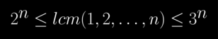
For large n. (n > 6)

Here are proofs for the lower bound and the upper bound

[watchergreys]

Format papier de infix pro

#Format papier de infix pro series

final section we indicate, by means of an example, how the method of producing lexicodes can be applied optimally to find anncodes. We also give a short proof of the basic properties of the previously known lexicodes, which are defined by means of an exponential algorithm, and are related to game theory. We show that annihilation games provide a potentially polynomial method for computing codes (anncodes). The "losing positions" of certain combinatorial games constitute linear error detecting and correcting codes. We also study whether the fixed-point operator preserves prefix closure, relative closure (also called Lm(G)-closure), and controllability. Fixed-point based characterization of all the above language classes is also given, and their closure under intersection/union is investigated. The computation of super/sublanguages and also computation of their upper/lower bounds has lead to the introduction of other classes of co-observable languages, namely, strongly C&P co-observable languages, strongly D&A co-observable languages, locally observable languages, and strongly locally observable languages. the class of co-observable languages is not closed under intersection/union, we provide upper/lower bound of the super/sublanguage formula we present. We also provide formulas for computing super/sublanguages for each of these classes. We present fixed-point based characterization of several classes of co-observable languages that are of interest in the context of decentralized supervisory control of discrete-event systems, including C&P ∨ D&A co-observable languages, C&P co-observable languages, and D&A co-observable languages.

#Format papier de infix pro series

These notes for a series of lectures at the VI-th SERC Numerical Analysis Summer School, Leicester University, apply the principles of validated computatio. In contrast, validated computation ffl checks that the hypotheses of appropriate existence and uniqueness theorems are satisfied, ffl uses interval arithmetic with directed rounding to capture truncation and rounding errors in computation, and ffl organizes the computations to obtain as tight an enclosure of the answer as possible. analysis to help provide this insight, but even the best codes for computing approximate answers can be fooled. One key insight we wish from nearly all computing in engineering and scientific applications is, "How accurate is the answer?" Standard numerical analysis has developed techniques of forward and backward error. Hamming once said, "The purpose of computing is insight, not numbers." If that is so, then the speed of our computers should be measured in insights per year, not operations per second.

[arxt1]

Lower bound for the neutrino magnetic moment from kick velocities induced at the birth of neutron stars. (arXiv:1912.10294v2 [astro-ph.HE] UPDATED)

We show that the neutrino chirality flip, that can take place in the core of a neutron star at birth, is an efficient process to allow neutrinos to anisotropically escape, thus providing a to induce the neutron star kick velocities. The process is not subject to the {\it no-go theorem} since although the flip from left- to right-handed neutrinos happens at equilibrium, the reverse process does not take place given that right-handed neutrinos do not interact with matter and therefore detailed balance is lost. For simplicity, we model the neutron star core as being made of strange quark matter. We find that the process is efficient when the neutrino magnetic moment is not smaller than $4.7 \times 10^{-15}\mu_B$, where $\mu_B$ is the Bohr magneton. When this lower bound is combined with the most stringent upper bound, that uses the luminosity data obtained from the analysis of SN 1987A, our results set a range for the neutrino magnetic moment given by $4.7 \times 10^{-15} \leq \mu_\nu/\mu_B \leq (0.1 - 0.4)\times 10^{-11}$. The obtained kick velocities for natal conditions are consistent with the observed ones and span the correct range of radii for typical magnetic field intensities.

from astro-ph.HE updates on arXiv.org https://ift.tt/396Ajq9

[wayneradinsky]

'A statistician teaches deep learning'. He says, 'Statisticians have different training and instincts than computer scientists.' OMG is that so true. I realized that when I first tried to use the R programming language. R is a programming language made by and for statisticians, not computer scientists. I wish I had made a list of all the weird things about it (which I can't remember any more because I don't use it on a regular basis and probably won't as more and more of its functionality is being replicated in the Python world), as it is one of the whackiest programming languages in the world. I guess my mind is more "computer sciency"; statisticians seem twisted to me. Which is not to say I'm not going to learn more statistics (always have to learn more statistics).

Anyway, so, what does this statistician say the differences between statisticians and computer scientists are? Well, not computer scientists in general; he focuses on "deep learning computer scientists". He says:

"One contrast between statisticians and deep learning computer scientists is that we generally make predictions and classifications using linear combinations of basis elements -- this is the cornerstone of nearly all regression and much classification, including support vector machines, boosting, bagging, and stacking (nearest-neighbor methods are a rare exception). But deep learning uses compositions of activation functions of weighted linear combinations of inputs. Function composition enables one to train the network through the chain rule for derivatives, which is the heart of the backpropagation algorithm."

"The statistical approach generally enables more interpretability, but function composition increases the space of models that can be fit. If the activation functions in the deep learning networks were linear, then deep learning in a regression application would be equivalent to multiple linear regression, and deep learning in a classification application would be equivalent to linear discriminant analysis. In that same spirit, a deep variational autoencoder with one hidden layer and linear activation functions is equivalent to principal components analysis. But use of nonlinear activation functions enables much more flexible models. Statisticians are taught to be wary of highly flexible models."

I'm going to assume you all don't want to download the paper (19-page PDF) with equations so I'm going to continue on and pull out some more choice quotes.

"Statisticians worry about overparameterization and issues related to the Curse of Dimensionality. But deep learning frequently has millions of parameters. Even though deep learning typically trains on very large datasets, their size still cannot provide sufficient information to overcome the Curse of Dimensionality. Statisticians often try to address overparameterization through variable selection, removing terms that do not contribute significantly to the inference. This generally improves interpretability, but often makes relatively strong use of modeling assumptions. In contrast, deep learning wants all the nodes in the network to contribute only slightly to the final output, and uses dropout (and other methods) to ensure that result. Part of the justification for that is a biological metaphor -- genome-wide association studies find that most traits are controlled by many, many genes, each of which has only small effect."

"And, of course, with the exception of Chen et al., deep learning typically is not concerned with interpretability, which is generally defined as the ability to identify the reason that a particular input leads to a specific output. deep learning does devote some attention to explainability, which concerns the extent to which the parameters in deep networks can shape the output. To statisticians, this is rather like assessing variable importance.

"Statistics has its roots in mathematics, so theory has primacy in our community. Computer science comes from more of a laboratory science tradition, so the emphasis is upon performance. This is not say that there is no theory behind deep learning; it is being built out swiftly. But much of it is done after some technique has been found to work, rather than as a guide to discovering new methodology. One of the major theorems in deep learning concerns the universal approximation property."

"One of the most important theoretical results for deep learning are upper bounds on its generalization error (also known as expected loss). Such bounds indicate how accurately deep learning is able to predict outcomes for previously unseen data. Sometimes the bounds are unhelpfully large, but in other cases they are usefully small."

"In statistics, we worry about the bias-variance tradeoff, and know that overtraining causes performance on the test sample to deteriorate after a certain point, so the error rate on the test data is U-shaped as a function of the amount of training. But in deep learning, there is a double descent curve; the test error decreases, rises, then decreases again, possibly finding a lower minimum before increasing again. This is thought to be because the deep learning network is learning to interpolate the data. The double descent phenomenon is one of the most striking results in modern deep learning research in recent years. It occurs in CNNs, ResNets, and transformers."

"Deep learning models are often viewed as deterministic functions, which limits use in many applications. First, model uncertainty cannot be assessed; statisticians know this can lead to poor prediction. Second, most network architectures are designed through trial and error, or are based upon high level abstractions. Thus, the process of finding an optimal network architecture for the task at hand, given the training data, can be cumbersome. Third, deep models have many parameters and thus require huge amounts of training data. Such data are not always available, and so deep models are often hampered by overfitting. Potentially, these issues could be addressed using Bayesian statistics for uncertainty quantification."

"It is important to recognize that deep learning can fail badly. In particular, deep learning networks can be blindsided by small, imperceptible perturbations in the inputs, also known as data poisoning. The attackers need not even know the details of the machine learning model used by defenders.

"One important case is autonomous vehicles, where deep learning networks decide, e.g., whether the latest sequence of images implies that the car should apply its brakes. There are now many famous cases in which changing a few pixels in training data can creates holes in deep learning network performance. Symmetrically, a small perturbation of an image, such as applying a post-it note to a stop sign, can fool the deep learning network into classifying it has a billboard and not recognizing that the vehicle should brake."

I skipped a few things like Kullback-Leibler divergence reversal, which pertains to how a statistician would look at generative adversarial networks (GANs), which are the neural networks that generate fake things, like images of people that don't exist. But that section was pretty much all equations. He goes on to outline a curriculum that he thinks would be ideal for statisticians who want to learn deep learning.

[ijtsrd]

A Note on the Generalization of the Mean Value Theorem

by Yeong-Jeu Sun "A Note on the Generalization of the Mean Value Theorem"

Published in International Journal of Trend in Scientific Research and Development (ijtsrd), ISSN: 2456-6470, Volume-5 | Issue-1 , December 2020,

URL: https://www.ijtsrd.com/papers/ijtsrd38258.pdf

Paper URL : https://www.ijtsrd.com/mathemetics/calculus/38258/a-note-on-the-generalization-of-the-mean-value-theorem/yeongjeu-sun

callforpapermedicalscience, medicalsciencejournal, manuscriptsubmission

In this paper, a new generalization of the mean value theorem is firstly established. Based on the Rolle’s theorem, a simple proof is provided to guarantee the correctness of such a generalization. Some corollaries are evidently obtained by the main result. It will be shown that the mean value theorem, the Cauchy’s mean value theorem, and the mean value theorem for integrals are the special cases of such a generalized form. We can simultaneously obtain the upper and lower bounds of certain integral formulas and verify inequalities by using the main theorems. Finally, two examples are offered to illustrate the feasibility and effectiveness of the obtained results. 

[math-journal2]

<— Unit 21: Part 4 —>

Possible Zeros 2

*assuming you DO NOT have a graphing calculator, only scientific

Descartes Rule of Signs

#1

Upper & Lower Bounds

Theorem

#1

Overall Strategy

Page 55

[kubleeka]

Constructing the Real Numbers III

The real numbers form a unique, complete ordered field.

I’ve already discussed general fields and ordered fields in the previous posts. Here, we’ll discuss completeness. This part is long enough that I’m splitting it across two posts, but when we’ve finished with it, our construction will be done.

Completeness

The statement that an ordered field is complete can be formalized in a lot of different-looking ways. Intuitively, we can think of it as “filling in the gaps” in incomplete fields like the rational numbers. Saying that the real numbers are complete means that every sequence that is increasing and bounded above converges, that every decimal expansion actually refers to a real number, and allows intuitive results like the Intermediate Value Theorem to hold.

We start with the most standard version of the completeness axiom:

The Completeness Axiom: If \(\mathbb{R}\) is an ordered field, then every nonempty subset of \(\mathbb{R}\) with an upper bound has a least upper bound.

Let’s break that down: an upper bound of a set is just a number that’s greater than or equal to every member of the set. So if our set is the set of reciprocals of natural numbers, \(\{\frac{1}{n} | n\in\mathbb{N}\}\), then \(1\), \(7\), and \(193.5\) are all upper bounds of the set. Note that an upper bound does not have to actually belong to the set.

Then, naturally, the least upper bound is the upper bound that is smaller than every other upper bound. The least upper bound of a set \(S\) is also called the supremum (plural suprema) of \(S\), or \(\sup S\). It’s clear now that suprema are unique as well: if there were two distinct suprema of a set, one must be larger than the other, and then it’s not a least upper bound.

We can also define and prove the existence of an infimum (plural infima), or greatest lower bound for every set with some lower bound, as an exercise. (Hint: for a set \(S\) with a lower bound, consider the set of numbers less than every element of \(S\) ).

Now, we need the notion of a sequence. We can think of a sequence as an infinite, ordered list of real numbers. More formally, it’s a function from the natural numbers to the reals, so every natural number gets associated with an element. If the name of our sequence is \(\{a_n\}\), we write it as \(\{a_n\}=\{a_1, a_2, a_3 \dots\}\). Note that \(\{a_n\}\) refers to the sequence itself, while \(a_n\) (no brackets) refers to the \(n\)th term of the sequence.

Some sequences seem to approach a certain value as we look further and further along them. For example, the terms of the sequence \(\{\frac{1}{n}\}\) approach \(0\). That is, for any given margin of error \(\varepsilon\), if we just look far enough down the sequence, we can find a point where every term of the sequence is within \(\varepsilon\) of \(0\).

To demonstrate this definition, let’s prove rigorously that \(\{\frac{1}{n}\}\) converges to \(0\). We want the sequence to get within \(\varepsilon\) of \(0\), for any given \(\varepsilon>0\). That is, we want \(|\frac{1}{n}-0|=\frac{1}{n}<\varepsilon\).

Now, choose \(M\) such that \(M>\frac{1}{\varepsilon}\). Then for every \(n>M\), we have \(n>M>\frac{1}{\varepsilon}\). So \(n>\frac{1}{\varepsilon}\), so \(\frac{1}{n}<\varepsilon\) as desired.

So, having produced a formula for choosing \(M\) in terms of \(\varepsilon\), the proof is complete, and the limit of \(\{\frac{1}{n}\}\) is \(0\).

You can make a career out of studying sequences of real numbers like this, but here are some important highlights:

Limits are Unique: Suppose a sequence converged to two different numbers, \(A\) and \(B\). Since \(A\) is a limit, there must be a point where for any error margin \(\varepsilon\), the sequence gets (and remains) within \(\varepsilon\) of \(A\). Let \(\varepsilon<|B-A|\), and note that the sequence is now limited in how close it can get to \(B\). So \(B\) is not, in fact, a limit.

Monotone Convergence Theorem: If a sequence \(\{x_n\}\) is strictly increasing and bounded above, or strictly decreasing and bounded below, then it converges. Moreover, it converges to the least upper bound or greatest lower bound.

Proof sketch: This is a fairly intuitive result. We can find a point in the sequence where every subsequent term is within \(\varepsilon\) of the supremum. There must be at least one term between \(\sup \{x_n\}\) and \(\sup \{x_n\}-\varepsilon\). For if there wasn’t, we would have an improved lower bound of \(\sup \{x_n\}-\varepsilon\). Then every subsequent term must be greater that \(\sup \{x_n\}-\varepsilon\), since the sequence is increasing. And every subsequent term must be less than \(\sup \{x_n\}\), since that’s an upper bound. QED (The proof for the decreasing/bounded below case is analogous.)

Remember: the reason this is an important result is that the limit of the sequence must itself be a real number (thanks to completeness). So we can actually use convergent sequences to pinpoint particular real numbers (thanks to uniqueness of limits).

Now, we’ll define a special type of sequence, called a series. We can define a series naturally given any sequence. If the sequence is \(\{a_n\}\), then the series is denoted \(\sum a_n\), and is the sequence \(\{a_1, a_1+a_2, a_1+a_2+a_3, …\}\). The \(n\)th term of the series is the sum of the first \(n\) terms of \(a_n\). Note that if \(\{a_n\}\) is strictly positive, then \(\sum a_n\) is strictly increasing.

We say a series is geometric when its defining sequence is of the form \(\{a_n\}=\{a, ar, ar^2, ar^3, \dots\}\) for some real numbers \(a\) and \(r\).

Theorem: If \(0<r<1\), then \(\sum ar^n\) converges.

Suppose \(a>0\). Then every term of \(\{ar^n\}\) is positive, so \(\sum ar^n\) is a strictly increasing sequence. Now, by Monotone Convergence Theorem, it’s sufficient to show that \(\sum ar^n\) is bounded above.

Claim: \(\sum ar^n\) is bounded above by \(\frac{a}{1-r}\).

Suppose for some \(k\), \(a+ar+\dots+ar^k>\frac{a}{1-r}\). Now consider the number \(a-ar^{k+1}\). Clearly, this number is less than \(a\); we start with \(a\), then subtract a positive number.

But \(a-ar^{k+1}\) can be factored as \((1-r)(a+ar+\dots+ar^k)\), and

\((1-r)(a+ar+\dots+ar^k)>(1-r)\frac{a}{1-r}=a\). So \(a-ar^{k+1}>a\), a contradiction.

So there can be no \(k\) where \(a+ar+\dots+ar^k>\frac{a}{1-r}\), and so the series is bounded above. QED

If \(a<0\), then \(\sum a_n\) is strictly decreasing, and the argument is identical to the one above, just with the signs flipped.

(Exercise: show that the series converges to \(\frac{a}{1-r}\) exactly.)

We’re 90% of the way to building decimal notation. We’ll finish it in the next post, then use it to show something very weird about the reals.

[mathematicianadda]

Geometric Similarity of Functions https://ift.tt/3jnkPC3

I am a 16 year old high school student and recently I have written a paper on a numerical approximation of distinct functions. I have shown my teachers this and they do not understand it. My questions: Is this a valid theorem to use to estimate functions with differently based functions? Has something similar already been created? Is it all useful/publishable? Any tips on how to improve? I will give an outline but you can find it here: https://www.overleaf.com/read/xjqhfgvrcrbj

Definitions

Geometric similarity refers to the dilation of a particular shape in all its dimensions. Proofs of geometric similarity are included in congruence proofs of triangles with AAA (Angle-Angle-Angle) proofs. Knowing the sizes of all sides of both triangles: $\triangle{ABC}$ and $\triangle{A'B'C'}$, to find the dilation factor and prove geometric similarity the following must be true: $\frac{\mid A' \mid}{\mid A \mid} =\frac{\mid B' \mid}{\mid B \mid}=\frac{\mid C' \mid}{\mid C \mid}$.

Interpreting functions as shapes on the Cartesian plane and using geometry, geometrically similar functions can be calculated. Analytically this would imply for a function $y=f(x)\; \{x_0\leq x \leq x_1\}$ a geometrically similar function would be of the form $ny=f(nx)\;\{\frac{x_0}{n}\leq x \leq \frac{x_1}{n}\}$ where $n\in {\rm I\!R}$. This is because the function is scaled by the same factor in the $x$ and $y$ direction thus would be geometrically similar.

$y_1=\sin(x)\;\{0\leq x \leq 2\pi\}$ and $y_2=\frac{1}{2}\sin(2x)\; \{0 \leq x\leq \pi\}$" />

However to compare two functions which are distinct, multiplying $x$ and $y$ by $n$ will not suffice for proving similarity. The formula to find the dilation factor can be used to prove similarity between two functions. By describing a function geometrically it has three superficial 'edges' which can be represented as sets. Two of the edges are the two axis $x$ and $y$. The length of the side '$y$' is the $\max \{ f(x) : x = 1 .. n \}-\min \{ f(x) : x = 1 .. n \}$ and the length of the side $x$ is $b_1$-$a_1$ where $b_1$ is the upper bound and $a_1$ is the lower bound. Finally the third side of the function will be the arc length over the interval $\{a_1\leq x\leq b_1\}$. Another characteristic for two shapes to be geometrically similar is the area is increased by the dilation factor squared.Thus from the formula for the dilation factor for two similar triangles the following theorem can be derived:

Theorem Let $y_1\;\{a_1\leq x \leq b_1\}$ and $y_2\;\{a_2\leq x \leq b_2\}$ be functions whose derivative exists in every point. If both functions are geometrically similar then the following system holds: \begin{equation} \frac{1}{\big(b_1-a_1\big)}\int_{a_1}^{b_1} \sqrt{1+\bigg( \frac{dy_1}{dx} \bigg) ^{2} } dx= \frac{ 1 }{ \big(b_2-a_2\big) } \int_{a_2}^{b_2} \sqrt{1+\bigg( \frac{dy_2}{dx} \bigg) ^{2} } dx \end{equation} \begin{equation} \frac{1}{\big(b_1-a_1\big)^2} \int_{a_1}^{b_1} y_1 dx= \frac{1}{\big(b_2-a_2\big)^2}\int_{a_2}^{b_2} y_2dx \end{equation}

Similarity Between Distinct Functions

When describing a function as distinct it denotes that the functions have different bases, i.e. sinusoidal and exponential. As mentioned above, for geometric similarity to exist of a function $y=f(x)$ the resultant function will become $ny=f(nx)$. However if comparing functions of different bases, equations (1) and (2) are necessary to find the bounds of similarity. For example, the problem:

Find the bounds $b$ and $a$ where $e^x\;\{0\leq x\leq 1\}$ is similar to $x^2 $.

To see examples go to the above link. Any help would be much appreciated and apologies if this is crude mathematics.

from Hot Weekly Questions - Mathematics Stack Exchange hwood87 from Blogger https://ift.tt/2FYTbOm

[craigbrownphd-blog-blog]

If you did not already know

AIOps AIOps platforms utilize big data, modern machine learning and other advanced analytics technologies to directly and indirectly enhance IT operations (monitoring, automation and service desk) functions with proactive, personal and dynamic insight. AIOps platforms enable the concurrent use of multiple data sources, data collection methods, analytical (real-time and deep) technologies, and presentation technologies. … Unicorn Some real-world domains are best characterized as a single task, but for others this perspective is limiting. Instead, some tasks continually grow in complexity, in tandem with the agent’s competence. In continual learning, also referred to as lifelong learning, there are no explicit task boundaries or curricula. As learning agents have become more powerful, continual learning remains one of the frontiers that has resisted quick progress. To test continual learning capabilities we consider a challenging 3D domain with an implicit sequence of tasks and sparse rewards. We propose a novel agent architecture called Unicorn, which demonstrates strong continual learning and outperforms several baseline agents on the proposed domain. The agent achieves this by jointly representing and learning multiple policies efficiently, using a parallel off-policy learning setup. … Robust Stochastic Optimization (DRO) A common goal in statistics and machine learning is to learn models that can perform well against distributional shifts, such as latent heterogeneous subpopulations, unknown covariate shifts, or unmodeled temporal effects. We develop and analyze a distributionally robust stochastic optimization (DRO) framework that learns a model that provides good performance against perturbations to the data-generating distribution. We give a convex optimization formulation for the problem, providing several convergence guarantees. We prove finite-sample minimax upper and lower bounds, showing that distributinoal robustness sometimes comes at a cost in convergence rates. We give limit theorems for the learned parameters, where we fully specify the limiting distribution so that confidence intervals can be computed. On real tasks including generalizing to unknown subpopulations, fine-grained recognition, and providing good tail performance, the distributionally robust approach often exhibits improved performance. … Dynamic Distributed Dimensional Data Model (D4M) A crucial element of large web companies is their ability to collect and analyze massive amounts of data. Tuple store databases are a key enabling technology employed by many of these companies (e.g., Google Big Table and Amazon Dynamo). Tuple stores are highly scalable and run on commodity clusters, but lack interfaces to support efficient development of mathematically based analytics. D4M (Dynamic Distributed Dimensional Data Model) has been developed to provide a mathematically rich interface to tuple stores (and structured query language ‘SQL’ databases). D4M allows linear algebra to be readily applied to databases. Using D4M, it is possible to create composable analytics with significantly less effort than using traditional approaches. This work describes the D4M technology and its application and performance. … https://bit.ly/2WiwIzI

[thousandmaths]

The Total Acquisition Number of a Randomly Weighted Path

This talk was given by Elizabeth Kelley at our student combinatorics seminar. She cited Godbole, Kurtz, Pralat, and Zhang as collaborators. One of these (Pralat, I think) was originally an editor, but then made substantial contributions to the project. This post is intended to be elementary.

[ Personal note: This is the last talk post I will be writing for OTAM. It seems fitting, since Elizabeth and I went to the same undergrad; I have actually known her for almost as long as I have been doing mathematics. ]

------

Acquisitions Incorporated

This is a graph theory talk, but, refreshingly, it did not begin with “A graph is a pair of vertices and edges such that...”

It did begin with this: Let $G$ be a graph with a vertex-weighting (i.e. an assignment of nonnegative reals to each vertex). An acquisition move is a “complete transfer of weight” from a low-weight vertex to an adjacent higher-weight vertex. In other words, if the weights before the move are $w\leq x$, then the weights after the move are $0\leq w+x$ (respectively).

[ For the sake of not cluttering up the definitions with trivialities, we will say that both of the weights involved in an acquisition move must be strictly positive— that is: not zero. ]

From this, a bunch of definitions follow in quick succession. 

A sequence of acquisition moves is called an acquisition protocol if it is maximal, i.e. after performing all of the moves, no further move is possible.

The set of nonzero-weight vertices after performing an acquisition protocol is called a residual set.

Finally, the acquisition number of $G$ is the minimum size of any residual set. We write it as $a(G)$.

This explains half of the title. The other half of the title, is perhaps a bit more self-explanatory. A lot is known about acquisition numbers when, say, all vertices are given weight $1$. Less is known in other contexts, but the goal of this paper is to ask what we “should” expect for paths. More precisely: if we give the vertices random weights, what is the expected acquisition number?

------

Fekete’s Lemma

A sequence of real numbers $(x_n)$ is called subadditive if it does what the name suggests: for all $n$ and $m$

$$ x_{n+m} \leq x_n + x_m.$$

This is a pretty general construction, and tons of sequences do this: certainly any decreasing sequence will, and also most reasonable sequences that grow slower than linear ($\log(n)$ works, for instance). Usually, when the situation is so general, it is hard to say anything at all about them, but in this case things are different:

Lemma (Fekete). Given any subadditive sequence $(x_n)$, the limit of $x_n/n$ exists, and moreover

$$ \lim_{n\to\infty} \frac{x_n}{n} = \text{inf}_n \frac{x_n}{n}. $$

(This lemma has one of my favorite proofs, which is essentially the same as the one given in this NOTSB post; just reverse all the inequalities and repeat the argument with liminf/limsup replaced by lim/inf.)

This means that whenever you have a subadditive sequence, it makes sense to ask about its growth rate, which is just the limit that Fekete guarantees exists. Less formally, it is the number $c$ such that $x_n \approx cn$ as $n$ gets large. (Perhaps in this formulation is the existence statement so striking: why should there be such a number at all? But Fekete states that there is.)

As it happens, it is pretty easy to prove that $a(P_n)$, where the path $P_n$ on $n$ vertices has been weighted with all 1s, forms a subadditive sequence.

This proof doesn’t use much about the weightings at all: it requires only that they are “consistent” in some technical sense. The punchline for our purposes is that $a(P_n)$ continues to form a subadditive sequence when the paths are weighted by independent identically distributed random variables.

------

Numbers, Please!

In the paper, Kelley considered the case when the vertex weights were distributed as a Poisson distribution. This is a thing whose details aren’t too important, but if you’re familiar with it you may be wondering why this instead of anything else? The answer is because when you know the answer for the Poisson model, you also know it in a more physically reasonable model: you start with a fixed amount of weight and you distribute it randomly to the vertices.

[ The process by which you use Poisson to understand the latter model is called “dePoissonization”, which makes me smile: to me it brings to mind images of someone hunched over their counter trying to scrub the fish smell out of it. ]

But enough justification: what’s the answer? Well, we don’t actually know the number on the nose, but here’s a good first step:

Theorem (Godbole–Kelley–Kurtz–Pralat–Zhang). Let the vertices of $P_n$ be weighted by Poisson random variables of mean $1$. Then $0.242n \leq \Bbb E[a(P_n)] \leq 0.375n$.

The proof of this theorem is mostly number-crunching, except for one crucial insight for each inequality: This step is easier to prove for the lower bound: after we have assigned numbers for the random variables, check which functions have been given the weight zero and look at the “islands” between them. Acquisition moves cannot make these islands interact, and so we can deal with them separately, so $\Bbb E[a(P_n)]$ splits up into a sum of smaller expectations based on the size of the islands. In a strong sense “most” of the islands will be small, and so you get a pretty good approximation just by calculating the first couple terms.

To get an upper bound, you need to think of strategies which will work no matter low long the path is and what variables are used. The most naïve strategy is to just pair off vertices of the path and send the smaller one in the pair to the larger one. This may or may not be an acquisition protocol, but you will always cut the residual set size (roughly) in half. Following even this naïve strategy is good enough to give the 0.375.

Both of these steps are fairly conceptually straightforward, but it becomes very difficult to calculate all the possibilities as you get further into the sum; in other words, it’s a perfect problem for looking to computer assistance. This allows us to get theoretical bounds $0.29523n \leq \Bbb E[a(P_n)] \leq 0.29576n$; and of course it would not be hard to get better results by computing more terms, but at some point it’s wiser to start looking for sharper theoretical tools rather than just trying to throw more computing power toward increasingly minuscule improvements.

[juniperpublishers-robotics-blog]

Differential Evolution (DE): A Short Review- Juniper Publishers

Abstract

Proposing new mutation strategies and adjusting control parameters to improve the optimization performance of differential evolution (DE) are considered a vital research study. Therefore, in this paper, a short review of the most significant contributions on parameter adaptation and developed mutation strategies is presented.

Keywords: Evolutionary computation; Global optimization; Differential evolution; Mutation strategy; Adaptive parameter control

Abbreviations: DE: Differential Evolution; EAs: Evolutionary Algorithms; CR: Crossover Rate; SF: Scaling Factor; FADE: Fuzzy Adaptive Differential Evolution; SDE: Self Adaptive Differential Evolution

Introduction

Differential Evolution (DE), proposed by Storn and Price [1,2] is a stochastic population-based search method. It exhibits excellent capability in solving a wide range of optimization problems with different characteristics from several fields and many real-world application problems [3]. Similar to all other Evolutionary algorithms (EAs), the evolutionary process of DE uses mutations, crossover and selection operators at each generation to reach the global optimum. Besides, it is one of the most efficient evolutionary algorithms (EAs) currently in use. In DE, each individual in the population is called target vector. Mutation is used to generate a mutant vector, which perturbs a target vector using the difference vector of other individuals in the population. After that, crossover operation generates the trial vector by combining the parameters of the mutation vector with the parameters of a parent vector selected from the population. Finally, according to the fitness value and selection operation determines which of the vectors should be chosen for the next generation by implementing a one-to-one completion between the generated trail vectors and the corresponding parent vectors [4,5]. The performance of DE basically depends on the mutation strategy, the crossover operator. Besides, The intrinsic control parameters (population size NP, scaling factor F, the crossover rate CR) play a vital role in balancing the diversity of population and convergence speed of the algorithm. The advantages are simplicity of implementation, reliable, speed and robustness [3]. Thus, it has been widely applied in solving many real-world applications of science and engineering, such as {0-1} Knapsack Problem [6], financial markets dynamic modeling [7], feature selection [8], admission capacity planning higher education [9,10] , and solar energy [11], for more applications, interested readers can refer to [12]. However, DE has many weaknesses, as all other evolutionary search techniques do w.r.t the NFL theorem. Generally, DE has a good global exploration ability that can reach the region of global optimum, but it is slow at exploitation of the solution [13]. Additionally, the parameters of DE are problem dependent and it is difficult to adjust them for different problems. Moreover, DE performance decreases as search space dimensionality increases [14]. Finally, the performance of DE deteriorates significantly when the problems of premature convergence and/or stagnation occur [14,15]. Consequently, researchers have suggested many techniques to improve the basic DE. From the literature [12,16,17], these proposed modifications, improvements and developments on DE focus  on adjusting control parameters in an adaptive or self-adaptive manner while there are a few attempts in developing new mutations rule.

Differential Evolution

This section provides a brief summary of the basic Differential Evolution (DE) algorithm. In simple DE, generally known as DE/rand/1/bin [2,18], an initial random population, denoted by P, consists of NP individual. Each individual is represented by the vector, = (x1,i,x2,ixD,i) where D is the number of dimensions in solution space. Since the population will be varied with the running of evolutionary process, the generation times in DE are expressed by G = 0,I,...,Gmax , where is the maximal time of generations. For the ith individual of P at the G generation, it is denoted by xGi = (xG1,i, xG2,i,..., xGD,i) . The lower and upper bounds in each dimension of search space are respectively recorded by xL = (x1,L, x2,L,..., xD,L) and xu = (xl, u, x2,u,..., xD,u ). The initial population P0is randomly generated according to a uniform distribution within the lower and upper boundaries (xL ,xu). After initialization, these individuals are evolved by DE operators (mutation and crossover) to generate a trial vector. A comparison between the parent and its trial vector is then done to select the vector which should survive to the next generation [16,19]. DE steps are discussed below:

Initialization

In order to establish a starting point for the optimization process, an initial population P0 must be created. Typically, each jth component (j = l,2,..... ,D) of the ith individuals (i = 1,2, ...., NP) in the P0 is obtained as follow:

Where, rand (0,1) returns a uniformly distributed random number in [0,1].

Mutation

At generation G, for each target vector, a mutant vector is generated according to the following:

With randomly chosen indices r1r2,r3∈{1,2,...,NP}. is a real number to control the amplification of the difference vector (xGr2 -xGr3) . According to Storn and Price [2], the range of is in (0,2). In this work, If a component of a mutant vector violates search space, then the value of this component is generated a new using (1). The other most frequently used mutations strategies are

The indices r1, r2, r3, r4, r5 are mutually different integers randomly generated within the range (1,2,...,NP), which are also different from the index . These indices are randomly generated once for each mutant vector. The scale factor is a positive control parameter for scaling the difference vector. xGbest is the best individual vector with the best fitness value in the population at generation G.

Cross Over

There are two main crossover types, binomial and exponential. We here elaborate the binomial crossover. In the binomial crossover, the target vector is mixed with the mutated vector, using the following scheme, to yield the trial vector.

Where, (i ∈[1, NP] and j ∈ [1,D]) is a uniformly distributed random number in (0,1) CR ∈ [0,1] , called the crossover rate that controls how many components are inherited from the mutant vector jrand , is a uniformly distributed random integer in (1,D) that makes sure at least one component of trial vector is inherited from the mutant vector.

Selection

DE adapts a greedy selection strategy. If and only if the trial vector uGi yields as good as or a better fitness function value than xGi , then uGi is set to xG+1i . Otherwise, the old vector xGi is retained. The selection scheme is as follows (for a minimization problem):

A detailed description of standard DE algorithm is given in Figure 1.

Rand int (min, max) is a function that returns an integer number between min and max.

NP, Gmax, CR and F are user-defined parameters. D is the dimensionality of the problem.

Short Review

Virtually, the performance of the canonical DE algorithm mainly depends on the chosen mutation/crossover strategies and the associated control parameters. Moreover, due to DE limitations as previously aforementioned in introduction section, during the past 15 years, many researchers have been working on the improvement of DE. Thus, many researchers have proposed novel techniques to overcome its problems and improve its performance [16]. In general, According to adjusting control parameters rule used, these approaches can be divided into two main groups: The first group focuses on pure random selection of parameter values from random distributions such as the uniform distribution, normal distribution, and Cauchy distribution. Alternatively, the parameters values are changing with the progress of generations using increasing/decreasing linear or nonlinear deterministic function such as. The second group focuses on adjusting control parameters in an adaptive or self-adaptive manner. A brief overview of these algorithms is proposed in this section. Firstly, many trial-and-errors experiments have been conducted to adjust the control parameters. Storn and Price [1] suggested that NP (population size) between 5D and 10D and 0.5 as a good initial value of F (mutation scaling factor). The effective value of F usually lies in a range between 0.4 and 1. The CR (crossover rate) is an initial good choice of CR=0.1; however, since a large CR often accelerates convergence, it is appropriate to first try CR as 0.9 or 1 in order to check if a quick solution is possible. Gamperle at al. [20] recommended that a good choice for NP is between 3D and 8D, with F=0.6 and CR lies in (0.3, 0.9). However, Rokkonen et al. [21] concluded that F=0.9 is a good compromise between convergence speed and convergence rate. Additionally, CR depends on the nature of the problem, so CR with a value between 0.9 and 1 is suitable for non-separable and multimodal objective functions, while a value of CR between 0 and 0.2 when the objective function is separable. On the other hand, due to the apparent contradictions regarding the rules for determining the appropriate values of the control parameters from the literature, some techniques have been designed with a view of adjusting control parameters in adaptive or self-adaptive manner instead of manual tuning procedure. Zaharie [22] introduced an adaptive DE (ADE) algorithm based on the idea of controlling the population diversity and implemented a multi-population approach. Liu et al. [23] proposed a Fuzzy Adaptive Differential Evolution (FADE) algorithm. Fuzzy logic controllers were used to adjust F and CR. Numerical experiments and comparisons on a set of well known benchmark functions showed that the FADE Algorithm outperformed basic DE algorithm. Likewise, Brest et al. [24] proposed an efficient technique, named jDE, for self- adapting control parameter settings. This technique encodes the parameters into each individual and adapts them by means of evolution. The results showed that jDE is better than, or at least comparable to, the standard DE algorithm, (FADE) algorithm and other state of-the-art algorithms when considering the quality of the solutions obtained. In the same context, Omran et al. [25] proposed a Self-adaptive Differential Evolution (SDE) algorithm. F was self-adapted using a mutation rule similar to the mutation operator in the basic DE. The experiments conducted showed that SDE generally outperformed DE algorithms and other evolutionary algorithms. Qin et al. [26] introduced a self-adaptive differential evolution (SaDE). The main idea of SaDE is to simultaneously implement two mutation schemes: "DE/rand/1/bin” and "DE/ best/2/bin'' as well as adapt mutation and crossover parameters. The Performance of SaDE evaluated on a suite of 26 several benchmark problems and it was compared with the conventional DE and three adaptive DE variants. The experimental results demonstrated that SaDE yielded better quality solutions and had a higher success rate. In the same context, inspired by SaDE algorithm and motivated by the success of diverse self-adaptive DE approaches, Mallipeddi et al. [19] developed a self-adaptive DE, called EPSDE, based on ensemble approach. In EPSDE, a pool of distinct mutation strategies along with a pool of values for each control parameter coexists throughout the evolution process and competes to produce offspring. The performance of EPSDE was evaluated on a set of bound constrained problems and was compared with conventional DE and other state-of-the-art parameter adaptive DE variants. The resulting comparisons showed that EPSDE algorithm outperformed conventional DE and other state of-the-art parameter adaptive DE variants in terms of solution quality and robustness. Similarly, motivated by the important results obtained by other researchers during past years, Wang et al. [27] proposed a novel method, called composite DE (CoDE). This method used three trial vector generation strategies and three control parameter settings. It randomly combines them to generate trial vectors. The performance of CoDE has been evaluated on 25 benchmark test functions developed for IEEE CEC2005 and it was very competitive to other compared algorithms. Recently, Super-fit Multicriteria Adaptive DE (SMADE) is proposed by Caraffini et al. [28], which is a Memetic approach based on the hybridization of the Covariance Matrix Adaptive Evolutionary Strategy (CMAES) with modified DE, namely Multi criteria Adaptive DE (MADE). MADE makes use of four mutation/crossover strategies in adaptive manner which are rand/1/bin, rand/2/ bin, rand-to-best/2/bin and current-to-rand/1. The control parameters CR and F are adaptively adjusted during the evolution. At the beginning of the optimization process, CMAES is used to generate a solution with a high quality which is then injected into the population of MADE. The performance of SMADE has been evaluated on 28 benchmark test functions developed for IEEE CEC2013 and the experimental results are very promising. On the other hand, improving the trial vector generation strategy has attracted many researches. In fact, DE/rand/1 is the fundamental mutation strategy developed by Storn and Price [2,3], and is reported to be the most successful and widely used scheme in the literature [16]. Obviously, in this strategy, the three vectors are chosen from the population at random for mutation and the base vector is then selected at random among the three. The other two vectors form the difference vector that is added to the base vector. Consequently, it is able to maintain population diversity and global search capability with no bias to any specific search direction, but it slows down the convergence speed of DE algorithms [26]. DE/ rand/2 strategy, like the former scheme with extra two vectors that forms another difference vector, which might lead to better perturbation than one-difference-vector-based strategies [26]. Furthermore, it can provide more various differential trial vectors than the DE/rand/1/bin strategy which increase its exploration ability of the search space. On the other hand, greedy strategies like DE/best/1, DE/best/2 and DE/current-to-best/1 incorporate the information of the best solution found so far in the evolutionary process to increase the local search tendency that lead to fast convergence speed of the algorithm. However, the diversity of the population and exploration capability of the algorithm may deteriorate or may be completely lost through a very small number of generations i.e. at the beginning of the optimization process, that cause problems such stagnation and/or premature convergence. Thus, In order to improve the convergence velocity of DE, Fan & Lampinen [18] proposed a trigonometric mutation scheme, which is considered local search operator, and combined it with DE/rand/1 mutation operator to design TDE algorithm. Zhang & Sanderson [29] introduced a new differential evolution (DE) algorithm, named JADE, to improve optimization performance by implementing a new mutation strategy "DE/current-to-p best” with optional external archive and by updating control parameters in an adaptive manner. Simulation results show that JADE was better than, or at least competitive to, other classic or adaptive DE algorithms such as Particle swarm and other evolutionary algorithms from the literature in terms of convergence performance. Tanabe & Fukunaga [30] proposed an improved variant of the JADE algorithm [29] and called the same as the Success History based DE (SHADE). In SHADE, instead of sampling the F and Cr values from gradually adapted probability distributions, the authors used historical memory archives MCr and MF which store a set of Cr and F values, respectively that have performed well in the recent past .The algorithm generates new Cr, F pairs by directly sampling the parameter space close to one of the stored pairs. Out of the 21 algorithms that participated in the IEEE CEC 2013 competition on real parameter single-objective optimization, SHADE ranked 3rd, the first two ranks being taken by non-DE based algorithms. Tanabe & Fukunaga [31] further improved the SHADE algorithm by using the linear population size reduction and called this variant as L-SHADE. In L-SHADE, the population size of DE is continually reduced by means of a linear function [16]. Mohamed et al. [32] enhances the LSHADE algorithm by employing an alternative adaptation approach for the selection of control parameters is proposed. The proposed algorithm, named LSHADE-SPA, uses a new semi-parameter adaptation approach to effectively adapt the values of the scaling factor of the Differential evolution algorithm. The proposed approach consists of two different settings for two control parameters F and Cr. The benefit of this approach is to prove that the semi-adaptive algorithm is better than pure random algorithm or fully adaptive or self- adaptive algorithm. To enhance the performance of LSHADE- SPA algorithm, they also introduced a hybridization framework named LSHADE-SPACMA between LSHADE-SPA and a modified version of CMA-ES. The modified version of CMA-ES undergoes the crossover operation to improve the exploration capability of the proposed framework. In LSHADE-SPACMA both algorithms will work simultaneously on the same population, but more populations will be assigned gradually to the better performance algorithm. Out of the 12 algorithms that participated in the IEEE CEC 2017 competition on real parameter single-objective optimization, LSHADE-SPACMA ranked 3rd. Along the same lines, to overcome the premature convergence and stagnation problems observed in the classical DE, Islam et al. [33] proposed modified DE with p-best crossover, named MDE_PBX . The novel mutation strategy is similar to DE/current-to-best/1 scheme. It selects the best vector from a dynamic group of q% of the randomly selected population members. Moreover, their crossover strategy uses a vector that is randomly selected from the p top ranking vectors according to their objective values in the current population (instead of the target vector) to enhance the inclusion of generic information from the elite  individuals in the current generation. The parameter p is linearly reduced with generations to favors the exploration at the beginning of the search and exploitation during the later stages by gradually downsizing the elitist portion of the population. Das et al. [34] proposed two kinds of topological neighborhood models for DE in order to achieve better balance between its explorative and exploitative tendencies. In this method, called DEGL, two trial vectors are created by the global and local neighborhood-based mutation. These two trial vectors are combined to form the actual trial vector by using a weight factor. The performance of DEGL has been evaluated on 24 benchmark test functions and two real-world problems and showed very competitive results. In order to solve unconstrained and constrained optimization problems, Mohamed et al. [35,36] proposed a novel directed mutation based on the weighted difference vector between the best and the worst individuals at a particular generation, is introduced. The new directed mutation rule is combined with the modified basic mutation strategy DE/rand/1/bin, where only one of the two mutation rules is applied with the probability of 0.5. The proposed mutation rule is shown to enhance the local search ability of  the basic Differential Evolution (DE) and to get a better trade-off between convergence rate and robustness. Numerical experiments on well-known unconstrained and constrained benchmark test functions and five engineering design problems have shown that the new approach is efficient, effective and robust. Similarly, to enhance global and local search capabilities and simultaneously increases the convergence speed of DE, Mohamed [37] introduced a new triangular mutation rule based on the convex combination vector of the triplet defined by the three randomly chosen vectors and the difference vector between the best and the worst individuals among the three randomly selected vectors.

The proposed mutation vector is generated in the following manner:

Where, XGbest , XGbetter and XGworst are the tournament best, better and worst three randomly selected vectors, respectively. The convex combination vector of the triangle is a linear combination of the three randomly selected vectors and is defined as follows:

Where, the real weights wi satisfy wi≥0 and . Where the real weights wi are given by ,i= 1,2,3. Where p1=1 , and p2=rand(0.75,1) , p2=rand(0.5,p(2)) rand (a, b) is a function that returns a real number between a and b, where a and b are not included. For unconstrained optimization problems at any generation g>1, for each target vector, three vectors are randomly selected, then sorted in an ascending manner according to their objective function values and assign w1 , w2 , w3 to XGbest ,and XGbetter , XGworst respectively. Without loss of generality, we only consider minimization problem.

In this algorithm, called IDE, the mutation rule is combined with the basic mutation strategy through a non-linear decreasing probability rule. A restart mechanism is also proposed to avoid premature convergence. IDE is tested on a well-known set of unconstrained problems and shows its superiority to state-of-the-art differential evolution variants. Furthermore, the triangular mutation has been used to solve unconstrained problems [38], constrained problems [39-41] as well as large scale problems [42]. Recently, In order to utilize the information of good and bad vectors in the DE population, Mohamed & Mohamed [43] proposed adaptive guided Differential Evolution algorithm (AGDE) for solving global numerical optimization problems over continuous space. In order to utilize the information of good and bad vectors in the DE population, the proposed algorithm introduces a new mutation rule. It uses two random chosen vectors of the top and the bottom 100p% individuals in the current population of size NP while the third vector is selected randomly from the middle (NP-2(100p%))individuals. This new mutation scheme helps maintain effectively the balance between the global exploration and local exploitation abilities for searching process of the DE. The proposed mutation vector is generated in the following manner:

Where, xGr is a random chosen vector from the middle (NP-2 (100p%)) individuals, xGp_ best and xGp_ worst are randomly chosen as one of the top and bottom 100p% individuals in the current population, respectively, with p∈(0%,50%), is the mutation factors that are independently generated according to uniform distribution in (0.1,1). Really, the main idea of the proposed novel mutation is based on that each vector learns from the position of the top best and the bottom worst individuals among the entire population of a particular generation. Besides, a novel and effective adaptation scheme is used to update the values of the crossover rate to appropriate values without either extra parameters or prior knowledge of the characteristics of the optimization problem. In order to verify and analyze the performance of AGDE, Numerical experiments on a set of 28 test problems from the CEC2013 benchmark for 10, 30, and 50 dimensions, including a comparison with classical DE schemes and some recent evolutionary algorithms are executed. Experimental results indicate that in terms of robustness, stability and quality of the solution obtained, AGDE is significantly better than, or at least comparable to state-of-the-art approaches. Besides, in order to solve large scale problems, Mohamed [41] proposed enhanced adaptive differential evolution (EADE) algorithm for solving high dimensional optimization problems over continuous space. He used the proposed mutation [44] with a novel self-adaptive scheme for gradual change of the values of the crossover rate that can excellently benefit from the past experience of the individuals in the search space during evolution process which, in turn, can considerably balance the common trade-off between the population diversity and convergence speed. The proposed algorithm has been evaluated on the 7 and 20 standard highdimensional benchmark numerical optimization problems for both the IEEE CEC-2008 and the IEEE CEC-2010 Special Session and Competition on Large-Scale Global Optimization. The comparison results between EADE and its version and the other state-of-art algorithms that were all tested on these test suites indicate that the proposed algorithm and its version are highly competitive algorithms for solving large-scale global optimization problems.

Practically, it can be observed that the main modifications, improvements and developments on DE focus on adjusting control parameters in an adaptive or self-adaptive manner.However, a few enhancements have been implemented to modify the structure and/or mechanism of basic DE algorithm or to propose new mutation rules so as to enhance the local and global search ability of DE and to overcome the problems of stagnation or premature convergence.

Conclusion

Over the last decade, many EAs have been proposed to solve optimization problems. However, all these algorithms including DE have the same shortcomings in solving optimization problems. These short coming are as follows:

i. Premature convergence and stagnation due to the imbalance between the two main contradictory aspects exploration and exploitation capabilities during the evolution process,

ii. Sensitivity to the choice of the control parameters which are difficult to adjust for different problems with different features,

iii. Their performances decrease as search space dimensionality increases. Consequently, to overcome these obstacles, a considerable number of research studies have been proposed and developed to enhance the performance of DE, and they can be classified into three categories.

o Using adaptive or self-adaptive mechanisms to adapt strategies and parameters of DE combined with single search operator or multiple search operators

o Controlling the population diversity of DE by introducing new parameters to measure the diversity during the evolution process.

o Hybridizing DE with another evolutionary algorithm or classical method or incorporating local search techniques.

Although all of the above method can probably enhance the performance of Basic DE, they definitely increase the complexity of the algorithm by introducing extra parameters and/or complicated mechanisms. Nonetheless, so far, there have been a few attempts in the literature to introduce novel mutations that can balance the general trade-off between the global exploration and local exploitation with fast convergence speed.

For more open access journals please visit: Juniper publishers

For more articles please click on: Robotics & Automation Engineering Journal