faustokeske - Tumblr blog

[faustokeske]

Testing a Potential Moderator

by Fausto Keske

Introduction

This is the fourth and final assignment (Week 4) of the course Data Analysis Tools from the Wesleyan University at the Coursera Platform. Now, the challenge is to test a potential moderator. So, we are questioning whether there is an association between two constructs for different subgroups within the sample.

Case Study – Gap Minder

Gap Minder was founded in Stockholm by Ola, Anna and Hans Rosling. The company is a non-profit venture promoting sustainable global development and the achievement of the United Nations Millenium Development Goals. It seeks to increase the use and understanding of statistics about social, economic, and environmental development at local, national and global levels. Its website is mind blowing, everybody should visit it: https://www.gapminder.org/.

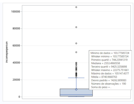
The dataset provided for this assignment has 16 variables and 213 observations. From the variables, I choose to analyze income per person (incomeperperson) and life expectancy (lifeexpectancy). The moderator is urban rate (urbanrate). The income per person is measured by the Gross Domestic Product per capita in constant 2.000 US$ (2010). And the life expectancy at birth (years) is the average number of years a newborn child would live if current mortality patterns were to stay the same. And the urban rate is % of total population that lives in urban areas (2008).

The Question

Are income per person and life expectancy associated for low urban rate countries? And income per person and life expectancy associated for high urban rate countries? In other words, our explanatory variable associated with our response variable, for each population sub-group? We are using a third variable to understand if this variable effects the direction and or strength of the relation between our explanatory and response variable.

To understand the two variables, I analyze the boxplots posted below.

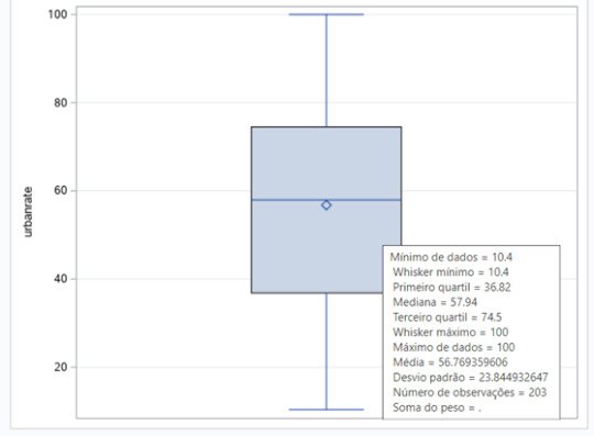
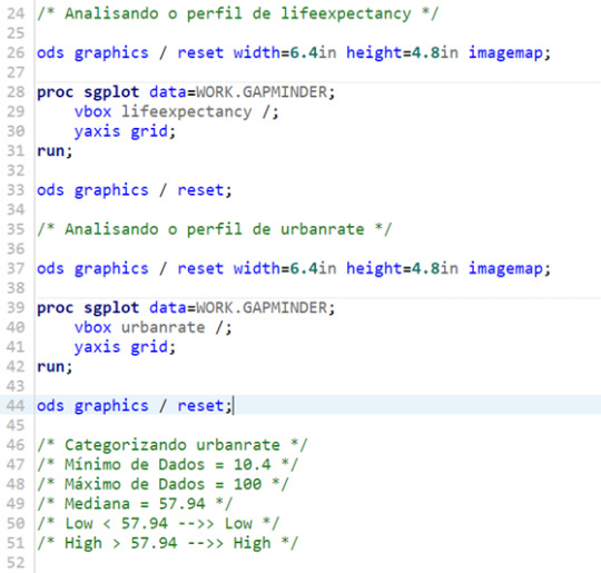
Since urban rate is a quantitative variable, I had to transform it into a categorical variable. I created a sub-group for low urban rate countries and another one to a high urban rate countries.

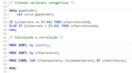
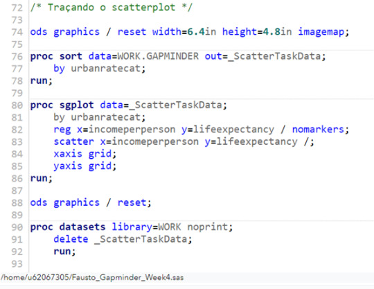
The SAS Studio Code

For this assignment, I decided to code on SAS Studio, since the tool was new for me, and it was an opportunity to gain experience. The code is posted below. The comments are in Portuguese, my mother tongue.

Results – Pearson Correlation Coefficient (r) for both groups

Aiming to answer the question of the assignment, I ran a correlation procedure to obtain the Pearson Correlation Coefficient (r) for both groups. The results of the test showed a P value 0.0001. So, the test is valid, and we can analyze the results of the two sub-groups.

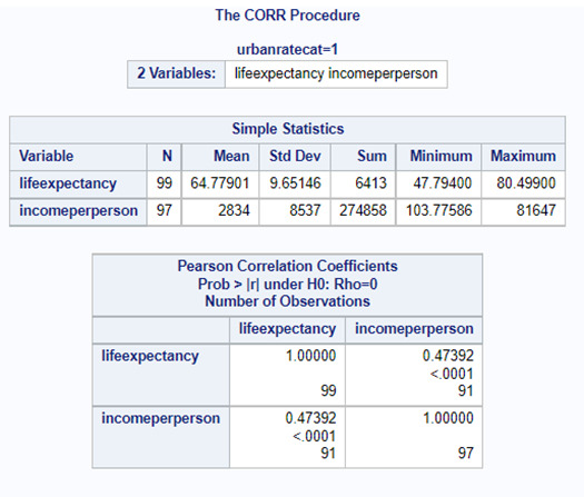
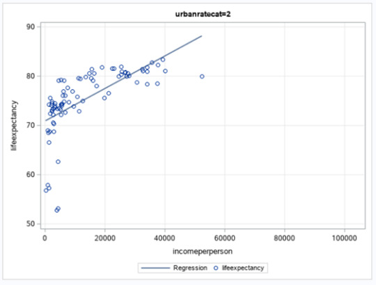
Since the r obtained is positive, we have a positive correlation between income per person and life expectancy for both groups. The correlation is stronger for the second group, the countries with higher urban rate. The r in this group is 0.63784. For the first group, the r obtained is 0.47392. These conclusions can also be seen in two the scatter plot posted below. We can see too much dispersion, when we display the points of the countries at the graph.

The r2 for the first sub-group (low urban rate) is 0.2246. The r2 is the fraction of the variability of one variable that can be predicted by the other. So, if we know the income per person, we can predict only 22.46% of the variability we will see in the rate of life expectancy.

For the second sub-group (high urban rate), the r2 is 0,4068. If we know the income per person, we can predict only 40.68% of the variability we will see in the rate of life expectancy, almost the double of the first sub-group.

[faustokeske]

Generating a Correlation Coefficient

by Fausto Keske

Introduction

This is the third assignment (Week 3) of the course Data Analysis Tools from the Wesleyan University at the Coursera Platform. Now, the challenge is to generate a Correlation Coefficient. This type of coefficient is used when you have two quantitative variables. For this assignment, as asked, I will use the Pearson Correlation Coefficient (r) that is a numerical measure of a linear relationship between two quantitative variables.

Case Study – Gap Minder

Gap Minder was founded in Stockholm by Ola, Anna and Hans Rosling. The company is a non-profit venture promoting sustainable global development and the achievement of the United Nations Millenium Development Goals. It seeks to increase the use and understanding of statistics about social, economic, and environmental development at local, national and global levels. Its website is mind blowing, everybody should visit it: https://www.gapminder.org/.

The dataset provided for this assignment has 16 variables and 213 observations. From the variables, I choose to analyze alcconsumption and lifeexpectancy. The alcohol consumption per adult (age 15+) is measured by how many liters recorded and estimated average alcohol consumption. And the life expectancy at birth (years) is the average number of years a newborn child would live if current mortality patterns were to stay the same.

The Question

Is there a correlation between alcohol consumption and life expectancy?

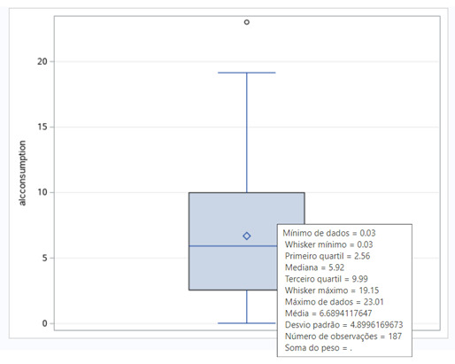
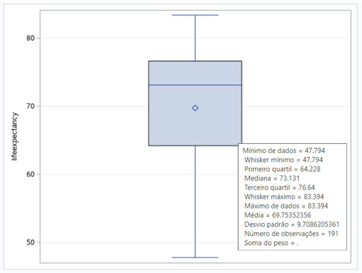
To understand the two variables, I analyze the boxplots posted below.

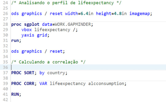
The SAS Studio Code

For this assignment, I decided to code on SAS Studio, since the tool was new for me, and it was an opportunity to gain experience. The code is posted below. The comments are in Portuguese, my mother tongue.

Results – Pearson Correlation Coefficient (r)

Aiming to answer the question of the assignment, I ran a correlation procedure to obtain the Pearson Correlation Coefficient (r). The results of the test showed a P value 0.0001. So, the test is valid, and we can analyze the results.

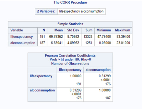
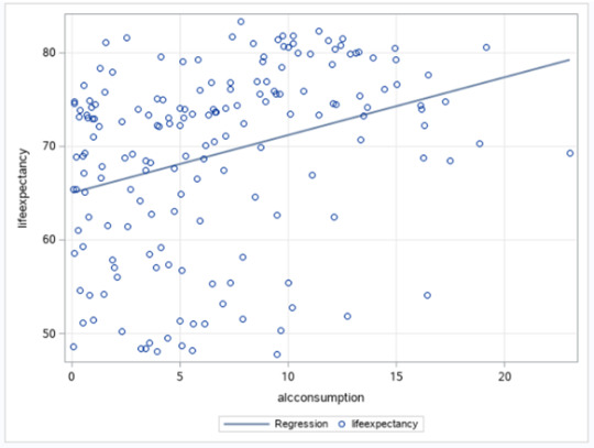
Since the r obtained is positive, we have a positive correlation between alcohol consumption and life expectancy. But this correlation is not strong, since our r is 0.31299, and the possible range is from -1 to +1. This conclusion can also be seen in the scatter plot posted below. We can see too much dispersion, when we display the points of the countries at the graph.

The r2 of this test is 0.098. The r2 is the fraction of the variability of one variable that can be predicted by the other. So, if we know the alcohol consumption, we can predict only 9.8% of the variability we will see in the rate of life expectancy.

[faustokeske]

Running a Chi-Square Test of Independence

by Fausto Keske

Introduction

This is the second assignment (Week 2) of the course Data Analysis Tools from the Wesleyan University at the Coursera Platform. Now, the challenge is to run a Chi-Square Test of Independence. This type of analysis is used when you have two categorical variables. The null hypothesis is that there is no relationship between the two categorical variables, we can say that they are independent, while the alternative hypothesis is that there is a relationship between the two categorical variables, we can say that they are not independent. If your research question does not include a categorical variable, you can categorize one that is quantitative, which was the case of this assignment.

Case Study – Gap Minder

Gap Minder was founded in Stockholm by Ola, Anna and Hans Rosling. The company is a non-profit venture promoting sustainable global development and the achievement of the United Nations Millenium Development Goals. It seeks to increase the use and understanding of statistics about social, economic and environmental development at local, national and global levels. Its website is mind blowing, everybody should visit it: https://www.gapminder.org/.

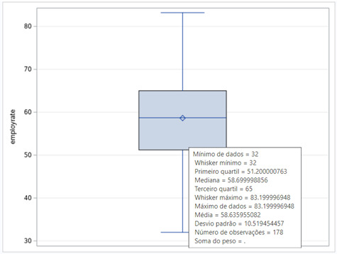
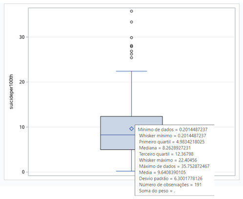
The dataset provided for this assignment has 16 variables and 213 observations. From the variables, I choose to analyze employ rate (employrate), and suicide per 100.000 (suicideper100TH). The employ rate is a percentage of total population, age above 15, that has been employed during the given year. And the suicide per 100.000 is the mortality due to self-inflicted injury, per 100.000 standard population, age adjusted.

The Question

Is the employ rate and suicide per 100TH dependence independent or dependent?

Ho | There is no difference. Employ rate and suicide 100TH are independent.

Ha | There is a difference. Employ rate and suicide 100TH are not independent.

Since both variables are quantitative, I had to transform them into categorical variables. For the parameters, I analyze the boxplots posted below.

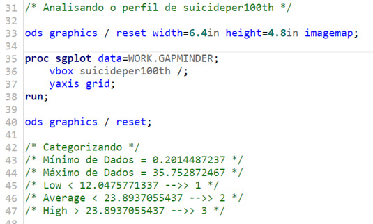
The SAS Studio Code

For this assignment, I decided to code on SAS Studio, since the tool was new for me, and it was an opportunity to learn it. The code is posted below. The comments are in Portuguese, my mother tongue.

Results – Statistical Test ANOVA

Aiming to answer the question of the assignment, I ran a statistical test Chi-Square. The results of the test showed a P value 0.0669. So, we reject the alternative hypothesis (Ha) and assume the Ho as true. So, we can get to the conclusion that there is no relationship between employ rate and suicide 100TH, they are independent.

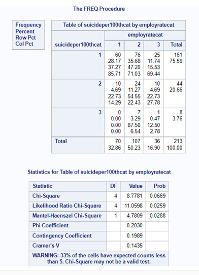
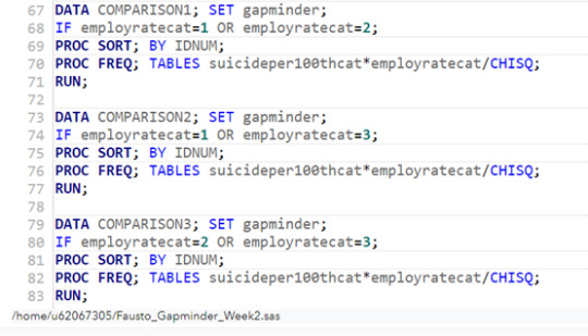
If the P value were smaller than 0.05, we could accept the alternative hypothesis and say that employ rate and suicide 100TH are not independent. In that case, we should run a post hoc test for Chi Square tests of independence. Is this test we need to perform comparisons for each pair of employ rate across the three suicide per 100TH category. As part of the learning process, I ran the comparisons, and they are posted below.

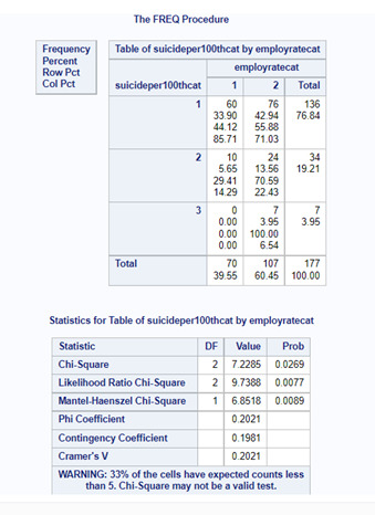
Comparison1 (employ rate category 1 vs. employ rate category 2)

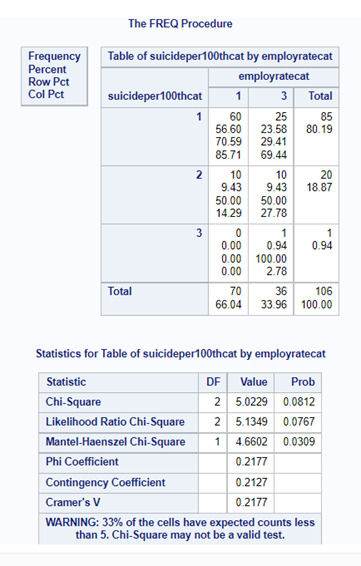
Comparison2 (employ rate category 1 vs. employ rate category 3)

Comparison3 (employ rate category 2 vs. employ rate category 3)

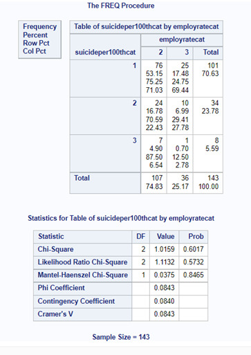
For these comparisons, we should use an adjusted Bonferroni P value. Since we had 3 comparisons, the adjusted P value should be 0.017 (0.05/3). This way we can protect our test against type 1 error. I will not analyze the results of the comparisons, because they are not valid, since our P value for the Chi Square test is higher than 0.05.

[faustokeske]

Running an Analysis of Variance

by Fausto Keske

Introduction

This is the first assignment (Week 1) of the course Data Analysis Tools from the Wesleyan University at the Coursera Plataform. The challenge is to run an Analysis of Variance using the Statistical Test ANOVA. This type of analysis assesses whether the means of two or more groups are statistically different from each other. It is used whenever you want to compare the means (quantitative variables) of groups (categorical variables). The null hypothesis is that there is no difference in the mean of the quantitative variable across groups (categorical variable), while the alternative is that there is a difference. If your research question does not include a categorical variable, you can categorize one that is quantitative, which was the case of this assignment.

Case Study – Gap Minder

Gap Minder was founded in Stockholm by Ola, Anna and Hans Rosling. The company is a non-profit venture promoting sustainable global development and the achievement of the United Nations Millenium Development Goals. It seeks to increase the use and understanding of statistics about social, economic and environmental development at local, national and global levels. Its website is mind blowing, everybody should visit it: https://www.gapminder.org/.

The dataset provided for this assignment has 16 variables and 213 observations. From the variables, I choose to analyze income per person (incomeperperson) and life expectancy (lifeexpectancy).

The Question

Is the life expectancy different among four categories of income per person (low income, average low income, average high income and high income)?

Ho | There is no difference. Life expectancy and income per person are not related.

Ha | There is a difference. Life expectancy and income per person are related.

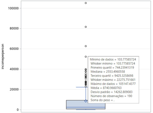
Since the income per person is a quantitative variable, I had to transform it into a categorical variable. For the parameters, I analyzed the boxplot posted below.

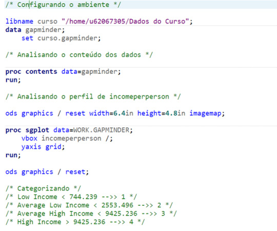
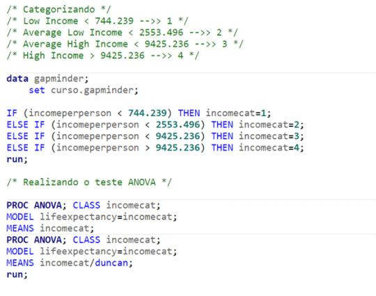
The SAS Studio Code

For this assignment, I decided to code on SAS Studio, since the tool was new for me, and it was an opportunity to learn it. The code is posted below. The comments are in Portuguese, my mother tongue.

Results – Statistical Test ANOVA

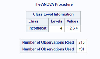
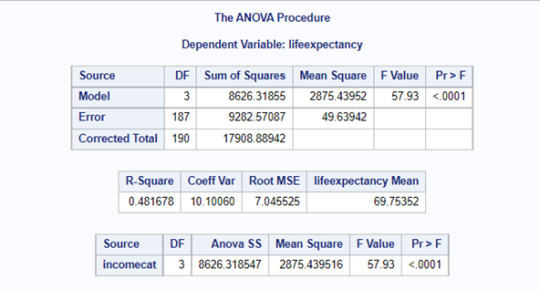
Aiming to answer the question of the assignment, I ran a statistical test ANOVA. As shown below, from the 213 observations, 191 were used for the test.

The results of test showed that the F value is 57.93 and the P value 0.0001. So, we can accept the alternative hypothesis (Ha) and get to the conclusion that life expectancy and income per person are related. There are differences in the means of life expectancy among the four categories of income per person.

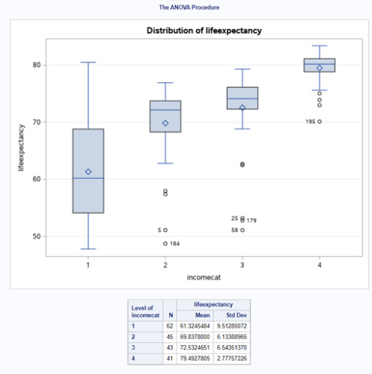
The ANOVA test also deliveries a boxplot for each category (below) and, as we can see, the life expectancy of the mean of the first category (low income) is 61.32 years. The 2 (average low) and 3 (average high) categories have 69.83 and 72.53 years of life expectancy. And the high category (4) has a mean of 79.49 years of life expectancy.

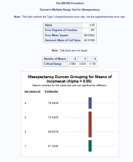
So far so good, we can determine that there are differences among the groups, but we can not tell which groups are different from the others. To obtain this answer, I applied the Duncan test, a post hoc test. The test showed (below) that the categories 2 and 3 are not significantly different, because they appeared at the same bar group. But we can see significant differences from the others in groups 1 (low income) and group 4 (high income).