#statistical test

[eduardotleite]

ANOVA Analysis

This is the task of Week 1 of the course Data Analysis Tools at the Coursera Plataform. The challenge is to execute an Analysis of Variance using the ANOVA Statistical Test. This type of analysis assesses whether the means of two or more groups are statistically different from each other. Is used whenever you want to compare the means (quantitative variables) of groups (categorical variables). The null hypothesis is that there is no difference in the mean of the quantitative variable across groups (categorical variable), while the alternative is that there is a difference.

DataSet Used – Gap Minder Gapminder identifies systematic misconceptions about important global trends and proportions and uses reliable data to develop easy to understand teaching materials to rid people of their misconceptions. Gapminder is an independent Swedish foundation with no political, religious, or economic affiliations. should visit it: https://www.gapminder.org/.

The dataset used has 16 variables and 213 rows. I choosed to analyze income per person (incomeperperson) and life expectancy (lifeexpectancy).

And how is the Question?

Is the life expectancy different among four categories of income per person (A,B,C,D,E)?

Since the income per person is a quantitative variable, I transformed it into a categorical variable, using parameters sugested by IBGE to classify the social class of according of income. For the parameters, I analyzed the boxplot posted below.

the data in image is in portuguese, because the IBGE is an Brazilian institute.

The Code

I used the Anaconda to code in Python for this task. The code is posted below.

import numpy import pandas as pd import statsmodels.api as sm import statsmodels.formula.api as smf import statsmodels.stats.multicomp as multi import matplotlib.pyplot as plt import seaborn as sns import researchpy as rp import pycountry_convert as pc

df = pd.read_csv('gapminder.csv') df = df[['lifeexpectancy', 'incomeperperson']]

df['lifeexpectancy'] = df['lifeexpectancy'].apply(pd.to_numeric, errors='coerce') df['incomeperperson'] = df['incomeperperson'].apply(pd.to_numeric, errors='coerce')

def income_categories(row): if row["incomeperperson"]>15000: return "A" elif row["incomeperperson"]>5000: return "B" elif row["incomeperperson"]>3000: return "C" elif row["incomeperperson"]>1000: return "D" else: return "E"

df=df[(df['lifeexpectancy']>=1) & (df['lifeexpectancy']<=120) & (df['incomeperperson'] > 0) ]

df["Income_category"]=df.apply(income_categories, axis=1)

df = df[["Income_category","incomeperperson","lifeexpectancy"]].dropna()

df["Income_category"]=df.apply(income_categories, axis=1)

print (rp.summary_cont(df['lifeexpectancy']))

fig1, ax1 = plt.subplots() df_new = [df[df['Income_category']=='A']['lifeexpectancy'], df[df['Income_category']=='B']['lifeexpectancy'], df[df['Income_category']=='C']['lifeexpectancy'], df[df['Income_category']=='D']['lifeexpectancy'], df[df['Income_category']=='E']['lifeexpectancy']] ax1.set_title('life expectancy') ax1.boxplot(df_new) plt.show()

results = smf.ols('lifeexpectancy ~ C(Income_category)', data=df).fit() print (results.summary())

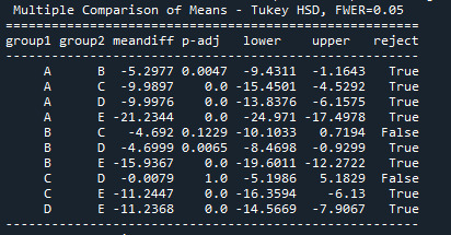
print ("Tukey") mc1 = multi.MultiComparison(df['lifeexpectancy'], df['Income_category']) print (mc1) res1 = mc1.tukeyhsd() print (res1.summary())

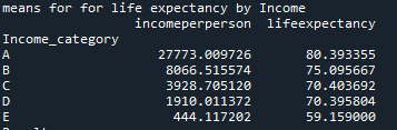
print ('means for for life expectancy by Income') m1= df.groupby('Income_category').mean() print (m1)

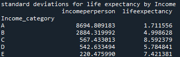
print ('Results') print ('standard deviations for life expectancy by Income') sd1 = df.groupby('Income_category').std() print (sd1)

Results – ANOVA Analysis

Aiming to answer the question of the task, I ran a test ANOVA. As shown below, from the 176 rows, 171 were used for the test, i have used a filter to remove some wrong values, as non numeric, negative, etc, reducing the rows of the original dataset

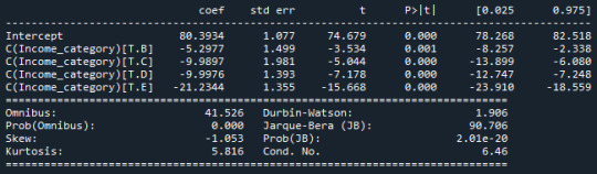
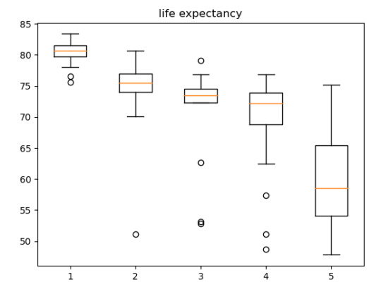
The ANOVA analysis shows a graph for each category (above) and, as we can see, the life expectancy of A class, have the life expectative of 80.39 years while the E class have the life expectative of 59.15 years.

[dejwrldarchived]

the topic of colorism within the black community will never be understood until people understand that it's deeper than being bullied in high school and dating preferences.

[jadagul]

I am spectacularly offended by this Matt Levine reader email about using astrology in consumer finance prediction.

This was a machine learning model – the job of the data scientist was, put everything in, see what's significant, of that discard everything that's discriminatory, the rest is your model. Ultimately with twelve astrological signs it's over 50/50 that one will come out significant at 95%. I thought it was elegant. "Astrological signs? Do you believe that?" my boss said. I said it wasn't a question of belief, I was a statistician and was going to follow the numbers rather than letting anyone's preexisting theories about the stars and planets influence the data science. I think he believed that meant I'd agreed to take it out.

Like, the guy literally said "We're very likely to have a false positive here by chance, but since we got one we have to take it seriously. I'm a statistician."

He's fully aware that he's p-hacking and garden-pathing. He's fully aware of the multiple comparisons problem. And then he endorses the conclusion anyway!

(And, as a side note, it's not over 50/50; If you do twelve tests the chance of one coming out significant by chance is about 46%. So he fucked up the arithmetic too!)

[birat-69]

can’t be asked to colour rn so here’s a timelapse of my favourite drawing of my favourite hermits :))

[jackslesbiansubconcious]

Me rn:

[heyhelloitsmilo]

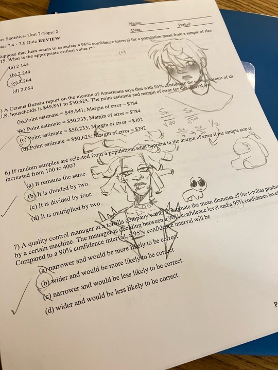
statistics is so easy

[hazellvsq]

hazel & thanatos : nico & cupid scene comparison

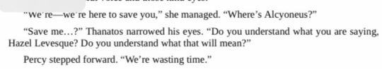
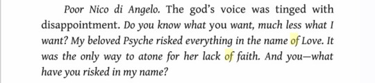
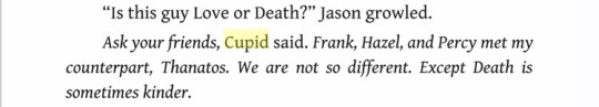
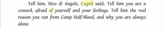
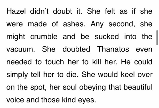
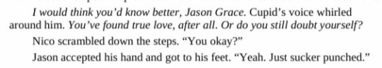
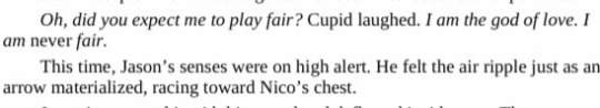
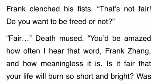
both of these scenes are about identity and truth at odds with innate self-preservation. both gods reference each other and acknowledge their similarities. cupid references hazel, and thanatos even references nico (didn't include that scene but hazel asks thanatos if he knows where nico is). jason and frank both also face obstacles through these gods, but the true tests are for nico and hazel. the point of both scenes is to demand that both characters face their greatest fears, and force hazel and nico to be honest about why they have come so far on their respective journeys, and admit what is is that they truly want. also, thanatos is fairly passive and hazel experiences more visceral attraction to him than she does to her series love interests, whereas nico's confession is very blunt and unromantic, and cupid is very violent, causing physical and emotional agony and further blurring the domains of the two gods.

[carbonateds-oda]

skk stans have some NERVE complaining abt that one panel not getting animated like have y’all seen what they did to the entire first light novel?? kndz stans have been in the trenches from the very start I DONT WANNA HEAR IT

[whirling-ghost]

I'm actually impressed that I made it to 2024 before getting a positive covid test

i will need to dig out that "queer people should know better than to assign morality to a virus" post because I'm gonna need it when the anxiety kicks it

[itsalwaysjune]

17.05.24

The weather is nice again! I'm glad the rain definitely dampened my mood.

I spent almost the entire day in the library- found 'You will beat this essay' written on the cublicle wall, it gave me the motivation I needed to get a big chunk of my Lab reoprt done.

Today I;

Did the introduction of my lab report

Did the methodology of my lab report

Created the Figures for my lab report

Started to contact the study abroad students I will be travelling with

Studied social categorisation, stereotyping and prejudice

Studied intergroup relations and conflict

I went to the library and forgot my tablet, so I had to walk all the way there and alllll the way back.

[glitter-alienz]

She standard on my deviation til I mean

[woolieshubris]

huge dub for nonbinary people in oregon

[newtness532]

remember when i said i have a lot of things i need to do today and then i did none of that?

[virmire]

someone explain two way ANOVA test to me like I’m a toddler lol

[ukuraichu]

losing my mind. can i bust this ghost. who knows

[vraska-theunseen]

i keep dismissing societal concepts i think are silly in my head and so i go around being like we made this up it's so pointless... abt like copyright law or whatever but then i kind of lock myself in an echo chamber of my own brain where i go around thinking stuff and then i have a conversation with a friend where i find out they put weight in [concept] i've dismissed like they're talking about how IQ is real and measurable and important for statistics and im like WHAT THE HELL...