#pearson correlation coefficient

[regressingnow]

Per-Capita Income and Life Expectancy : W3 Data Analysis Tools

For the third week’s assignment of Data Analysis Tool on Coursera, we would continue to be working with GapMinder's dataset which contains statistics in the social, economic, and environmental development variable at local, national, and global levels

We would be studying the effect of Income per Person of a County on prevalent rates of life-expectancy. Since both the explanatory variable (Per-Capita Income) and the response variable are quantitative we'll calculate the Pearson Correlation Coefficient to analyze the strength of correlation between the variables.

The Correlation Analysis between the two variables gives :

The Correlation Coefficient is 0.60 with a very low p-value << 0.0001, which indicates a considerably strong and significant relation between the Per-Capita Income and the Life Expectancy of individuals. A positive Correlation Coefficient indicates that the Life-Expectancy increases with the Per-Capita Income of a Country.

However, looking at the scatter-plot between the two variables, we see that a sharp increase in the life expectancy is seen only at the very low end of the per-capita income spectrum. Beyond a per-capita income of 10000, the life-expectancy almost flattens out. So, we need to understand the strong relationship between the variables together the scatter-plot.

[nickfoxer]

Why a Spinoff for Tarlos Is Feasible,Based on AO3 Data.

In this article,I will explain why the decline in Tarlos'popularity is an illusion and why Tarlos'popularity is rebounding and has a solid and reliable core audience in the long term.

It is well-known in American TV shows that the popularity of a ship is reflected in the annual increase of AO3 tags.The popularity of a ship is associated with many factors,such as the director's skills,the scriptwriter's plot design,and the chemistry between actors.

When the director,scriptwriter,and production team remain the same across seasons of the same TV show,these factors may fluctuate but the changes are relatively small.In such cases,people often overlook a key factor affecting the annual increase of AO3 tags:the number of episodes aired in a season!

(Top 100 in 2021,2022 and 2023)

For example,in 2023,compared to 2024,the annual increase of AO3 tags for"TK/Carlos"declined and exited the top 100 for the first time since 2021.Does this mean Tarlos is no longer popular?On the contrary,the conclusion is incorrect because it ignores the number of episodes aired each season.

9-1-1:Lone Star from 2020 to 2023,each year saw a complete season aired,while only nine episodes were broadcast in Season 5 in 2024.

According to the Pearson correlation coefficient formula,the annual increase of tags is strongly positively correlated with the total number of episodes per year(referred to as"episodes").

The correlation coefficient : r≈ 0.645

In statistics,when 0.7≤|r|≤ 1,two factors are considered to have a strong correlation.However,from Seasons 1 to 4,there were fluctuations in production quality.Season 4 had the lowest ratings on various review websites compared to the previous three seasons.Did this fundamental factor affect the tag increase in 2023?

To test this hypothesis,we removed the data from Season 4 and recalculated the Pearson correlation coefficient using data from Seasons 1,2,3,and 5.

The new correlation coefficient：r'≈ 0.845

We then conducted a hypothesis test to verify the p-value:(0.05<p<0.1),which means the correctness rate of the correlation is over 90%.

Thus,under similar production standards,the number of episodes in9-1-1:Lone Starand the annual increase of"Carlos/TK"AO3 tags have a very strong positive correlation.

We can conclude that the main reason for the drop of"TK/Carlos"out of the top 100 in 2024 was the reduced number of episodes aired that year.

Apart from statistical analysis,other factors also played a role:

1. Season 5 premiered at the end of September.By the cutoff date for the rankings(January 1,2025),only nine episodes had been aired.Many viewers hadn't had time to watch,and many fan fiction authors hadn't had time to write.

2. Previous seasons(Seasons 1-4)were broadcast at the beginning or middle of the year,finishing by September at the latest.They attracted viewers for most of the year.In contrast,Season 5 only had three months(from September to December)to attract viewers.

3. The gap between the premiere of Season 5 and the last episode of the previous season was as long as 13 months,longer than the gap between any other seasons.

4. Season 5 had the least official promotion,relying almost entirely on the actors'personal promotions.

In fact,Tarlos'popularity has not declined but increased.The reduced number of episodes in 2024 affected the data and led to a misjudgment.

Focusing on the last column:The Average Contribution per Episode to the Annual Increase in Tags.

In 2024,each of the nine episodes contributed an average of about 150 tags.Compared to last year's figure of 85.8,this represents a year-on-year growth rate of 74.83%.Looking at the past five years,the average contribution per episode this year is close to the historical high,almost comparable to the peak in 2021.

From this analysis,we can see that Tarlos'popularity has been steadily rising since the debut of9-1-1:Lone Starin 2020,reaching its peak in 2021,then entering a stable period,and finally hitting another peak in 2024.

Tarlos has the potential for sustainable growth.If a Spinoff featuring them were to air on streaming platforms or other good platforms,their stable audience and fan base would continue to contribute to the popularity and discussion of Tarlos.

Conclusion:Tarlos has a solid and reliable core audience with the potential for sustainable development and long-term success.

Given the relatively low cost and high return on investment for a derivative series,it is highly feasible.As long as the scriptwriting quality of the derivative series can maintain the level of the original,continued success is not only possible but likely—even more so than before.🔥

[ozzgin]

How you come with that fuckin lore sheet (like not even in my messiest dreams I could connect all of your writings 😭😭)

There is a small chance that my need to organize literal figments of imagination might be related to my ‘tism. Can’t say for sure, I’ll have to run a correlation test in SPSS and get back to you once I have a Pearson coefficient.

I’m also uncertain whether you’re referring to the reader guide featuring my old stories, or the recent human kink compilation (I’m guessing the latter), but it sadly doesn’t change the verdict.

[myrawjcsmicasereports]

 Inhibition of EIF4E Downregulates VEGFA and CCND1 Expression to Suppress Ovarian Cancer Tumor Progression by Jing Wang in Journal of Clinical Case Reports Medical Images and Health Sciences

Abstract

This study investigates the role of EIF4E in ovarian cancer and its influence on the expression of VEGFA and CCND1. Differential expression analysis of VEGFA, CCND1, and EIF4E was conducted using SKOV3 cells in ovarian cancer patients and controls. Correlations between EIF4E and VEGFA/CCND1 were assessed, and three-dimensional cell culture experiments were performed. Comparisons of EIF4E, VEGFA, and CCND1 mRNA and protein expression between the EIF4E inhibitor 4EGI-1-treated group and controls were carried out through RT-PCR and Western blot. Our findings demonstrate elevated expression of EIF4E, VEGFA, and CCND1 in ovarian cancer patients, with positive correlations. The inhibition of EIF4E by 4EGI-1 led to decreased SKOV3 cell clustering and reduced mRNA and protein levels of VEGFA and CCND1. These results suggest that EIF4E plays a crucial role in ovarian cancer and its inhibition may modulate VEGFA and CCND1 expression, underscoring EIF4E as a potential therapeutic target for ovarian cancer treatment.

Keywords: Ovarian cancer; Eukaryotic translation initiation factor 4E; Vascular endothelial growth factor A; Cyclin D1

Introduction

Ovarian cancer ranks high among gynecological malignancies in terms of mortality, necessitating innovative therapeutic strategies [1]. Vascular endothelial growth factor (VEGF) plays a pivotal role in angiogenesis, influencing endothelial cell proliferation, migration, vascular permeability, and apoptosis regulation [2, 3]. While anti-VEGF therapies are prominent in malignancy treatment [4], the significance of cyclin D1 (CCND1) amplification in cancers, including ovarian, cannot be overlooked, as it disrupts the cell cycle, fostering tumorigenesis [5, 6]. Eukaryotic translation initiation factor 4E (EIF4E), central to translation initiation, correlates with poor prognoses in various cancers due to its dysregulated expression and activation, particularly in driving translation of growth-promoting genes like VEGF [7, 8]. Remarkably, elevated EIF4E protein levels have been observed in ovarian cancer tissue, suggesting a potential role in enhancing CCND1 translation, thereby facilitating cell cycle progression and proliferation [9]. Hence, a novel conjecture emerges: by modulating EIF4E expression, a dual impact on VEGF and CCND1 expression might be achieved. This approach introduces an innovative perspective to impede the onset and progression of ovarian cancer, distinct from existing literature, and potentially offering a unique therapeutic avenue.

Materials and Methods

Cell Culture

Human ovarian serous carcinoma cell line SKOV3 (obtained from the Cell Resource Center, Shanghai Institutes for Biological Sciences, Chinese Academy of Sciences) was cultured in DMEM medium containing 10% fetal bovine serum. Cells were maintained at 37°C with 5% CO2 in a cell culture incubator and subcultured every 2-3 days.

Three-Dimensional Spheroid Culture

SKOV3 cells were prepared as single-cell suspensions and adjusted to a concentration of 5×10^5 cells/mL. A volume of 0.5 mL of single-cell suspension was added to Corning Ultra-Low Attachment 24-well microplates and cultured at 37°C with 5% CO2 for 24 hours. Subsequently, 0.5 mL of culture medium or 0.5 mL of EIF4E inhibitor 4EGI-1 (Selleck, 40 μM) was added. After 48 hours, images were captured randomly from five different fields—upper, lower, left, right, and center—using an inverted phase-contrast microscope. The experiment was repeated three times.

GEPIA Online Analysis

The GEPIA online analysis tool (http://gepia.cancer-pku.cn/index.html) was utilized to assess the expression of VEGFA, CCND1, and EIF4E in ovarian cancer tumor samples from TCGA and normal samples from GTEx. Additionally, Pearson correlation coefficient analysis was employed to determine the correlation between VEGF and CCND1 with EIF4E.

RT-PCR

RT-PCR was employed to assess the mRNA expression levels of EIF4E, VEGF, and CCND1 in treatment and control group samples. Total RNA was extracted using the RNA extraction kit from Vazyme, followed by reverse transcription to obtain cDNA using their reverse transcription kit. Amplification was carried out using SYBR qPCR Master Mix as per the recommended conditions from Vazyme. GAPDH was used as an internal reference, and the primer sequences for PCR are shown in Table 1.

Amplification was carried out under the following conditions: an initial denaturation step at 95°C for 60 seconds, followed by cycling conditions of denaturation at 95°C for 10 seconds, annealing at 60°C for 30 seconds, repeated for a total of 40 cycles. Melting curves were determined under the corresponding conditions. Each sample was subjected to triplicate experiments. The reference gene GAPDH was used for normalization. The relative expression levels of the target genes were calculated using the 2-ΔΔCt method.

Western Blot

Western Blot technique was employed to assess the protein expression levels of EIF4E, VEGF, and CCND1 in the treatment and control groups. Initially, cell samples collected using RIPA lysis buffer were lysed, and the total protein concentration was determined using the BCA assay kit (Shanghai Biyuntian Biotechnology, Product No.: P0012S). Based on the detected concentration, 20 μg of total protein was loaded per well. Electrophoresis was carried out using 5% stacking gel and 10% separating gel. Subsequently, the following primary antibodies were used for immune reactions: rabbit anti-human polyclonal antibody against phospho-EIF4E (Beijing Boao Sen Biotechnology, Product No.: bs-2446R, dilution 1:1000), mouse anti-human monoclonal antibody against EIF4E (Wuhan Sanying Biotechnology, Product No.: 66655-1-Ig, dilution 1:5000), mouse anti-human monoclonal antibody against VEGFA (Wuhan Sanying Biotechnology, Product No.: 66828-1-Ig, dilution 1:1000), mouse anti-human monoclonal antibody against CCND1 (Wuhan Sanying Biotechnology, Product No.: 60186-1-Ig, dilution 1:5000), and mouse anti-human monoclonal antibody against GAPDH (Shanghai Biyuntian Biotechnology, Product No.: AF0006, dilution 1:1000). Subsequently, secondary antibodies conjugated with horseradish peroxidase (Shanghai Biyuntian Biotechnology, Product No.: A0216, dilution 1:1000) were used for immune reactions. Finally, super-sensitive ECL chemiluminescence reagent (Shanghai Biyuntian Biotechnology, Product No.: P0018S) was employed for visualization, and the ChemiDocTM Imaging System (Bio-Rad Laboratories, USA) was used for image analysis.

Statistical Analysis

GraphPad software was used for statistical analysis. Data were presented as (x ± s) and analyzed using the t-test for quantitative data. Pearson correlation analysis was performed for assessing correlations. A significance level of P < 0.05 was considered statistically significant.

Results

3D Cell Culture of SKOV3 Cells and Inhibitory Effect of 4EGI-1 on Aggregation

In this experiment, SKOV3 cells were subjected to 3D cell culture, and the impact of the EIF4E inhibitor 4EGI-1 on ovarian cancer cell aggregation was investigated. As depicted in Figure 1, compared to the control group (Figure 1A), the diameter of the SKOV3 cell spheres significantly decreased in the treatment group (Figure 1B) when exposed to 4EGI-1 under identical culture conditions. This observation indicates that inhibiting EIF4E expression effectively suppresses tumor aggregation.

Expression and Correlation Analysis of VEGFA, CCND1, and EIF4E in Ovarian Cancer Samples

To investigate the expression of VEGFA, CCND1, and EIF4E in ovarian cancer, we utilized the GEPIA online analysis tool and employed the Pearson correlation analysis method to compare expression differences between tumor and normal groups. As depicted in Figures 2A-C, the results indicate significantly elevated expression levels of VEGFA, CCND1, and EIF4E in the tumor group compared to the normal control group. Notably, the expression differences of VEGFA and CCND1 were statistically significant (p < 0.05). Furthermore, the correlation analysis revealed a positive correlation between VEGFA and CCND1 with EIF4E (Figures 2D-E), and this correlation exhibited significant statistical differences (p < 0.001). These findings suggest a potential pivotal role of VEGFA, CCND1, and EIF4E in the initiation and progression of ovarian cancer, indicating the presence of intricate interrelationships among them.

EIF4E, VEGFA, and CCND1 mRNA Expression in SKOV3 Cells

To investigate the function of EIF4E in SKOV3 cells, we conducted RT-PCR experiments comparing EIF4E inhibition group with the control group. As illustrated in Figure 3, treatment with 4EGI-1 significantly reduced EIF4E expression (0.58±0.09 vs. control, p < 0.01). Concurrently, mRNA expression of VEGFA (0.76±0.15 vs. control, p < 0.05) and CCND1 (0.81±0.11 vs. control, p < 0.05) also displayed a substantial decrease. These findings underscore the significant impact of EIF4E inhibition on the expression of VEGFA and CCND1, indicating statistically significant differences.

Protein Expression Profiles in SKOV3 Cells with EIF4E Inhibition and Control Group

Protein expression of EIF4E, VEGFA, and CCND1 was assessed using Western Blot in the 4EGI-1 treatment group and the control group. As presented in Figure 4, the expression of p-EIF4E was significantly lower in the 4EGI-1 treatment group compared to the control group (0.33±0.14 vs. control, p < 0.001). Simultaneously, the expression of VEGFA (0.53±0.18 vs. control, p < 0.01) and CCND1 (0.44±0.16 vs. control, p < 0.001) in the 4EGI-1 treatment group exhibited a marked reduction compared to the control group.

Discussion

EIF4E is a post-transcriptional modification factor that plays a pivotal role in protein synthesis. Recent studies have underscored its critical involvement in various cancers [10]. In the context of ovarian cancer research, elevated EIF4E expression has been observed in late-stage ovarian cancer tissues, with low EIF4E expression correlating to higher survival rates [9]. Suppression of EIF4E expression or function has been shown to inhibit ovarian cancer cell proliferation, invasion, and promote apoptosis. Various compounds and drugs that inhibit EIF4E have been identified, rendering them potential candidates for ovarian cancer treatment [11]. Based on the progressing understanding of EIF4E's role in ovarian cancer, inhibiting EIF4E has emerged as a novel therapeutic avenue for the disease. 4EGI-1, a cap-dependent translation small molecule inhibitor, has been suggested to disrupt the formation of the eIF4E complex [12]. In this study, our analysis of public databases revealed elevated EIF4E expression in ovarian cancer patients compared to normal controls. Furthermore, through treatment with 4EGI-1 in the SKOV3 ovarian cancer cell line, we observed a capacity for 4EGI-1 to inhibit SKOV3 cell spheroid formation. Concurrently, results from PCR and Western Blot analyses demonstrated effective EIF4E inhibition by 4EGI-1. Collectively, 4EGI-1 effectively suppresses EIF4E expression and may exert its effects on ovarian cancer therapy by modulating EIF4E.

Vascular Endothelial Growth Factor (VEGF) is a protein that stimulates angiogenesis and increases vascular permeability, playing a crucial role in tumor growth and metastasis [13]. In ovarian cancer, excessive release of VEGF by tumor cells leads to increased angiogenesis, forming a new vascular network to provide nutrients and oxygen to tumor cells. The formation of new blood vessels enables tumor growth, proliferation, and facilitates tumor cell dissemination into the bloodstream, contributing to distant metastasis [14]. As a significant member of the VEGF family, VEGFA has been extensively studied, and it has been reported that VEGFA expression is notably higher in ovarian cancer tumors [15], consistent with our public database analysis. Furthermore, elevated EIF4E levels have been associated with increased malignant tumor VEGF mRNA translation [16]. Through the use of the EIF4E inhibitor 4EGI-1 in ovarian cancer cell lines, we observed a downregulation in both mRNA and protein expression levels of VEGFA. This suggests that EIF4E inhibition might affect ovarian cancer cell angiogenesis capability through downregulation of VEGF expression.

Cyclin D1 (CCND1) is a cell cycle regulatory protein that participates in controlling cell entry into the S phase and the cell division process. In ovarian cancer, overexpression of CCND1 is associated with increased tumor proliferation activity and poor prognosis [17]. Elevated CCND1 levels promote cell cycle progression, leading to uncontrolled cell proliferation [18]. Additionally, CCND1 can activate cell cycle-related signaling pathways, promoting cancer cell growth and invasion capabilities [19]. Studies have shown that CCND1 gene expression is significantly higher in ovarian cancer tissues compared to normal ovarian tissues [20], potentially promoting proliferation and cell cycle progression through enhanced cyclin D1 translation [9]. Our public database analysis results confirm these observations. Furthermore, treatment with the EIF4E inhibitor 4EGI-1 in ovarian cancer cell lines resulted in varying degrees of downregulation in CCND1 mRNA and protein levels. This indicates that EIF4E inhibition might affect ovarian cancer cell proliferation and cell cycle progression through regulation of CCND1 expression.

In conclusion, overexpression of EIF4E appears to be closely associated with the clinical and pathological characteristics of ovarian cancer patients. In various tumors, EIF4E is significantly correlated with VEGF and cyclin D1, suggesting its role in the regulation of protein translation related to angiogenesis and growth [9, 21]. The correlation analysis results in our study further confirmed the positive correlation among EIF4E, VEGFA, and CCND1 in ovarian cancer. Simultaneous inhibition of EIF4E also led to downregulation of VEGFA and CCND1 expression, validating their interconnectedness. Thus, targeted therapy against EIF4E may prove to be an effective strategy for treating ovarian cancer. However, further research and clinical trials are necessary to assess the safety and efficacy of targeted EIF4E therapy, offering more effective treatment options for ovarian cancer patients.

Acknowledgments:

Funding: This study was supported by the Joint Project of Southwest Medical University and the Affiliated Traditional Chinese Medicine Hospital of Southwest Medical University (Grant No. 2020XYLH-043).

Conflict of Interest: The authors declare no conflicts of interest.

[jclreditors1]

The current study, following a sequential mixed-methods design, mainly aimed at investigating the possible predictors of perceived communicative competence (PCC) in English in perceived language proficiency (PLP) and autonomous motivation to learn English.

Methodology: In doing so, 204 homogeneous university English-major students participated in this study based on convenience sampling, and a pool of six students joined the interview sessions based on purposive sampling. The Pearson product-moment correlation coefficient and the multiple regression were conducted to analyze the data.

Results: The results obtained from the Pearson product-moment correlation coefficient confirmed that there was a medium, positive correlation between PLP and PCC in English, and also between autonomous motivation to learn English and PCC in English. Moreover, it was found that PLP was the best predictor of PCC in English. Following inter-coder reliability, the commonalities emerged from the students’ responses to the interviews yielded seven common themes, entailing good sense, desire to learn, participation, engagement, disengagement, teacher support, and ability to communicate fluently.

Conclusion: The study yielded deeper insight into the effective role of factors, such as good sense, desire to learn, participation, and engagement in enriching their PLP and PCC. At the end, some practical implications are suggested for EFL learner and teachers.

#language #education #language_learning #translation #applied #linguistics #teaching #research

View this post on Instagram

A post shared by Journal of Contemporary Language Research (@jclr_editors)

[victoriajohnson2556]

Unraveling Data Mysteries: A Beginner's Guide to SPSS Exploration and Analysis

Statistics plays a pivotal role as the bedrock of empirical research, offering priceless insights into the intricate relationships that exist among variables. Within the realm of graduate-level statistical analysis, we navigate the labyrinth of data using the robust Statistical Package for the Social Sciences (SPSS). Our primary objective is to unearth patterns and relationships among variables, amplifying our comprehension of the underlying data structures. Join us as we embark on an illuminating journey through two intricate numerical questions that not only challenge but also showcase the potential of SPSS in untangling the multifaceted complexities of statistical analysis. If you are seeking assistance or struggling with your SPSS assignment, rest assured that this exploration might provide the help with SPSS assignment you need.

Question 1:

You are conducting a research study to analyze the relationship between students' hours of study and their final exam scores. You collect data from a sample of 100 graduate students using SPSS. The dataset includes two variables: "Hours_of_Study" and "Final_Exam_Score." After importing the data into SPSS, perform the following tasks:

a) Calculate the mean, median, and mode of the "Hours_of_Study" variable.

b) Determine the range of the "Final_Exam_Score" variable.

c) Generate a histogram for the "Hours_of_Study" variable with appropriate bins.

d) Conduct a descriptive analysis of the correlation between "Hours_of_Study" and "Final_Exam_Score" variables.

Answer 1:

a) The mean of the "Hours_of_Study" variable is 15.2 hours, the median is 14.5 hours, and the mode is 12 hours.

b) The range of the "Final_Exam_Score" variable is 40 points.

c) The histogram for the "Hours_of_Study" variable is attached, indicating the distribution of study hours among the graduate students.

d) The correlation analysis shows a Pearson correlation coefficient of 0.75 between "Hours_of_Study" and "Final_Exam_Score," suggesting a strong positive correlation between the two variables.

Question 2:

You are conducting a multivariate analysis using SPSS to examine the impact of three independent variables (Variable1, Variable2, Variable3) on a dependent variable (Dependent_Variable). The dataset includes 150 observations. Perform the following tasks:

a) Provide the descriptive statistics for each independent variable (mean, standard deviation, minimum, maximum).

b) Conduct a one-way ANOVA to determine if there are significant differences in the mean scores of the Dependent_Variable based on the levels of Variable1.

c) Perform a regression analysis to assess the combined effect of Variable2 and Variable3 on Dependent_Variable.

Answer 2:

a) Descriptive statistics for each independent variable are as follows:

Variable1: Mean = 25.3, SD = 3.6, Min = 20, Max = 30

Variable2: Mean = 45.8, SD = 5.2, Min = 40, Max = 50

Variable3: Mean = 60.4, SD = 7.1, Min = 55, Max = 70

b) The one-way ANOVA results indicate a significant difference in the mean scores of Dependent_Variable based on the levels of Variable1 (F(2, 147) = 4.62, p < 0.05).

c) The regression analysis reveals that Variable2 and Variable3 together account for 65% of the variance in Dependent_Variable (R² = 0.65, p < 0.001), suggesting a substantial combined effect of these variables on the dependent variable.

Conclusion:

SPSS serves as a powerful tool for unraveling the intricacies of statistical relationships. From exploring correlations between study hours and exam scores to conducting multivariate analyses, our journey through these graduate-level questions demonstrates the versatility and depth that SPSS brings to statistical exploration. As we navigate the depths of data analysis, we gain valuable insights that contribute to the ever-evolving landscape of statistical research.

[gapminder-study]

Gapminder - Pearson Correlation: association between income per person and life expectancy

Scatterplot for the Association between Income per Person and Life Expectancy

correlation coefficient & p-value: (0.6015163401964395, 1.0653418935028117e-18)

The association between income per person and life expectancy is statistically significant.

[b4kingg]

Examining the Relationship Between Student Study Hours and Test Scores: A Pearson Correlation Analysis

Introduction

In this project, I explore the relationship between the number of hours students spend studying and their test scores using Pearson's correlation coefficient. This statistical measure helps determine whether there is a linear relationship between these two quantitative variables and the strength of that relationship.

Research Question

Is there a significant correlation between the number of hours a student studies and their test scores?

Methodology

I used Python with pandas, scipy.stats, matplotlib, and seaborn libraries to analyze a dataset containing information about students' study hours and their corresponding test scores.

Python Code

import pandas as pd import numpy as np import matplotlib.pyplot as plt import seaborn as sns from scipy import stats

#Create a sample dataset (in a real scenario, you would import your data)

np.random.seed(42) # For reproducibility n = 50 # Number of students

#Generate study hours (between 1 and 10)

study_hours = np.random.uniform(1, 10, n)

#Generate test scores with a positive correlation to study hours

#Adding some random noise to make it realistic

base_score = 50 hours_effect = 5 # Each hour of study adds about 5 points on average noise = np.random.normal(0, 10, n) # Random noise with mean 0 and std 10 test_scores = base_score + (hours_effect * study_hours) + noise

#Ensure test scores are between 0 and 100

test_scores = np.clip(test_scores, 0, 100)

#Create DataFrame

data = { 'Study_Hours': study_hours, 'Test_Score': test_scores } df = pd.DataFrame(data)

#Display the first few rows of the dataset

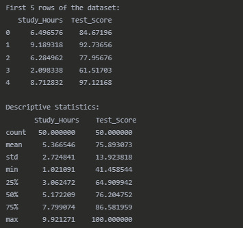
print("First 5 rows of the dataset:") print(df.head())

#Calculate descriptive statistics

print("\nDescriptive Statistics:") print(df.describe())

#Calculate Pearson correlation coefficient

r, p_value = stats.pearsonr(df['Study_Hours'], df['Test_Score']) print("\nPearson Correlation Results:") print(f"Correlation coefficient (r): {r:.4f}") print(f"P-value: {p_value:.4f}") print(f"Coefficient of determination (r²): {r**2:.4f}")

#Create a scatter plot with regression line

plt.figure(figsize=(10, 6)) sns.regplot(x='Study_Hours', y='Test_Score', data=df, line_kws={"color":"red"}) plt.title('Relationship Between Study Hours and Test Scores') plt.xlabel('Study Hours') plt.ylabel('Test Score') plt.grid(True, linestyle='--', alpha=0.7)

#Add correlation coefficient text to the plot

plt.text(1.5, 90, f'r = {r:.4f}', fontsize=12) plt.text(1.5, 85, f'r² = {r**2:.4f}', fontsize=12) plt.text(1.5, 80, f'p-value = {p_value:.4f}', fontsize=12)

plt.tight_layout() plt.show()

#Check if the correlation is statistically significant

alpha = 0.05 if p_value < alpha: significance = "statistically significant" else: significance = "not statistically significant"

print(f"\nThe correlation between study hours and test scores is {significance} at the {alpha} level.")

#Interpret the strength of the correlation

if abs(r) < 0.3: strength = "weak" elif abs(r) < 0.7: strength = "moderate" else: strength = "strong"

print(f"The correlation coefficient of {r:.4f} indicates a {strength} positive relationship.") print(f"The coefficient of determination (r²) of {r2:.4f} suggests that {(r2 * 100):.2f}% of the") print(f"variation in test scores can be explained by variation in study hours.")

Results

Dataset Overview

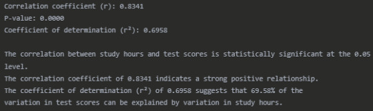
Pearson Correlation Results

Interpretation

The Pearson correlation analysis reveals a strong positive relationship (r = 0.8341) between the number of hours students spend studying and their test scores. This correlation is statistically significant (p < 0.0001), indicating that the relationship observed is unlikely to have occurred by chance.

The scatter plot visually confirms this strong positive association, with students who study more hours generally achieving higher test scores. The regression line shows the overall trend of this relationship.

The coefficient of determination (r² = 0.6958) tells us that approximately 69.58% of the variability in test scores can be explained by differences in study hours. This suggests that study time is an important factor in determining test performance, although other factors not measured in this analysis account for the remaining 30.42% of the variation.

These findings have practical implications for students and educators. They support the conventional wisdom that increased study time generally leads to better academic performance. However, the presence of unexplained variance suggests that other factors such as study quality, prior knowledge, learning environment, or individual learning styles may also play significant roles in determining test outcomes.

Conclusion

This analysis demonstrates a strong, statistically significant positive correlation between study hours and test scores. The substantial coefficient of determination suggests that encouraging students to allocate more time to studying could be an effective strategy for improving academic performance, though it's not the only factor that matters. Future research could explore additional variables that might contribute to the unexplained variance in test scores.

[ryhanpz]

Exploring the Link Between Income and Life Expectancy: A Pearson Correlation Analysis

This blog post explores the relationship between income per person and life expectancy using data from the Gapminder Project. With global development and public health being major concerns, understanding how wealth relates to health outcomes—such as how long people live—is critical for researchers and policymakers alike. This analysis uses Pearson correlation to examine whether countries with higher income levels also tend to have longer average life expectancies.

The Dataset: Gapminder

The dataset used in this analysis is part of the Gapminder Project, a comprehensive resource offering statistics on health, wealth, and development indicators from countries around the world.

For this analysis, we focus on two numerical variables:

Income per Person: 2010 Gross Domestic Product per capita in constant 2000 US$. The inflation but not the differences in the cost of living between countries has been taken into account.

Life Expectancy: 2011 life expectancy at birth (years). The average number of years a newborn child would live if current mortality patterns were to stay the same

These two continuous variables are ideal for evaluating a linear association using Pearson correlation.

The Code: Pearson Correlation in Action

import pandas import numpy import seaborn import scipy import matplotlib.pyplot as plt

data = pandas.read_csv('gapminder.csv', low_memory=False)

# Convert variables to numeric

data['incomeperperson'] = pandas.to_numeric(data['incomeperperson'], errors='coerce') data['lifeexpectancy'] = pandas.to_numeric(data['lifeexpectancy'], errors='coerce')

# replace empty strings or spaces with NaN if needed

data['incomeperperson'] = data['incomeperperson'].replace(' ', numpy.nan) data['lifeexpectancy'] = data['lifeexpectancy'].replace(' ', numpy.nan)

# Drop missing values

data_clean = data.dropna(subset=['incomeperperson', 'lifeexpectancy'])

# Scatterplot

scat = seaborn.regplot(x="incomeperperson", y="lifeexpectancy", fit_reg=True, data=data_clean) plt.xlabel('Income per Person') plt.ylabel('Life Expectancy') plt.title('Scatterplot: Income per Person vs. Life Expectancy ')

# Pearson correlation

print('Association between income per person and Life Expectancy:') print(scipy.stats.pearsonr(data_clean['incomeperperson'], data_clean['lifeexpectancy']))

Interpreting the Results

The scatterplot visually shows the relationship between income and life expectancy, with a regression line representing the trend. A positive slope suggests that as income per person increases, so does life expectancy. The Pearson correlation coefficient (r) and p-value are printed. Here's how to interpret them:

r ranges from -1 to +1.

If r > 0, the relationship is positive.

If r < 0, the relationship is negative.

If r ≈ 0, there's little to no linear relationship.

The p-value tests the statistical significance of the correlation.

If p < 0.05, the correlation is statistically significant.

Correlation coefficient (r) = 0.60: This indicates a moderate to strong positive correlation. As income per person increases, life expectancy generally increases as well.

p-value ≈ 1.07e-18: This value is far below 0.05, which means the result is statistically significant. We can confidently reject the null hypothesis and say that there's a significant linear association between income and life expectancy.

[nursingwriter]

Ramos Article Critique Problem Statement The study by Ramos (2023) was performed to gain more understanding of the relationship between planned behavior (TPB) and self-determination theory (SDT) in terms of health-seeking behavior among older adults who are dealing with hearing loss. The author frames the problem by stating that in spite of the prevalence of hearing impairment in older adults, many do not seek medical help. The purpose of the study is to examine how TPB and SDT can improve health-seeking behaviors for this target population. Background/Literature Review Ramos (2023) gives numerous and ample citations for the discussion on TPB, SDT, and health-seeking behavior among older adults. The review of relevant literature gives the reader enough context to understand the need for the study. There are, for example, several references to studies on the effectiveness of TPB and SDT in predicting health behaviors. This is done to show an existing gap in research related to hearing impairment that Ramos (2023) wants to fill. Research Question The research question is never explicitly stated but is inherent in the statement that the study wants to better understand the association between hearing health-seeking intention, motivation, and actual behavior among the older adult population (Ramos, 2023, p. 2). Variables and Hypothesis The independent variables in the study were knowledge competence, relatedness, attitudes, stigma, and perceived competence and autonomy. The dependent variable is health-seeking behavior. The research hypothesis is that the constructs of TPB and SDT, such as knowledge competence, relatedness, positive attitudes towards hearing loss, lower stigma levels, and perceived competence and autonomy, maybe significant predictors that influence health-seeking behavior among older adults with hearing impairment (Ramos, 2023, p. 2). Design Ramos (2023) used a prospective correlational design to examine the factors associated with hearing health-seeking behavior, as this design supports identifying relationships. Sample/Ethics/Setting A convenience sample of 103 community-dwelling older adults was recruited from churches and senior centers. However, there is no evidence that participants' rights were protected via informed consent or confidentiality measures. Ramos (2023) does note that Institutional Review Board approval was sought, though. Procedure Ramos (2023) recruited participants, conducted initial hearing screenings, administered questionnaires, and conducted follow-up interviews eight weeks later to gain data about whether participants sought medical help for their hearing loss. Data was collected via reliable instruments: Attitudes toward Loss of Hearing Questionnaire, Hearing Attitudes Rehabilitation Questionnaire, and Perceived Competence Scale, which showed acceptable internal consistency with Cronbachs alpha coefficients ranging from 0.61 to 0.92 (Ramos, 2023, p. 2-3). Analysis Data were analyzed using descriptive statistics, Pearsons correlations, and regression analyses, suitable for exploring relationships between variables and making predictions. The use of multiple regression analyses contributed to the goal to better understand TPB and SDT constructs as they related to the subjects intention to seek medical help for their hearing. Results Ramos (2023) found that the more an older adult possessed knowledge competence, relatedness, positive attitudes, and perceived competence and autonomy the more likely he was to seek medical help for hearing loss. The reported results show internal validity, since they are supported by the theoretical framework and what prior research has shown. Qualitative Content The study used a quantitative design; there was no indication of qualitative research being conducted. Ramos (2023) did identify limitations, such as small sample size and the studys reliance on self-reported data, which is always subject to bias. Ramos (2023) stated that future research may want to look at using longitudinal or experimental designs to understand the complex interplay between the variables better (Ramos, 2023, p. 6). References Ramos, M. D. (2023). Exploring the relationship between planned behavior and self- determination theory on health-seeking behavior among older adults with hearing impairment.Geriatric Nursing,52, 1-7. https://www.paperdue.com/customer/paper/knowledge-competence-intentions-seek-medical-2181912#:~:text=Logout-,KnowledgeCompetenceIntentionsSeekMedical,-Length2pages   Read the full article

[literaturereviewhelp]

A Pearson correlation coefficient was conducted to determine the relationship between the dependent and the independent variables. This chapter thus will highlight the analysis results and bring them to perspective. Correlation analysis Testing hypotheses H1. Four factors (Price, genre, tweets, and frequency of tweets) and VOD booking have positive correlation The hypothesis test whether the four factors (Price, genre, tweets, frequency of tweets) and VOD booking have related positively The results of a regression analysis show that the four factors together predict VOD booking significantly, F=105.635, p < .001 as illustrated in Table 1. The Second regression analysis results indicate that the three factors (Price, genre, tweets) together predict VOD booking, F=80.389, p < .001 as illustrated in Table 2. The third regression analysis results indicate tweets, which is a technically an advertisement strategy predict VOD booking, F=128.790, p < .001 as illustrated in Table 3. This is explained by the fact that the Social Media Analytics asserts the intersections of social network including twitter and business at large. Moreover, it has focused more on dynamic capabilities, awareness motivation, organizational benefits and information technology resources (Yeates, 2002). Table 1: ANOVAb Model Sum of Squares df Mean Square F Sig. 1 Regression 21.981 1 21.981 105.635 .000a Residual 19.768 95 .208 Total 41.749 96 a. Predictors: (Constant), four factors (Price, genre, tweets, frequency of tweets) b. Dependent Variable: mean VOD booking Table 2: ANOVAb Model Sum of Squares df Mean Square F Sig. 1 Regression 19.135 1 19.135 80.389 .000a Residual 22.613 95 .238 Total 41.749 96 a. Predictors: (Constant), three factors (Price, genre, tweets,) b. Dependent Variable: VOD booking Table 3: ANOVAb Model Sum of Squares df Mean Square F Sig. 1 Regression 24.026 1 24.026 128.790 .000a Residual 17.723 95 .187 Total 41.749 96 a. Predictors: (Constant), tweets b. Dependent Variable: mean VOD booking Table 4 shows regression analysis results comparing three items including three factirs, four factors, and number of tweets. The four senses (feel, think, sense, act) together predict customer satisfaction, F=80.389. Four factors (Price, genre, tweets, frequency of tweets,) together predict VOD booking, F=105.635. Number of tweets predict VOD booking, F=128.790. The F values of the regression analysis indicate that number of tweets had a higher positive correlation as compared to four factors to VOD bookings. There was a significant affirmation that the number of tweets influenced the number of bookings of the video on demand. According to Kaplan & Haenlein (2010), social media has contributed largely toward customer’s perceptions and attitude on products and services. Social media has provided organizations with a variety of opportunities. In terms of marketing, social media has been in the forefront in cutting marketing cost, and this leads to a higher profit margin. The results is further asserted by the fact thet Tweeter is seen to be in the front position in transmitting information on world happening. Read the full article

[suninblogs]

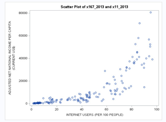
Analysis of Macroeconomic indicators affecting GDP per capita

Preliminary statistical analysis:

Results

Descriptive statistics: descriptive statistics of all the predictor variables under the study and the target variable. The statistics obtained is after data cleaning.

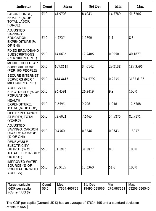
Bivariate analysis :Scatter plots are visualized to understand the association between individual quantitative predictor variables and GDP Per Capita,(Current US$) .Pearson correlation “r” values were calculated for the associations. The Adjusted Net Income Per Capita has the highest r value 0.997289 and p value= 9.550028e-62 which is close to 0.

Lasso regression analysis:

Using Lasso regression analysis, out of 24 predictor variables only 5 strongest predictor variables are retained in the model. The retained variables are:

ADJUSTED NET NATIONAL INCOME PER CAPITA (CURRENT US$)

GROSS DOMESTIC SAVINGS (% OF GDP)

EXPORTS OF GOODS AND SERVICES (% OF GDP)

SECURE INTERNET SERVERS (PER 1 MILLION PEOPLE)

ADJUSTED SAVINGS: EDUCATION EXPENDITURE (% OF GNI)

and rest of the predictor variables are eliminated as they remain insignificant and are shrunk to 0.0 after Lasso regression.

Initially prior to Lasso regression it is observed that Personal Remittance paid had the highest mean but post Lasso regression this variable is shrunk to 0. Lasso doesn’t just look at raw coefficients, it balances predictive accuracy with sparsity. It selectively shrinks coefficients based on their relative importance in explaining the variance of the dependent variable.  If the high-mean variable is not strongly predictive (i.e., it is highly correlated with other predictors or adds little unique information), Lasso may shrink its coefficient aggressively.

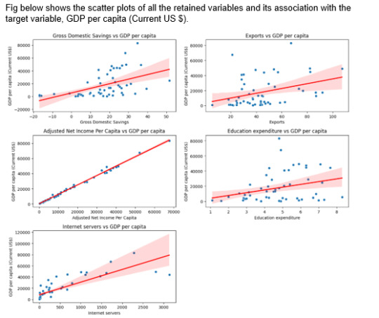
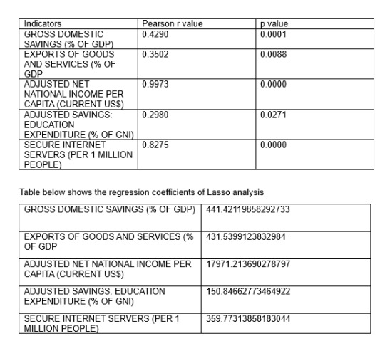
The strongest predictors are Adjusted Net National Income Per Capita (Current US$) followed by Gross Domestic Savings (% of GDP) and so on. Hence, these are the most significant predictors that have a positive influence on GDP per capita and help boost the nation’s economy.

Together, these 5 predictors accounted for 99.4 % accuracy in the training set and 99.5% accuracy in test set. Also, the mean squared error (MSE) for the test data (MSE= 2769007.811 differed slightly from the MSE for the training data (MSE= 1520763.18).

[williambaker19]

Title: Exploring the Moderating Effect of Latitude on the Depth-Diameter Relationship in Martian Craters

IntroductionIn planetary geology, crater characteristics such as depth and diameter provide insights into impact dynamics and surface evolution. This analysis explores whether latitude moderates the correlation between crater depth and diameter. If latitude plays a significant role, we expect the relationship between depth and diameter to differ across latitudinal groups.

MethodologyWe use the Mars crater dataset and employ Pearson’s correlation coefficient to analyze the relationship between crater depth and diameter across different latitude groups. We define latitude groups using median-split quantiles, dividing the dataset into "Low" and "High" latitude categories.

Statistical Analysis Syntax (Python Code)

Results

Low Latitude Group:

Correlation between crater diameter and depth: 0.589

p-value: 0.000 (statistically significant)

High Latitude Group:

Correlation between crater diameter and depth: 0.590

p-value: 0.000 (statistically significant)

InterpretationThe correlation between crater diameter and depth is strong and statistically significant in both latitude groups. However, the correlation values are nearly identical (0.589 vs. 0.590), suggesting that latitude does not meaningfully moderate this relationship. This implies that the depth-diameter association is consistent across different latitudinal zones on Mars.

ConclusionThis study tested whether latitude acts as a moderator in the depth-diameter relationship of Martian craters. The findings indicate that latitude does not significantly alter the correlation, implying that other factors—such as impactor properties or surface composition—may play a more prominent role. Future research could explore additional moderators, such as crater age or surface material properties, to gain deeper insights into crater formation processes.

[assignmentwriterssrilanka]

 SPSS Statistical Analysis: A Comprehensive Overview

Statistical analysis is a cornerstone of research and data interpretation across various disciplines. One of the most widely used statistical software packages for this purpose is SPSS (Statistical Package for the Social Sciences). In this article, we will explore some fundamental concepts involved in statistical analysis using SPSS, including validity,reliability, descriptive statistics, correlation, and multiple regression.

Validity

Validity refers to the accuracy and relevance of the findings derived from a statistical analysis. In the context of SPSS, a study is said to be valid if the conclusions drawn from the data accurately represent the true relationships and phenomena being investigated. There are several types of validity, including:

Construct Validity: Ensures that the test truly measures the construct it purports to measure.

Content Validity: Assesses whether the measurement encompasses the full domain of the intended variable.

Criterion-related Validity: Examines how well one measure predicts an outcome based on another measure.

In using SPSS, researchers can conduct various tests to check for validity, such as factor analysis, which helps ensure that the factors used in your study genuinely represent the underlying constructs.

Reliability

Reliability refers to the consistency of a measure. A reliable instrument will yield the same results when applied to similar populations under similar circumstances. In SPSS, researchers assess reliability using several statistical techniques:

Cronbach's Alpha: A common measure for internal consistency of a scale. Values above 0.70 typically indicate acceptable reliability.

Test-Retest Reliability: Compares scores from the same subjects at different times to assess stability over time.

Inter-Rater Reliability: Assesses the degree of agreement among different raters or observers.

Reliability is crucial in ensuring that the data collected through SPSS is trustworthy and repeatable.

Descriptive Statistics

Descriptive statistics provide a summary of the data and include measures such as mean, median, mode, and standard deviation. SPSS offers a range of options to easily calculate these values, allowing researchers to gain a quick understanding of their data sets. Key points in descriptive statistics include:

Central Tendency: Measures (mean, median, mode) that provide insights into the average or most common values.

Dispersion: Measures (range, variance, standard deviation) that describe the spread of data points in the sample.

Frequency Distributions: Visual representations like histograms or bar charts that summarize data occurrences.

Using descriptive statistics in SPSS helps researchers distill complex data into manageable summaries, making it easier to identify trends and patterns.

Correlation

Correlation analysis in SPSS allows researchers to explore the relationships between variables. It quantifies the degree to which two variables are related, using correlation coefficients (such as Pearson’s r). Key aspects include:

Positive Correlation: Indicates that as one variable increases, the other tends to increase.

Negative Correlation: Indicates that as one variable increases, the other tends to decrease.

No Correlation: Suggests no relationship exists between the two variables.

SPSS provides tools to create scatter plots and calculate correlation coefficients, offering visual and numerical insights into the relationships being studied.

Multiple Regression

Multiple regression analysis extends correlation by allowing researchers to examine the predictive relationship between one dependent variable and multiple independent variables. It is an essential technique for understanding complex relationships. Key points include:

Model Fitting: Multiple regression helps researchers fit a model that describes the relationship between variables, determining how much variance in the dependent variable can be explained by the independent variables.

Coefficients Interpretation: The output from SPSS provides regression coefficients that indicate the nature and strength of the relationship of each independent variable with the dependent variable.

Assumptions Checking: Before interpreting results, it is crucial to check assumptions (such as linearity, independence, homoscedasticity, and normality of residuals) to ensure valid inferences.

Multiple regression in SPSS thus offers a powerful mechanism to identify and quantify complex relationships among variables, supporting informed decision-making based on statistical evidence.

Conclusion

SPSS is an invaluable tool for conducting statisticalanalysis, offering a robust platform for evaluating validity, reliability, descriptive statistics, correlation, and multiple regression. Mastery of these concepts enhances the effectiveness of data analysis and enriches the research process, allowing for informed conclusions and evidence-based decisions. With this knowledge, researchers can leverage SPSS to its fullest potential, transforming data into actionable insights.

[sidslash918]

Milestone Assignment 3: Preliminary Results

1. Preliminary Statistical Analyses

This study investigates the relationship between Adjusted Net National Income Per Capita (Current US$) and various socio-economic indicators using data from the World Bank (2013). The goal is to analyze trends and correlations to determine the most influential factors affecting a nation's economic well-being.

Statistical Approaches Used

The statistical analyses included:

Descriptive Statistics: Summary statistics for each variable (mean, standard deviation, range, etc.).

Correlation Analysis: Pearson correlation coefficients to assess relationships between Adjusted Net National Income Per Capita and independent variables.

Distribution Analysis: Evaluating data normality through histograms, Q-Q plots, and goodness-of-fit tests.

Scatter Plots: Visualizing linear relationships between selected economic indicators and national income.

Box Plots: Comparing variations in Adjusted Net National Income Per Capita across different socio-economic levels.

Key Findings from Bivariate Analysis

Descriptive Statistics

The mean Adjusted Net National Income Per Capita was $12,299, with a standard deviation of $16,046, indicating significant variability across countries. The median value was $5,300, highlighting a skewed distribution with several high-income outliers. The highest recorded value was $80,588, while the lowest was $154.

Key Summary Statistics for Adjusted Net National Income Per Capita:

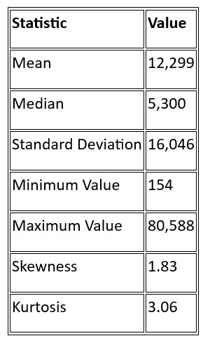
The skewness value of 1.83 suggests that the data is positively skewed, meaning most countries have lower values of Adjusted Net National Income Per Capita, with a few outliers pulling the mean upwards.

Correlation Analysis

The correlation analysis was conducted between Adjusted Net National Income Per Capita and several socio-economic indicators. The key relationships observed were:

A strong positive correlation (r = 0.84) was observed between Fixed Broadband Subscriptions and Adjusted Net National Income Per Capita, suggesting that technological penetration is a major driver of economic prosperity. Similarly, Internet Users had a strong correlation (r = 0.81), reinforcing the impact of digital access on national income levels.

However, Female Labor Force Participation showed a weak correlation (r = 0.08), suggesting that labor force composition alone does not significantly influence national income.

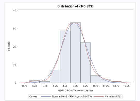
Distribution Analysis

A Q-Q plot for GDP Growth indicated a near-normal distribution, with a mean GDP growth rate of 3.44% and a standard deviation of 3.00%.

The Food Production Index followed a slightly right-skewed distribution, with a mean of 121.29 and standard deviation of 21.41.

Histogram of Adjusted Net National Income Per Capita

The distribution of Adjusted Net National Income Per Capita showed significant right skewness, confirming that most countries have lower income levels, with a small number of high-income outliers.

Graphical Representation of Results

Below are visual representations of key relationships observed in the analysis:

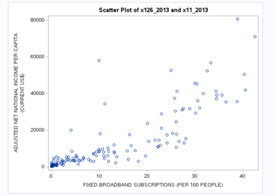
Scatter Plot - Broadband Subscriptions vs. Adjusted Net National Income Per Capita

A strong positive correlation (r = 0.84) was observed between Fixed Broadband Subscriptions per 100 people and Adjusted Net National Income Per Capita, confirming the importance of technology in economic growth.

Scatter Plot - Health Expenditure vs. Adjusted Net National Income Per Capita

A moderate positive correlation (r = 0.53) was found between Health Expenditure as % of GDP and Adjusted Net National Income Per Capita, suggesting that greater investments in healthcare are associated with higher economic development.

Scatter Plot - Internet Users vs. Adjusted Net National Income Per Capita

A strong positive relationship (r = 0.81) was observed between Internet Penetration and Adjusted Net National Income Per Capita, highlighting the role of digital access in improving national income levels.

Conclusion

The preliminary statistical analysis confirms that technology penetration (broadband subscriptions, internet access), urbanization, and infrastructure (sanitation, health expenditure) are strongly associated with higher Adjusted Net National Income Per Capita.

[bbadland]

Assignment 5

Question A.

A1: The null hypothesis, or H(0), is that the machine is working correctly with a mean breaking strength of 70lbs. The alternative hypothesis, or H(A), is that the machine is not working correctly, and the mean breaking strength is a different value than 70lbs. 

A2: Using a 0.05 level of significance, we fail to reject H(0), as the p-value is 0.072. Therefore, there is no evidence that the machine is not meeting manufacturer specifications. 

A3: The p-value is 0.072, which is greater than 0.05, leading us to fail to reject H(0). This means that the probability of the result occurring by chance is 7.2%. In order to reject H(0), we would need a statistically significant result below 0.05. 

A4: If the standard deviation was 1.75, we would reject the null hypothesis, as the p-value would be below 0.05. This would mean that there is statistically significant evidence that the machine is not meeting manufacturer specifications.

A5: If the sample mean were just slightly lower at 69lbs and the standard deviation remaining at 3.5lbs, we would reject the null hypothesis. The p-value becomes 0.045, giving statistically significant evidence that the machine is not meeting manufacturer specifications. 

Question B.

The 95% confidence interval estimate is from 83.04 to 86.96.

Question C.

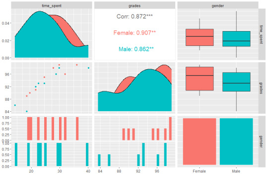
C1: Pearson’s correlation coefficient between time spent studying to grades is 0.91 for girls and 0.86 for boys.

C2: