mysteriousquantumphysics

[mysteriousquantumphysics]

Happy Pi Day 2025!

Happy Pi Day 2023!

[mysteriousquantumphysics]

Circuit Cutting for Efficient Quantum Circuit Simulation

In previous blog posts [1, 2] we talked about quantum circuit cutting - a technique to "cut" quantum circuits into pieces to run them on smaller quantum devices. In particular, for NISQ devices this is a nice method to run larger quantum circuits than usually possible with the limited number of qubits as well as diminishing the effects of noise during the computation [3]. However, such techniques come with the cost of having an exponential sampling overhead in the number of cut wires or gates. Thus, such methods are limited in applicability - namely they work best for shallow, easy to partition, circuits.

"Cutting" for Classical Simulation

No matter the (dis)advantages, the idea of "cutting" circuits into pieces cannot only be applied as a "compilation" step to run cut algorithms on real quantum devices. In contrast, "cutting" can also make classical simulations of quantum circuits of suitable classes more efficient. Why might it be desirable to simulate smaller circuits on a classical computer? The simple answer is that storing statevectors on classical computers requires an exponential amount of RAM, i.e., 2^n amplitudes for n qubits. As only limited RAM is available - similar to the limited number of qubits in NISQ devices - running smaller simulations/computations is desirable. However, there is no free lunch here as well, since cutting also induces an exponential overhead in the classical simulation case - meaning that an exponential amount of smaller subcircuits has to be run and subsequently reassembled again. Thus, the reason why one wants to cut circuits for classical simulations is a bit more intricate: Reducing the RAM requirements can also decrease the runtime of simulating gates (i.e. by matrix-vector multiplication) but as pointed out before, one has to run an exponential amount of circuits which is increasing the time cost again. Therefore, cutting quantum circuits for classical simulation is not always useful; instead, there is a tradeoff between reducing runtime by reducing RAM and the exponential overhead - thus, such techniques are usually only useful for quantum circuits with limited connectivity such that only a manageable number of cuts must be performed. In the literature this cutting is usually denoted as Hybrid Schrödinger Feynman Technique (HSF) [4, 5, 6] - still, the underlying ideas are quite similar to quantum circuit cutting. Let's look at the core idea of cutting circuits for classical simulation and where this aforementioned exponential overhead comes from.

How to Cut Circuits for Simulation

Conceptually, classical cutting of quantum gates (contrasting quantum circuit cutting, one is usually not considering wire cuts for HSF simulation) merely requires performing a Schmidt-Decomposition on the gate(s) to be cut. Considering the CNOT gate, this can be done quite easily by just factoring out properly as follows

where we just wrote down the CNOT gate in Dirac notation and factored out the projector P_0 and P_1 respectively. This can be represented graphically in a circuit diagram as

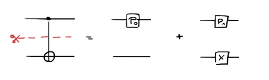
With this illustration it becomes more apparent what is meant by cutting. We decomposed the CNOT gate, which originally acts on two qubits jointly, into a representation with two contributions (terms) in which each one is bipartite: The first term is just the projector onto the zero state on the first qubit and nothing on the other. The second term is the projector onto the other computational basis state as well as a separate Pauli X gate on the other qubit. You can see that the qubit wires are not connected anymore in the separate contributions that constitute the cut.

If you have a larger circuit that you want to partition into two smaller parts which should be simulated separately and they are connected by a single CNOT gate, cutting would give you two pairs of bipartite circuits. Each of them is smaller than before, thus, faster to simulate. This toy example has a pretty small overhead in the number of simulations, often also denoted as "paths", namely only two. If more gates are cut, this grows exponentially as the number of paths per gate has to be multiplied. Mathematically speaking, this number of paths is determined by the Schmidt-rank of each cut gate. As mentioned before, the Schmidt Decomposition is the core tool to perform cutting and thus, we briefly look into how this Schmidt Decomposition is done in general.

Classical Cutting in General by Schmidt-Decompositions

In order to spare you tedious notation with a lot of confusing indices, let's consider the general case in graphical notation only. Any quantum circuit can be represented as a tensor network [7]. Each quantum wire can be interpreted as leg of a tensor with physical dimension 2 (since qubits have a basis with 2 vectors). Consider some operator A with n=6 qubits (the logic applies for arbitrarily many qubits) as shown in the figure below. Assume that we want to cut this operator in the middle. Originally, operator A has 2n legs , but we can reshape those legs/wires according to the desired cut location as shown on the right-hand side - resulting in two "big" legs with higher dimensions than before. The dimension of the upper and lower big leg is determined by the number of qubits n_a in the upper partition and n_b in the lower partition respectively, in our example n_a=n_b=3. The upper big leg has dimension 2^(2n_a) and the lower 2^(2n_b).

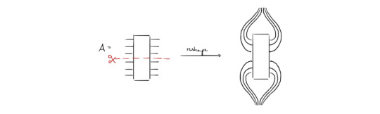
Doing this not only fixes the cut position but is a way of matricizing the previously higher rank object - allowing to perform a Singular Value Decomposition (SVD), which can be applied on matrices (having 2 legs) only. An SVD decomposes a matrix into three parts, two isometries, U and V as well as the diagonal matrix σ containing the singular values (shown diagramatically below). The number of singular values fixes the aforementioned Schmidt-rank [8] of the original operator/gate A which, in turn, determines the aforementioned overhead, the number of paths in the simulation. The isometries can be absorbed into the top and bottom and the remaining sum can be made explicit such that we end up with a bipartite representation, similar to the one shown for the CNOT gate. This allows to decompose the gate into two parts, at the cost of a higher number of paths for the simulation.

Conclusion

Now you know how circuit cutting can be applied for classical simulations as well - it merely requires performing a Schmidt Decomposition in order to find bipartite representations of gates to be cut. Interestingly, performing cuts for classical simulation induces an exponential overhead - similar to quantum circuit cutting for real quantum devices. Even though conceptual differences are present between both approaches, this parallel neatly shows that one can never avoid the exponential complexity of quantum systems: We can merely shift the complexity (e.g. memory complexity into time complexity as for HSF simulation), to hope for nice tradeoffs and computing advantages - but no method can get rid of the inherent exponential complexity of quantum systems.

References

[1] Blog Post "Cutting Quantum Circuits into Pieces - Why and How?"

[2] Blog Post "Quantum Circuit Cutting - with Randomly Applied Channels"

[3] Bechtold, M., Barzen, J., Leymann, F., Mandl, A., Obst, J., Truger, F., & Weder, B. (2023). Investigating the effect of circuit cutting in QAOA for the MaxCut problem on NISQ devices. In Quantum Science and Technology (Vol. 8, Issue 4, p. 045022). IOP Publishing. https://doi.org/10.1088/2058-9565/acf59c

[4] Aaronson, S., & Chen, L. (2016). Complexity-Theoretic Foundations of Quantum Supremacy Experiments (Version 2). arXiv. https://doi.org/10.48550/ARXIV.1612.05903

[5] Markov, I. L., Fatima, A., Isakov, S. V., & Boixo, S. (2018). Quantum Supremacy Is Both Closer and Farther than It Appears. arXiv. https://doi.org/10.48550/ARXIV.1807.10749

[6] Burgholzer, L., Bauer, H., & Wille, R. (2021). Hybrid Schrödinger-Feynman Simulation of Quantum Circuits With Decision Diagrams. In 2021 IEEE International Conference on Quantum Computing and Engineering (QCE). 2021 IEEE International Conference on Quantum Computing and Engineering (QCE). IEEE. https://doi.org/10.1109/qce52317.2021.00037

[7] Blog Entry Pennylane, "Tensor Network Quantum Circuits"

[8] Nielsen, M. A., Dawson, C. M., Dodd, J. L., Gilchrist, A., Mortimer, D., Osborne, T. J., Bremner, M. J., Harrow, A. W., & Hines, A. (2003). Quantum dynamics as a physical resource. In Physical Review A (Vol. 67, Issue 5). American Physical Society (APS). https://doi.org/10.1103/physreva.67.052301

[mysteriousquantumphysics]

Updates from my Quantum Journey

It's been silent on my blog for a while now - the past year has been a busy time for me since I was working on my Master's thesis as well as working as a research assistant at Fraunhofer in parallel. Both were great experiences but it became so time-consuming that I totally lost track of posting any content on this blog!

In April 24 I finished my Master's Thesis in Physics in which I was mainly working on tensor networks. We tried to make DMRG (Density Matrix Renormalization Group) for Quantum Chemistry-like setups more efficient by lifting degeneracies in the symmetry sectors of the tensor network structure. Besides from what I learned on the physics-side of this project, it helped me to foster my fascination for method-development.

My work at Fraunhofer was very rewarding as well - I did not only learn a lot, I also had the chance to contribute in two publications in the area of quantum circuit cutting. In case you are interested, I could write a blog entry for one or both of the papers(:

During all this hard work and (to be honest) frustration and exhaustion in the past year I had this optimistic hope of doing a PhD after finishing my Master's degree. Now, this dream has become a reality and I started my PhD at the Technical University of Munich this month. I am really grateful for this oppurtunity in which I can work full-depth in the field of quantum computing - with a strong focus on software/method development. I am excited about what this journey has to offer and I am very much looking forward to it!

[mysteriousquantumphysics]

Happy Pi Day 2024!

Happy Pi Day 2023!

[mysteriousquantumphysics]

How to Use Quantum Computing as a Tool for Philosophy of Science

Recently, I attended the MCQST 2023 Conference on which Lídia del Rio presented the research with her collaborators about quantum thought experiments in a quantum computer. They wrote a whole package to do this and describe the ideas in detail in [1]. It's definitely worth checking out the paper and the package - to make you curious let us look at an illustrative example [1, p.4-10].

Example Setting

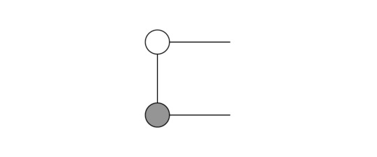
Let us consider the following setting (as depicted in the image above): Alice has some two-level quantum system R (e.g. a qubit) in the state written in blue. Thus, the probability of obtaining a=0 in a measurement is 1/3 while the result a=1 will be obtained with a probability 2/3. Depending on the outcome, Bob receives the a system in state |0> (if Alice's result was a=0) or in state |+> ~ |0>+|1> (if Alice's result was a=1). In turn, Bob measures his system in the computational basis and can receive the outcome b=0 or b=1. What conclusions can Bob draw about Alice's measurement outcomes based on his? It is assumed that Bob knows the rules upon which Alice sends him the different systems. Thus, if his outcome is b=0 he cannot make any retrodiction since the outcome b=0 could stem from both possible states |0> and |+>. However, if he measures b=1 he knows that his state must have been in |+> and thus he can retrodict that Alice's outcome must have been a=1. Therefore, in one of both cases Bob can draw a deterministic conclusion about Alice's outcome.

So far so good, at this point I'd like to mention that even though this setup seems to be motivated by the Frauchiger-Renner Thought Experiment, we will not talk about apparent paradoxes or fundamental questions in foundations of quantum mechanics themselves. Instead the setting is supposed to be easy to grasp and can therefore neatly serve the purpose to illustrate how a thought experiment can be formalized in terms of quantum circuits. Hence, we will discuss a tool which can be used for quantum thought experiments in general by using a simple example.

Alice's and Bob's Brains in a Quantum Circuit

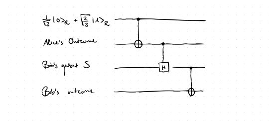
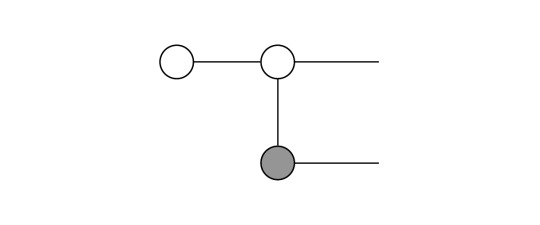
Next, we will translate this specific setting as a quantum circuit - by going through the above illustration of the resulting circuit. The first qubit is initialized in the state of Alice's system R. Even though this seems to be the only true quantum system at hand, we will act as if there was an external observer who looks at both Alice and Bob and their respective systems. Imagine you are in the position of this external observer and set the Heisenberg cut at this point: You are classical while both Alice and Bob are quantum (as it is done in Neo-Copenhagen interpretations). Then, one also has to model the "brains"/"memory" of both Alice and Bob. We start with Alice first: we assign a wire of the circuit to Alice's reasoning which basically means that somehow the possible measurement results are stored in this respective qubit. The wire representing her memory is initialized in state |0> and is connected to her system R via a CNOT gate. This means that if the system R was in state |0>, the qubit representing Alices would stay in |0>. However, if R was in |1>, Alice's state of memory would be in |1> as well. This way, one can model different measurement outcomes and also Alice's memory in a unitary manner without explicitly including measurements in the circuits yet. This is necessary since from our external perspective everything about Bob and Alice is considered to be quantum, i.e. must be modelled unitarily. Now, we can look at the third wire: It is again initialized in state |0> and remains in this state if Alice's memory is in state |0>. However, the controlled Hadamard will act on the third wire if Alice's memory is in state |1>, hence it would be turned into state |+>. Thus the controlled Hadamard models the system S which Bob receives - conditioned on Alice's measurement outcome of R. Finally, the last wire is again initialized in |0> and is supposed to model Bob's memory. Exactly as Alice's memory, also the relation between Bob's memory and his system S is modeled via a CNOT gate.

As a result we now have a quantum circuit which represents the setup from above from an external perspective. I think already at this point one can see the beauty of this approach - while one needs quite a lot of sentences to explain the simple setup, it can very easily be grasped by the neat quantum circuit. What is left to do now is to model Bob's reasoning regarding his retrodiction on Alice's outcome. We found that Bob can draw a deterministic conclusion about Alice's measurement outcome if his outcome is b=1, in the other case he cannot draw such a conclusion. How can this be mapped into a quantum circuit?

Modelling Bob's reasoning

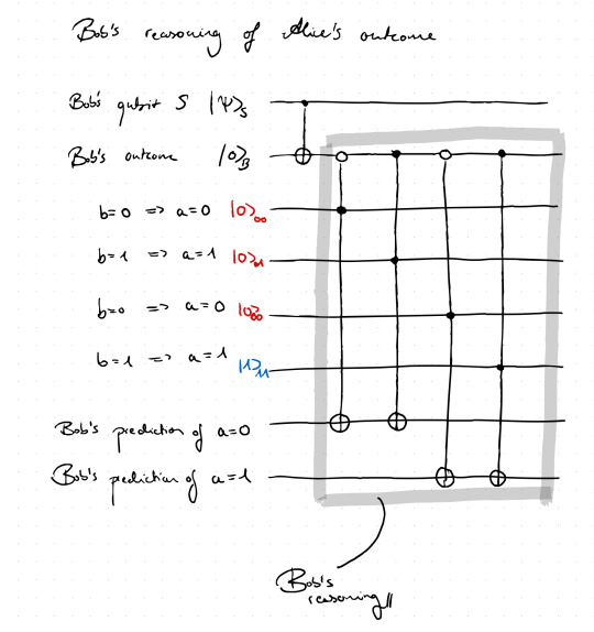
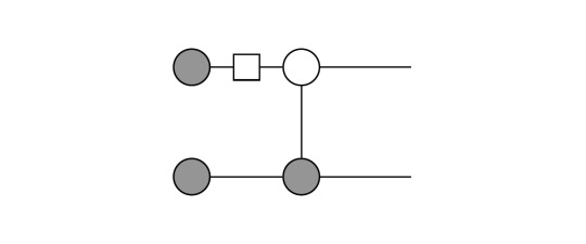
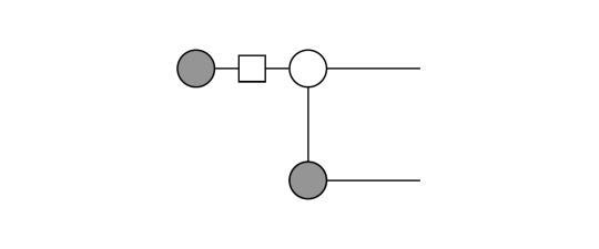
In the above circuit we added a couple of additional wires. One set represents the four possible logical inferences in this case, and the last two wires will show what Bob's prediction will be based on the initialized inferences. Let's go through this step by step: There are four possible inferences on the measurement outcomes a and b, but only one of them is assumed to hold, namely (b = 1 -> a=1), which is why only the wire corresponding to this inference is initialized in state |1>. The other three inferences, which are assumed not to hold, are initialized in |0> and since there are control nodes from the nonlocal Toffoli-type on those wires, they will not really contribute as long as one does not change the initialization. Those Toffoli-type gates have two control nodes each as well as a NOT at the lower end. One control node is placed on Bob's memory qubit, acting dependently on the outcome b and represents the antecedent of each possible inference. If the inference of a wire assumes b=1 the corresponding Toffoli node on Bob's memory will be black, while it will be white for b=0. The second control node of each Toffoli gate is black in order to be activated according to which inference is initialized with state |1>. The consequent of those inferences is modeled by the lowest two wires. The NOT of each Toffoli is placed on the corresponding wires representing the consequent. Looking at the Toffoli for the inference b=1 -> a=1, one can see that if Bob's memory is in |1> and simultaneously the wire of the corresponding inference is initialized as |1> as well, the NOT on the lowest wire will turn the respective state to |1> (the prediction wires are initialized in |0>). Thus, Bob's prediction can be read off by the states of the prediction wires. Finally, one can also run this circuit and check its consistency - how?

Consistency Checks

In the above image we have put together all we got so far: Alice's actions from before, as well as bob's actions and his reasoning as discussed right above. The consistency of such a model can be checked by measuring the prediction wires as well as Alice's memory qubit. In this case, the only deterministic inference will show itself if Bob's prediction wire for a=1 will be |1> and this will coincide with Alice's memory being in |1>. For the other case, no inference can be done. This way one can check the consistency of the model and if the results show paradoxical outcomes one knows that something went wrong, that something in the logical reasoning / adopted interpretation of quantum theory is getting problematic. Having everything formalized as a quantum circuit will make the analysis of the issues easier.

Final Remarks

It appears to me that Quantum Circuits are not used here because one expects some computational advantage by running them on a Quantum Computer - instead they are used to neatly formalize subsystems and possible inferences of thought experiments. This way, thought experiments can be made more clear and transparent as well as it is easier to see the problem if the outcomes are not consistent. Therefore, their work shows that quantum circuits have a much broader field of application - it is not only about striving for some kind of quantum advantage for specific decision problems, instead they can also be used to formalize concepts in foundations of quantum mechanics; and this is something I have never thought about before, which is why I am so fascinated by the idea.

---

References: [1] Nurgalieva, Mathis, del Rio, Renner - Thought experiments in a quantum computer. arXiv:2209.06236

[mysteriousquantumphysics]

Quantum Circuit Cutting - with Randomly Applied Channels

Recently, I briefly introduced what circuit cutting is, why it is an advisable thing to do with current quantum hardware (NISQ devices) and what additional costs the cutting is causing. However, I did not go into detail how such a circuit cutting method can look like in detail - this is what this entry will be about. In particular, we will have a look on the circuit cutting procedure proposed by Lowe et. al. [1] in which randomly applied channels are able to cut a circuit.

Identity on Cut Circuits

As mentioned in the previous entry, circuit cutting requires to find a proper identity channel on the cut wires which has reasonably low sampling overhead - the definition of the identity is thus the heart of every circuit cutting procedure. In general, such an identity has the form

where Φ_i is some properly chosen quantum channel. The corresponding cost depends on the value κ

which is the L1 norm of the real coefficients of the identity channel above:

Thus, we see that the main possibility to reduce the sampling overhead is to reduce this value. One possibility with small sampling overhead is the following (however, it is not minimal! The method described in [2] has a lower overhead, but we will not go into detail of this).

The identity channel used in [1] looks like

Here, d=2^k is the dimension of the subspace governing the qubits of the cut. The variable z denotes a Bernoulli random value where z=1 appears with probability d/(2d+1). Later, we will derive this form of the identity channel and will see how this probability and also the expectation E_z emerges. Since, there are two values of z, there are also two quantum channels which can be applied. The first one, Ψ_0, is a measure-and-prepare channel:

The unitaries which are applied on the state prior to measurement have to comprise a 2-design (at least) because otherwise the derivation would not work. Such a design is formed by e.g. Clifford gates but there are many possibilities, one could also rely on approximate designs. Since the form of a quantum channel is not so pictorially, you can see in the following how this channel looks like in "circuit-language":

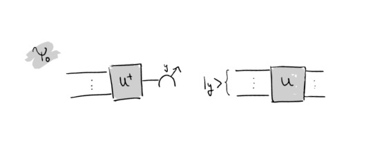
This means, one applies U^\dagger on the k cut wires, measures in z-basis and retrieves a bitstring y. A state in computational basis corresponding to this bitstring gets initialized and then U is applied. All of this is repeated many times. Note that applying such a circuit in the middle of a larger circuit destroys entanglement of the global state and this is also the reason why cutting requires a lot of sampling (quantified by the sampling overhead): The effects of entanglement in the final result must be regained somehow by repeating the procedure numerous times.

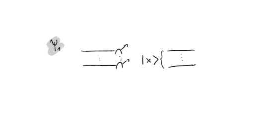
The other channel, Ψ_1, is a simpler one. It is the so-called fully depolarizing channel in which all of the information within the cut (within a sample) is lost:

In practice, the action on the cut part of the circuit is as follows: First one measures the k cut wires in the computational basis. Afterwards one takes a uniformly sampled bitstring x and initializes it on the wires - as in the following circuit snippet:

Guiding through the Derivation

Now, as we have settled the definitions, let's go through the derivation of this identity channel! At first, we need an equation which we shall not prove as this would be more involved (based on Haar measure etc.). It is called Werner Twirling Channel:

This equation is particularly nice because the right hand side is much much simpler than the left hand side, which requires all of the unitaries in the design. At the same time, the right hand side could be quickly written out by hand for e.g. d=1. This will come in handy in deriving the identity channel.

The idea of the proof is to start with one channel Ψ_0 and massage it a little to find an expression of Ψ_1 within it and then massaging it a little further and finding an expression for the identity channel.

Hence, start with the channel Ψ_0:

A lot is going on here, thus let's go through the equalities step by step: From the first to the second line the only thing happening is that we insert an identity (using completeness of the computational basis). Going to the next line, the two scalar factors are swapped and the states with index i can be used to rewrite the expression into a Tr. By exploiting the properties of tensor products and the trace, one can draw outside the sum a partial trace expression in the last line. This shape is nice, because we can recognize the left hand side of the above equation and can simplify the underbraced expression:

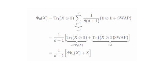
Since the expression within the sum does not depend on the index j anymore, this sum merely gives a factor d. In the second line we draw the partial trace factor into the brackets and recognize the Ψ_1 channel! Additionally, the part with the SWAP operator can be simplified as well (you can easily prove this by checking it with a 4x4 SWAP matrix and using a general matrix X). All of this helped us immensely in relating both channels to each other. Reshaping this equation a little gives us:

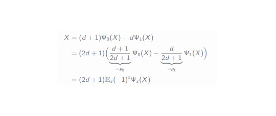
In the second line, we draw a factor outside in order to retrieve the Bernoulli probabilities we have defined previously and then, by respecting the additional sign, this can be easily rewritten as an expectation value in the last line.

What about the cost?

Now as we have both defined and derived the identity circuit expression, let's relate it to the introducing sentences about the sampling overhead. The value of κ can be easily computed:

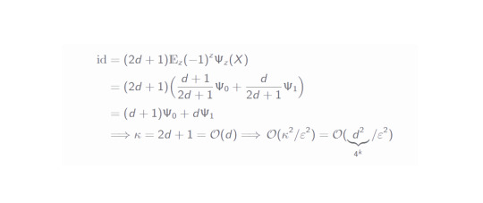
As we can see, the sampling overhead is exponential in the number of cut qubits - this is a deficit in practice. Even though, there are slightly better circuit cutting procedures, the overhead always scales exponentially in the number of cut qubits. Although unfortunate, this makes perfect sense intuitively: The cutting destroys part of the quantum properties of the system and these must be reproduced classically (by sampling). Mostly everything quantum which is simulated classically scales exponentially (since the Hilbert space dimension grows exponentially with growing number of particles).

Overall, circuit cutting is an interesting new field in quantum computing which might help to go beyond the capabilities of current NISQ devices - nevertheless, there is always a price to pay and it will become evident in future research whether circuit cutting will be a common method or not.

--- References: [1] Angus Lowe, Matija Medvidović, Anthony Hayes, Lee J. O'Riordan, Thomas R. Bromley, Juan Miguel Arrazola, Nathan Killoran. Fast quantum circuit cutting with randomized measurements. 2022. arXiv:2207.14734

[2] Hiroyuki Harada, Kaito Wada, Naoki Yamamoto. Optimal parallel wire cutting without ancilla qubits. arXiv:2303.07340

[mysteriousquantumphysics]

Cutting Quantum Circuits into Pieces - why and how?

Even though quantum computing is a promising and huge field, it is still at an early development stage. We know algorithms with clear advantage towards classical algorithms such as Grover's or Shor's - however, we are far away from implementing those algorithms on real devices for e.g. breaking state of the art RSA encriptions.

Today's Possibilities of Quantum Computing

Thus, part of current research is to make use of the kind of quantum computers which are available today: Noisy Intermediate-Scale Quantum (NISQ) devices. They are far away from ideal quantum computers since they provide only a limited number of qubits, have faulty gate implementations and measurements and the quantum states decohere rather fast [1]. As a result, algorithms which require large depth circuits cannot be realistically implemented nowadays. Instead, it is advisable to find out what can be done with the currently available NISQ devices. Good candidates are variational quantum algorithms (VQA) in which one uses both quantum and classical methods: One constructs a parametrized quantum circuit whose parameters are optimized by a classical optimizer (e.g. COBYLA). To those methods belong for instance the variational quantum eigensolver (VQE) which can be used to find the ground state energy of a Hamiltonian (a problem which is in general often tackled without quantum computing, i.e. classical computing with tensor network approaches). Another method is solving QUBO problems with the quantum approximate optimization algorithm (QAOA). These are promising ideas, but one should note that it is not sure yet whether we can obtain quantum advantage with them or not [2].

Cutting Quantum Circuits

So far, we have learned that current quantum devices are faulty, hence still far away from fault-tolerant quantum computers. Thus, it is preferable to make quantum circuits of the above mentioned VQAs smaller somehow. Imagine the case in which you want to use the ibm_cairo system with 27 quibts, but the problem you want to solve requires 50 qubits - what can you do? One prominent idea is to cut the circuit of your algorithm into pieces (in this case, bipartitioning it). How can this be done? As you can imagine, such a task requires sophisticated methods to simulate the quantum behaviour of the large circuit even though one has fewer qubits available. Let's briefly look on how this can be done.

Wire Cutting v.s. Gate Cutting

There are different ideas about where to place the cut. In some situations it might be advisable to cut a complicated gate [3, 4]. The more illustrative way is to cut one or more wires of a circuit by implementing a certain decomposition of an identity onto the wire(s) to be cut [5, 6]. In general, such a decomposition looks like

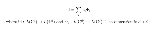
L is the space of linear operators on the d-dimensional complex vector space. How should this be understood? For example in [6] they apply a special case of this identity equation; in a run of the circuit only one of these terms (one channel) is applied at a time. This already indicates that cutting requires running the circuit multiple times in order to simulate the identity. This makes sense intuitively, since making a cut somewhere in a circuit makes it necessary to perform a measurement. As a result, some of the entanglement / quantum properties of the circuit are lost. To compensate this, one has to artifically simulate this quantum behaviour by sampling (running the circuit more often). This so-called sampling overhead can be proven to be

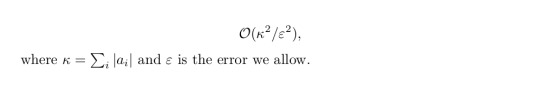
This can be derived with the help of defining an unbiased estimator and applying Hoeffding's inequality. A detailed derivation (which holds for general operators, not only for the identity) can be found in appendix E of [3]. The exact sampling cost depends on the explicit decomposition one wants to apply.

Closing remarks

Up to my knowledge, those circuit cutting schemes only work efficiently for special cases. Often, the cost depends on the size of the cut, i.e. how many wires are cut. Additionally, the original circuit should be able to be partitioned reasonably. In the title picture you can see a mock circuit with five qubits. You can see that on the left side of the cut, there are gates which act on the first three (1,2,3) qubits only, while on the right side they only act on qubits 3,4 and 5. Hence, the cut should be placed on the overlap on both parts, i.e. on the middle qubit (3). The cut size is only one in this case, but in useful applications the cut size might be much larger. Since the cost often depends on the dimension of the cut qubits, the cost increases exponentially in the cut size (since the Hilbert space dimension grows as 2^k for the number of cuts k).

Thus, we see that circuit cutting can be very powerful in special problem instances, in which it can e.g. reduce the required qubits roughly by half - this helps making circuits shallower and smaller. However, there are lots of limitation given by the set of suitable problem instances and the sampling overhead.

--- References

[1] Marvin Bechtold, Johanna Barzen, Frank Leymann, Alexander Mandl, Julian Obst, Felix Truger, Benjamin Weder. Investigating the effect of circuit cutting in QAOA for the MaxCut problem on NISQ devices. 2023. arXiv:2302.01792

[2] M. Cerezo, Andrew Arrasmith, Ryan Babbush, Simon C. Benjamin, Suguru Endo, Keisuke Fujii,��Jarrod R. McClean, Kosuke Mitarai, Xiao Yuan, Lukasz Cincio, Patrick J. Coles. Variational Quantum Algorithms. 2021. arXiv:2012.09265

[3] Christian Ufrecht, Maniraman Periyasamy, Sebastian Rietsch, Daniel D. Scherer, Axel Plinge, Christopher Mutschler. Cutting multi-control quantum gates with ZX calculus. 2023. arXiv:2302.00387

[4] Kosuke Mitarai, Keisuke Fujii. Constructing a virtual two-qubit gate by sampling single-qubit operations. 2019. arXiv:1909.07534

[5] Tianyi Peng, Aram Harrow, Maris Ozols, Xiaodi Wu. Simulating Large Quantum Circuits on a Small Quantum Computer. 2019. arXiv:1904.00102

[6] Angus Lowe, Matija Medvidović, Anthony Hayes, Lee J. O'Riordan, Thomas R. Bromley, Juan Miguel Arrazola, Nathan Killoran. Fast quantum circuit cutting with randomized measurements. 2022. arXiv:2207.14734

[mysteriousquantumphysics]

Happy Pi Day 2023!

[mysteriousquantumphysics]

ZX Calculus - Another Perspective on Quantum Circuits. Part II

Last time we introduced basic definitions and a small set of rules of the ZX calculus. While our aim is to analyze the Bell circuit in terms of this framework, you can find more sophisticated examples in [2, pp. 28]. For the Bell circuit we only need one further ingredient:

Cups and Caps

Cups and Caps are the ZX-type representations of the Bell State |Φ^+>. As you surely know, this state "lives" in a four dimensional Hilbert space, and can be represented as a vector with four entries - and in the ZX calculus this means:

In more complicated circuits it is neat to know that this Bell state actually acts as a bended piece of wire, which introduces a lot of flexibility in one's modifications of an expression. The cups and caps are merely vectorizations of the 2x2 identity matrix.

Application to the Bell Circuit

A brief reminder about the Bell circuit: It just applies a Hadamard and a CNOT on the input qubits. The outcome is supposed to be the Bell state |Φ^+>, i.e. a cup, as desribed above.

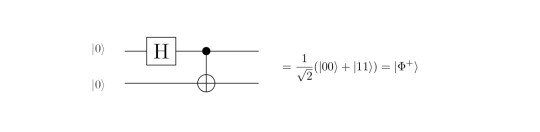
First, start by translating the circuit into ZX-language, by using the definitions we found in the previous entry. The circuit becomes:

Here, we simply expressed the |0> vectors as grey dots on the left, then applied a Hadamard on the first and afterwards a CNOT. Application of the Fusion rule on the two grey dots on the bottom yields:

Then, we apply the Hadamard on the grey dot (|0>) which changes its color:

Thus, we can again fuse two dots, in this case the two white dots above:

Then, we know that dots with a single income and outcome leg are actually just identities! As a result, our expression simplifies:

And this is exactly the cup we desired! Translating the circuit into ZX-language and applying the rules led us to the result that we have a Bell state in the end. Of course one could have evaluated this circuit easily by hand with the help of the matrix representations of the gates - nevertheless, I think it is a neat example to see the simplicity and beauty of the ZX-calculus. Check out [1] for more sophisticated examples!

Conclusion

Similar as tensor networks in general, the ZX calculus is a neat and beautiful framework which gives rise to a rich variety of applications - even though they resemble a lot, both are specifically tailored for different applications. A nice property of the ZX calculus is that it is universal: it can represent all 2^n x 2^m matrices and simultaneously it is a very intuitive and pictorial description [1, p.18]. As a final note: If you're familiar with condensed matter and tensor networks, you know that the AKLT state is of particular importance. It can also be described with the help of ZX Calculus and the framework is able to reveal its interesting properties as e.g. the string order [2].

--- References: The ZX graphics were created with tikzit.github.io. Furthermore, you can find a lot of valuable information on zxcalculus.com. [1] ZX-calculus for the working quantum computer scientist - Wetering. 2020. arXiv:2012.13966 [2] AKLT-States as ZX-Diagrams: Diagrammatic Reasoning for Quantum States - East, Wetering, Chancellor, Grushin. 2021. doi.org/10.1103/PRXQuantum.3.010302

[mysteriousquantumphysics]

I couldn’t resist to post this on Valentine’s Day, haha(:

[mysteriousquantumphysics]

ZX Calculus - Another Perspective on Quantum Circuits. Part I

Recently, stumbled across a tensor network-type framework which was completely new to me - the ZX Calculus. The ZX Calculus is not only a neat way of representing possibly complicated mathematical equations, it also gives explicit rules to alter and simplify those expressions. The ZX Calculus is particularly suited to describe matters in quantum information, which is why I'd like to provide a neat example of how to use this framework. As you might already know, quantum circuits can be fully analysed and understood with the help of tensor networks (actually, they are tensor networks) [1]. However, the ZX Calculus is a specific framework which gives a very illustrative graphical way of understanding quantum circuits, while the typical tensor network approaches are mostly tailored for many body problems. All of the following is taken from [2], a very comprehensive introduction to the ZX Calculus and I fully recommend to go through this paper if the following glimpse into the topic made you curious.

In the following we will set up the very basic set of definitions and rules in order to understand how to evaluate the outcome of the well-known Bell circuit which creates a maximally entangled Bell state:

Basic Definitions: Spiders and Vectors

The most fundamental definition in the ZX Calculus is the spider. The Z-Spider has n inputs and m outputs and is defined as follows:

Thus, such a spider is simply a way of representing a specific kind of 2^n x 2^m matrices. Here, the |0> and |1> denote the basis states of the Pauli Z operator. Similarily, an X-Spider can be defined in terms of another basis, the eigenstates of the Pauli X operator, |+> and |- >:

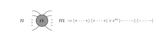
Thus, the color of the dot encodes information about the basis. The usage of the basis states of both Pauli X and Pauli Z is eponymous for the ZX Calculus. One could have chosen the Pauli Y basis as well, however the choice of X and Z results in nice symmetry properties [2, p.22]. From this, we can already conclude the first identity which we will need to evaluate the Bell circuit: Set n=m=1 as well as α=0. With these parameters, the spides become plain 2x2 identity matrices (just look at the definitions!). While α=0 is denoted with an empty dot, this observation can be represented as:

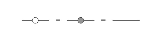
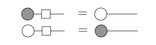
Thus, as soon as we encounter single, plain dots with one incoming and one outgoing leg, we can remove them. Additionally, we will need to know, how to represent simple basis vectors in this diagrammatic language. This is simply done by using dots with a single leg and the following simple consideration according to the definitions of the spiders:

Of course, one can also describe |- > and |1> states, just apply α=π respectively. Note that we omit global phases here; thus using a simple equality sign is actually a delicate matter.

The Hadamard Gate

The Hadamard gate is a unitary gate which simply transforms between the X and Z basis; e.g. applying the Hadamard gate to a |0> state will result in |+>. Its graphical representation is just a plain box with one outcoming and one incoming leg - its action on the basis vectors is as follows:

Actually, this is one special case of the more general rule, that the application of Hadamards changes colors as follows:

This of course also holds if the colors are inversed. In general, all ZX rules hold under coherent exchange of colors.

The CNOT Gate

Another central gate in quantum computing is the CNOT gate, which is a controlled NOT gate, i.e. the target qubit is only flipped if the control qubit is |1>, otherwise nothing happens. This 2-qubit-gate can be represented as

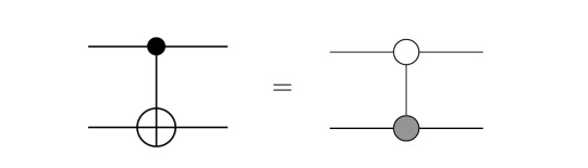
The equality sign should be taken with care as well, because the left is in the quantum circuit notation, while the right is in ZX calculus notation. Its construction is explicitly explained in [2, pp. 11]. Since it is a bit lengthy to go through it by representing the diagrams as matrices, I leave it to you to check it in the reference in case you are interested.

The Fusion Rule

In general, it is possible to "fuse" dots of the same color, while adding their phases. Note that it is addition mod 2π because α and  β are the exponents of e.

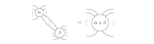
Later, we will only use a special case of this, namely that we can fuse dots of the same color which are connected by one line.

Now, we have finally settled the rough framework for analyzing the Bell circuit, which will do in the next part!

--- References: The ZX graphics were created with tikzit.github.io. Furthermore, you can find a lot of valuable information on zxcalculus.com. [1] Tensor Networks in a Nutshell - Biamonte, Bergholm. 2017. arXiv:1708.00006 [2] ZX-calculus for the working quantum computer scientist - Wetering. 2020. arXiv:2012.13966

[mysteriousquantumphysics]

Studying in China Remotely from Germany - Some Experiences

As I have mentioned in a previous entry, the past winter term I studied at Tsinghua University in Beijing. Unfortunately, I could not enter the country due to the Covid restrictions that have been still present when the semester started - nevertheless, I thought it might be valuable to share some experiences.

Studying Remotely

What had been a frustrating experience is that the exchange semester - which I had started organizing in summer 2021 - could not take place in person. The exchange semester started in September 22 and the information that exchange students cannot enter China was sent by the end of June 22. Thus, it was only roughly two months before the semester started until I knew for sure that I will not study on Tsinghua Campus. This had been unfortunate, because I was thinking about cancelling the exchange but it was too short to organize something else in Germany, as for instance an internship. I could have expected that it will not work anyway but somehow I kept some naive optimism until I knew for sure. Hence, after some considerations (Tsinghua expected a response already about one week after they sent the notice) I decided to do the exchange semester nevertheless. Even though this meant not having access to most of the experiences that make an exchange semester worthwhile and spending another semester mostly at home - even though there are nearly no Covid restrictions in Germany anymore. Back then, I was at least happy that I could avoid the risk of ending up in a harsh Chinese lockdown - the opposite happened: China gave up most of its Covid regulations. I’m happy and I hope that future exchange students will be more lucky than me in this respect.

Choice of Lectures

Since the lectures made up nearly everything of my exchange experience, it was also a little frustrating to see in the beginnning that the offered lectures in English are very limited at Tsinghua University - also regarding the point that one got access to the lecture lists only roughly a week before the semester started. In particular, nearly all useful lectures of the Physics Department were held in Chinese, which was unfortunate because I was enrolled as a student of this department and there were regulations that one was only allowed to do a very limited amount of credits outside the own department. Nevertheless, I tried to do the best out of it and attended at least one lecture (the only one which was in English and somehow useful for me) of the physics department about topological materials from an experimentalist’s standpoint. I already attended a theory course about this topic at TUM but at least I got a new perspective on some issues in this field.

Eventually, I also found interesting courses in the realm of computer science: one about theoretical informatics (automata theory) and machine learning. The latter was the most useful course in the whole semester because it covered a lot of different machine learning techniques, some of its mathematical background but it mostly focused on its application. The course offered a lot of programming exercises as well as a larger programming project which did not only help me to think through a more complex task but also gave me the opportunity to work together with Chinese students. In particular because I want to focus on numerical physics in my future and machine learning techniques become more and more prominent in physics, this computer science related lecture was very useful.

Last but not least, I also attended a course about Wittgenstein’s Tractatus, a lecture completely beyond my scientist-horizon. But it was a nice experience because it required a different kind of thinking than I am used to, even though analytical philosophy also covers aspects of philosophy of mathematics and science. I guess it is smart to learn a subject outside the bubble of quantitative science as well because it gives you some new perspectives which you usually easily ignore but shouldn’t.

Time Shift and Learning Mandarin

One further important point about studying remotely is the time shift of course. Between Munich and Beijing it is 6 or 7 hours difference (depending on the daylight saving time in Germany). Fortunately, most of the lectures were recorded anyway such that one could avoid living in another time zone. What one could not avoid was writing (midterm/final) exams in the middle of the night, what was definitely demanding.

Regarding learning Mandarin: I started learning Chinese one year before the exchange semester started, but to be honest I doubt it would have been enough for basic communcation in the supermarket. Even though Chinese has rather easy grammar, learning to understand the tones and the ambiguities in this language is the true challenge. However, it would have been truly useful to have more Mandarin skills: The online portals of the university are in Chinese of course and often I experienced that I could not access everything with the English counterparts. Another important point is that not all lecturers take English as instruction language so seriously: In one lecture many exercise materials had been in Chinese (and the topic was too technical to translate with baidu) such that exchange students had a clear disadvantage - but I want to emphasize that this depends on the lecturer - most of my lectures had been organized perfectly in English.

Conclusion and Hints

All in all, I hope I was able to make the best out of this exchange semester. I have mostly chosen lectures which were beyond my known horizon but nevertheless not useless in my discipline. Nevertheless, I could have attended lectures at my home universities which would have been much more favorable from an academic perspective. However, I think it was also nice to be forced to study outside the own discipline and to learn subjects I would have never decided to learn at TUM and LMU. Nonetheless, I still find it surprising that an elite university as Tsinghua offers most of its lectures in Chinese - in particular TUM and LMU are contrasting starkly regarding this, because here all lectures (at least at the physics departments) are held in English at the Masters level. 

Hence, I think this online exchange semester was a worthwhile experience despite all these issues. Finally, I am also happy that it is over and that I will start my Masters thesis soon here in Germany. I’m glad to have the chance to dive completely into (numerical) physics and related research questions! 

Finally, some hints if you’re planning to do an exchange semester in China (from my limited perspective as I haven’t been there in person)

When planning the exchange also develop a plan B: For me it would have made things so much easier if I had planned something in parallel (e.g. an internship in Germany) because then my decision of doing the exchange semester or not would not have been based on the lack of good alternatives.

Be patient: The administration (at least as I experienced it at Tsinghua) is rather slow and it happened that I never received answers to my e-mails. 

Be open-minded: As I explained in detail, lectures are mostly held in Chinese and one has to be flexible with the course choice in English. If you stick to the idea of remaining in your own discipline, an exchange semester will be a frustrating experience.

[mysteriousquantumphysics]

Data Science meets the Many Body Problem

Since the machine learning course I did this semester at Tsinghua university was mainly focused on typical data science applications, I was curious in how far those methods can be applied in physics. Of course it is nothing new that neural networks can in principle also be used for physical applications - however, tensor network methods still seem to be dominant in the field of numerical many body physics. Thus, I decided to dive in a little into the literature about the usage of Restrictive Boltzmann Machines (RBM) in many body physics.

What are RBMs?

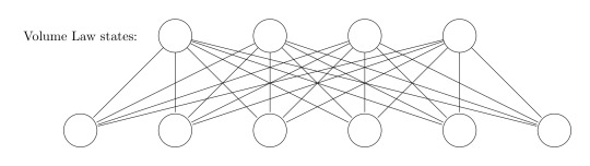
Usually, RBMs are used for instance for recommendation tasks (e.g. video recommendations on video platforms) and many more. In general, it is a unsupervised learning technique which makes use of minimizing its "energy". Thus, the intuition behind RBMs is, despite their data science applications, already related to physics: We will see that it is no surprise that "Boltzmann" is part of the name of this method. An RBM utilizes input data, tries to extract meaningful features from it and wants to find the probability distribution over the input. This follows the physical intuition as follows: The RBM is a neural network with two layers, a hidden and a visible layer, where each node can adopt binary values. An example network looks like:

where the x denote the visible nodes, the h the hidden nodes and W denotes the weights between both layers. Note that there are no links in between the nodes of a single layer; this is why these networks are called restricted Boltzmann machines.

The network is governed by a corresponding energy function as:

where we also have the offsets of the single nodes (a for the visible nodes and b for the hidden nodes). Given this energy function, one can determine the probability distribution by the Boltzmann distribution where Z is a partition function, as familiar from classical statistical physics. As usual, the energy is supposed to be minimized, what is done by the learning algorithm of the RBM but this should not explained here since it would go beyond the scope of a brief blog entry. At this point I'd only like to mention that there are some difficulties determining e.g. the partition function (which is intractable in general) and that this requires some sophisticated algortihms. If you're interested in this and how the RBMs work exactly, a neat and far more rigorous introduction into RBMs can be found here.

One side note at this point: RBMs were introduced by Geoffrey Hinton after John Hopfield (a physicist) invented the so-called Hopfield networks which are also such an energy based mechanism, based on the physical intuition of Ising models.

Note that so far we only talked about the RBMs as they are used in data science - despite their physical intuition, they had so far nothing to do with neither quantum mechanics nor the many body problem. This is what comes next.

How can this be linked to condensed matter?

As introduced in [1], an RBM that can represent a quantum many body state would look like this:

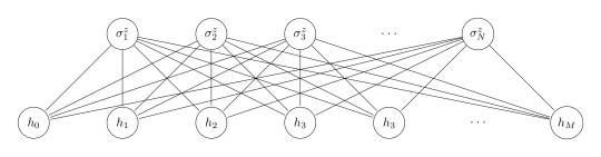
In comparison to the previous network we changed the labels from x to σ, where the σ's denote e.g. spin 1/2 configurations, bosonic occupation numbers and so on. For them one has to choose a basis, e.g. the σ^z basis. This configuration can be summarized in the set S. Hence, the visible nodes are the N physical nodes of the system. The M hidden nodes h play the role of auxiliary (spin) variables. The authors describe the understanding of such a neural-network quantum state as follows: "The many-body wave function is a mapping of the N−dimensional set S to (exponentially many) complex numbers which fully specify the amplitude and the phase of the quantum state. The point of view we take here is to interpret the wave function as a computational black box which, given an input manybody configuration S, returns a phase and an amplitude according to Ψ(S)" [1, p.2]. Thus, one gives a certain spin configuration as input and the RBM generates the state, in the following form:

Thus, once can recognize that the form of such a neural-network quantum state adopts a similar form as the aforementioned Boltzmann distribution (exponential of energy function). However, there is additionally a sum over all possible hidden configurations which specifies the full state. After setting a state up in this form, one aim could be to find the ground state corresponding to a certain Hamiltonian, and according to the authors of [1], their RBM method gives decent results for this task!

Similarity to tensor networks

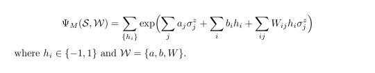
Interesting is, that this framework (even though it appears very different) has some analogous quantities as tensor network states. For example, the representational quality of a neural-network quantum state can be increased by increasing the number of hidden states: Thus, the ratio M/N plays a similar role as the bond dimension of a tensor product state! There are many more similarities, which should not be discussed here but can be found in [3].

Nevertheless, I'd like to mention an important distinction, which is also crucial for tensor network states, because some algorithms (DMRG etc.) can only handle area law states properly. While volume law states have an entanglement entropy which scales with the volume of the partitions of a state, an area law state has a scaling only proportionally with the area of the cut. Area law states can be handled better numerically, because the bond dimension of tensor network states explode for volume law states (more on tensor networks and area law can be found in [4]). According to [2] the difference between area law states and volume law states can be captured in a neat way with RBM states: While volume law states must have full connections between the hidden and physical nodes, an area law state has fewer links - this imposes locality in a sense. The RBM states thus give a neat intuition between the differenece of both kinds of states.

All in all, RBMs seem to be an interesting approach to connect both data science methods and many body physics. It may be that they have strengths which the usual tensor networks approaches lack: for instance, the authors of [2, p.888] claim that it might be possible that RBMs might be able to handle volume law states better than usual tensor network approaches do, which would be of course a major benefit. Since I haven't heard of this approach within the condensed matter framework before, I'm very curious how the importance of this method will evolve in future research!

--- References:

[1] Carleo, Troyer, Solving the Quantum Many-Body Problem with Artificial Neural Networks, arXiv:1606.02318

[2] Melco, Carleo, Carrasquilla, Cirac, Restricted Boltzmann machines in quantum physics, https://doi.org/10.1038/s41567-019-0545-1

[3] Chen, Cheng, Xie, Wang, Xiang, Equivalence of restricted Boltzmann machines and tensor network states, arXiv:1701.04831

[4] Hauschild, Pollmann, Efficient numerical simulations with Tensor Networks: Tensor Network Python (TeNPy), arXiv:1805.00055

[mysteriousquantumphysics]

Hi, sorry for being so inactive currently! This winter term I'm pursuing an online exchange at Tsinghua University and since my subjects there are rather related to computer science than to physics it has been difficult so far to find sufficient time to dive into nice physics topics suitable for this blog! But I hope I'll be more active again soon!:)

[mysteriousquantumphysics]

Darwinian Evolution as thermodynamics in disguise?

As you know, biology is definitely not my area of expertise, but I recently stumbled accross some papers which catched my interest. Even though biology is supposed to have laws acting on a completely different "layer of complexity" than physics, some authors ([1, 2, 3] and the references therein) suggest that it might be possible to formalize at least evolutionary processes in a similar manner as thermodynamics. In the following I note some aspects of these papers which make this idea intriguing, but I wholeheartedly suggest that you check out the references themselves!

As thermodynamics is only applicable in the so-called thermodynamic limit, this holds also true in the suggested thermodynamic description of evolution [2]: i.e. it requires a large number of particles/organisms to make the thermodynamic description valid. As in thermodynamics, regarding solely small numbers of particles makes the description problematic since fluctuations and random processes cannot be neglected, the same holds for populations which are too small - the behaviour of populations can only be described faithfully on a large enough scale.

Two Opposing Principles: Maximum Entropy and Learning

As it is well-known, the principle of maximum entropy is of major importance in physics. It states that the probability distribution of an ensemble must be such that the entropy is maximized under appropriate constraints. This means that one chooses the configuration of a system which is compatible with the prior knowledge about itself and maximizes the entropy. This becomes intuitive if one regards a gas of some kind of molecules in a box: The configuration of the system is most likely to be an equal distribution of molecules thoughout the box (high entropy) while having all molecules in one half of the box (lower entropy) will not happen in reality. However, organisms work differently. They do not only increase the entropy but also decrease it, i.e. they organize/learn: The authors [2] suggest that it is required to formulate an opposing principle, the "second law of learning", where learning can be formalized in the sense of neural networks [3]. The important point is that the learning-law decreases the entropy (increases the "order" of the system) while the endeavour of the principle of maximum entropy is to increase the entropy - hence, evolutionary processes might be described by an interplay of these two opposing principles.

By defining an appropriate loss function (within the neural networks picture) one can maximize the entropy via Lagrange multipliers and derive a partition function Z, which is central in thermodynamics (for details of the derivation etc. please check [2] p. 2-3). If you took a thermodynamics/statistical mechanics course before, you know that once the partition function is known, one can derive a lot of other useful quantities, such as the free energy F. In the proposed picture of using thermodynamics to describe evolutionary processes, the partition function also has a definite interpretation: "Z represents macroscopic fitness or the sum over all possible fitness values for a given organism, that is, over all genome sequences that are compatible with survival in a given environment, whereas F represents the adaptation potential of the organism." [p.3, 2]. For me, it is pretty intruiging that it seems to be possible to reformulate such familiar notions from thermodynamics for the use of describing evolutionary processes.

Major Transitions in Evolution as Phase Transition

Moreover, the authors describe that so-called major transitions in evolution (such as the formation of cells out of pre-cellular life, origin of eucaryotes, etc.) can be described as phase transitions. We've been talking about phase transitions before as well as their major relevance in e.g. condensed matter physics - hence, it is intruiging and surprising to apply this concept to evolutionary processes. It is possible to define a quantity called "evolutionary temperature" which can be tuned, and at a certain critical "evolutionary temperature" the phase transition takes place. The phase transition is considered to be of first-order, and the authors note: "To describe phase transitions, we have to consider the system moving from one learning equilibrium (that is, a saddle point on the free energy landscape) to another." [p. 4, 2]

The proposal is phenomenological, not fundamental

As closing remarks, it should be noted that also lifeless matter can exhibit some features of life, e.g. crystals grow and some behaviour of glasses can be very roughly brought in relation to some phenomena of living organisms [p.4, 1].

Despite of all this fascinating formalism, it is important to note that these formulas will not be an explanation of evolution on a fundamental level. Of course, life is a far more rich phenomenon which can impossibly be explained by the straight forward formulas of thermodynamics. Also Katsnelson, Wolf and Koonin note that "Biological entities and their evolution do not simply follow the ‘more is different’ principle but, in some respects, appear to be qualitatively different from nonbiological phenomena, indicative of distinct forms of emergence that require new physical theory." [1] However, it is important to be aware that the aformentioned approach does not even claim to be a fundamental explanation - instead, it is a phenomenological way of describing the observed phenomena. Exactly as thermodynamics within the realm of physics is no fundamental theory, it is phenomenological and yet it has the power to explain a very wide range of phenomena.

---

Bibliography

[1] "Towards physical principles of biological evolution", Katsnelson, Wolf, Koonin, 2018

[2] Thermodynamics of evolution and the origin of life, Vanchurin, Wolf, Koonin, Katsnelson, 2022

[3] Toward a theory of evolution as multilevel learning, Vanchurin, Wolf, Katsnelson, Koonin, 2022

[mysteriousquantumphysics]

Slowly finishing my preparations for my last exam this summer term...

[mysteriousquantumphysics]

How iMPS Can Shed Light on the Distinction between Symmetry Protected Topological Phases. Part II

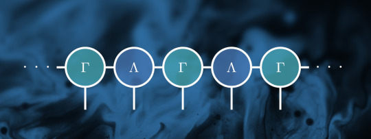
Previously we introduced some notions from representation theory and how infinite chains can be usefully represented via infinite matrix product states (iMPS). Now, the actually exciting part comes: We connect both parts, symmetries and iMPS. First, we start by checking how symmetries, i.e. their (projective) representations act on an iMPS.

Symmetries in iMPS

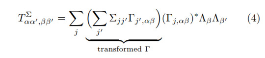
Given a system which is invariant under a certain internal symmetry with matrix representation Σ, the corresponding transformation of the Γ tensors must leave the whole iMPS invariant. This action works as

at a single Γ tensor. The diagrammatic representation looks as follows:

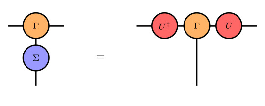
One can see that there is only a single contracted leg on the left hand side which is the reason why we only sum over j' in Equ. (3).

The elements of the symmetry group are denoted by g (which are omitted in the diagrammatic representation). Hence, by acting on one site with the symmetry representation, one gets a set of phases e^(i θ_g) and one of unitary matrices U_g if one regards all elements g of the symmetry group. The phases form a 1D representation (character) of the symmetry group, while the U_g form a projective representation, i.e. their homomorphism property is expanded by a phase, as we introduced in the previous entry. The resulting factor set can distinguish between different symmetry protected topological phases of the system. How can one practically retrieve the U matrices? By applying iTEBD or iDMRG one can retrieve the ground state of a given system, which will be provided as an iMPS in canonical form. Then, one knows that transforming a state by the symmetry should leave it invariant. Thus, the overlap between the original and transformed state has to remain <ψ|ψ'>=1. This inner product consists of several ``generalized'' transfer matrices:

Due to the required normalization, the largest eigenvalue of this generalized transfer matrix must be η=1, otherwise the state is not invariant under the given symmetry. We denote the corresponding eigenvector X_αα' (which is actually a matrix but can be shaped into a vector by vectorization). This gives us the anticipated U matrix, which is related to the eigenvector as

which can be explained by how the symmetry representation Σ acts on the Γ tensors as described in Equ. (3). Due to the fact that the U are unitary, only one U^† will effectively remain in the expression. This sole U^† can then be related to the eigenvector X from the fact that the iMPS is in canonical form. A diagrammatic representation of this computation works as follows:

First, we have a fraction of the generalized transfer matrix (Equ. (4)). Afterwards, we apply Equ. (3) and this yields:

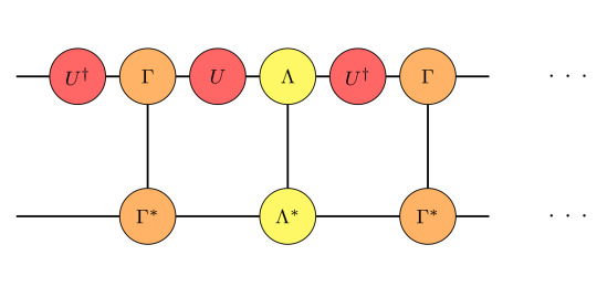
From the fact that the U are unitary and commute with Λ, one can simplify the expression as:

The remaining U^† can be related to the left eigenvector of the transfermatrix via Equ. (5). How this helps us to numerically distinguish the phases will be regarded in the next section, where we regard a specific example.

Application to the Spin-1 Chain

Let us consider a spin-1 system evolving under the Hamiltonian

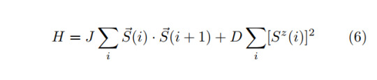
which gives rise to a symmetry protected topological phase. Note that the first term describes the usual Heisenberg model, while the second is an anisotropy of the system. Even though one can study more symmetries of this system, let us focus on the Z_2 x Z_2 symmetry. The representations Σ are given as

Previously, we mentioned that the factor set of a projective representation can be linked to a distinction of topological phases. In the present case this works as follows. Note that the Z_2 x Z_2 symmetry is abelian, i.e. the group elements commute. For a general projective representation U with group elements g and h, this means:

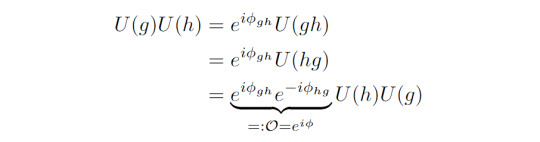
where we used the homomorphism property of the projective representation twice.

Applying this to the present Hamiltonian one will end up with two different values of the curly O which can distinguish the phases:

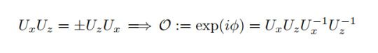
Here, ϕ can either be 0 or π, leading to O=+1,-1.

Having said this, the practical, numerical method to find the phases according to the Z_2 x Z_2 symmetry in the present system is the following: First, one implements the Hamiltonian such that it suits iTEBD. Then, one finds the corresponding ground state and applies the symmetry matrices R_x and R_y in order to retrieve the overlap in the form of the generalized transfer matrices. Afterwards, one takes one of the transfer matrices and diagonalizes it (via sparse matrix methods, e.g. Lanczos). Having implemented this, one can check for which parameters of D and J the largest eigenvalue is indeed 1 (if it is smaller than 1, the symmetry is not conserved in this phase, i.e. O=0). After this step, one can find the U_x and U_y by Equ. (5) and one can determine the phase as described above and find two distinct phases preserving the symmetry: a trivial, O=+1, and a topological, so-called Haldane phase, O=-1.

Now, the overall result we achieved is that we found values which are capable of characterizing a topological phase. This is important, since topological phases do not obey the Landau paradigm and can therefore not be distinguished by spontaneous symmetry breaking. Hence, it is remarkable that one can find a way to distinguish these new phases by combining representation theory and MPS methods. There are even more methods to distinguish the symmetry protected phases in such 1D chains - in case you're interested, have a look on the remainder of [1].

---

References

[1] Pollmann, Turner. Detection of symmetry-protected topological phases in one dimension. Phys. Rev. B 86, 125441. 2012.