#studblr
Text

Heading into the new year, it’s important to take a moment to be grateful for what you have, and where you’re at as you set goals for 2023.
Don’t forget the present while pining for the future 🤍
Art by @madebynelson on IG and Twitter
#gratitude#slow living#aesthetic#grad student#gradblr#studblr#pause#yoga#mindfulness#mindfulthinking#minimalist#new year
2K notes
·
View notes
Text
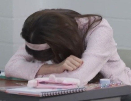
dead emotionally, but keep studying as hell


294 notes
·
View notes
Text

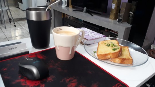
My coffee 🤎☕️
قهوة بسيطة 🤎🤎
By me @un-known97
#마드#mobilephotography#art#photography#myshots#mycam#mine#coffee#coffetime#coffeetime#cup of coffee#my coffee#coffeeblr#coffeelover#morning coffee#mood#studblr#tumblr#Artist#tumblr staff#photographers on tumblr#artist on tumblr
90 notes
·
View notes
Text
Is there anything I can do to feel better and actually rested without feeling guilty for not doing something productive
#new rtgame video is out mb it will help#idk I just want to stop feeling like shit#ohnotalking#student life#studblr
29 notes
·
View notes
Text
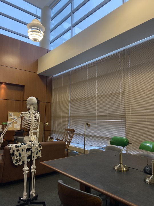
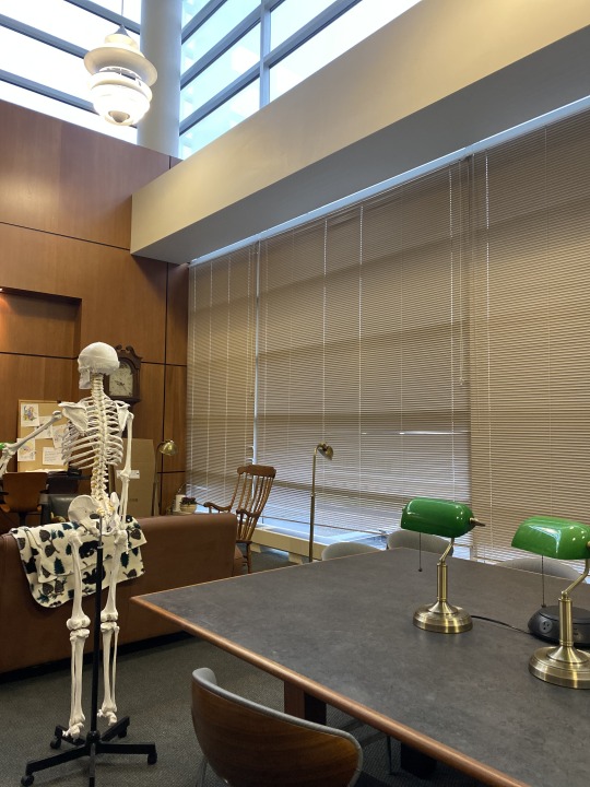
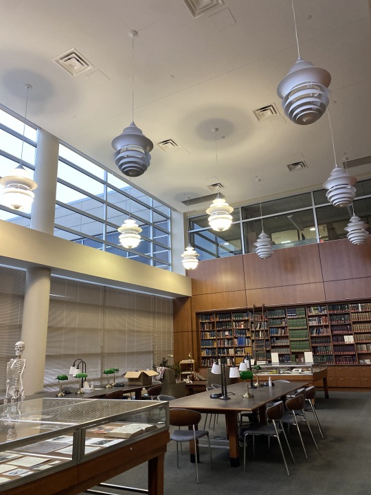
Day 5/100 of productivity
#studyblr#med school#medicine#studyspo#study motivation#aesthetic#college#anatomy#books & libraries#travel#studblr#collegeblr
25 notes
·
View notes
Text
School has been taking so much time away from what I actually want to study and pursue as a career ..
#tumblr 2014#coquette aesthetic#coquette#gloomy coquette#coquette angel#coquette dollete#dollette#nymph3t#angelic#angel aesthetic#angelcore#pink#pink core#hyper feminine#nympette#nymphetfashion#melanie martinez#crybaby#lizzy grant#lana del rey#lana del ray aka lizzy grant#preppy#studytok#studblr#study motivation#academia#light academia#sanrio#sanrio aesthetic#sanriocore
20 notes
·
View notes
Text

#academia aesthetic#light acamedia#soft academia#dark academia#text#advice#luck#books#greatness#paul graham#quote#academia#study#studblr#research#degree
15 notes
·
View notes
Text
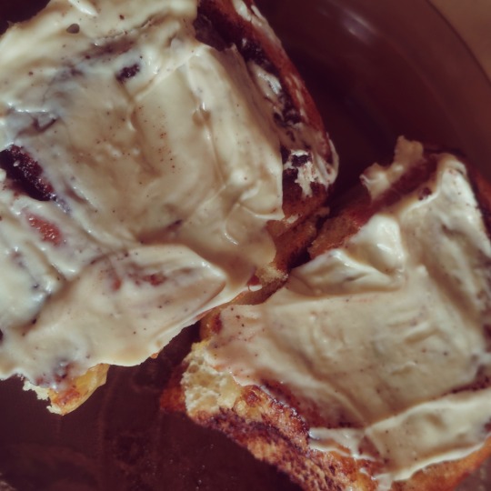


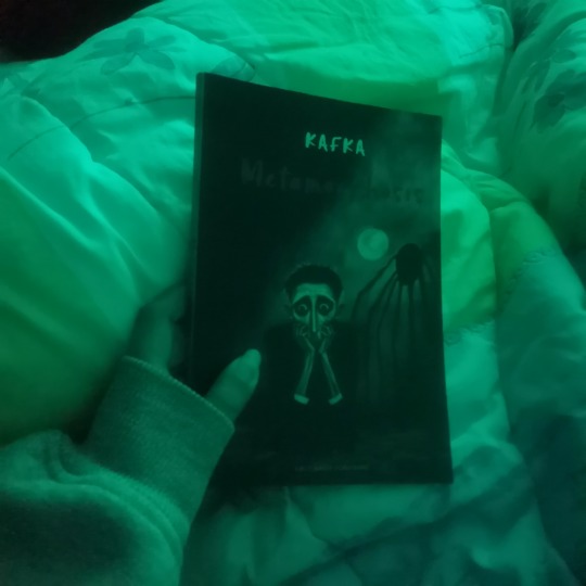
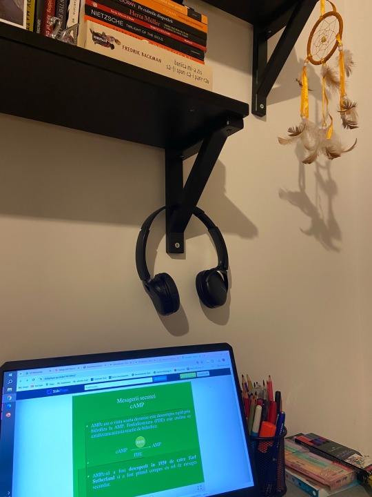
Feb 21 2024. Wednesday
Woke at 5 am to attend 2 lectures
Finished the secret history
Read a chapter of the Bible
Helped my brother with his homework
Listened to 2 Latin texts lecture records and retook/ corrected some notes
duoling streak ofc
Copied an Italian lecture notes and 2 philology lectures
In case you're wondering the 1st pics is Cinnabons covered in white chocolate but the Pic is inverted, I'm too tired to fix it tbh it's past 4 am now :') Rip me. I drank 3 cups of coffee. Can't wait to start Metamorphosis by Kafka soon, tho the cover is scaring me a bit lol! Anyways I'm dying so I'll sleep or try to?!
Have a good day/night and stay hydrated.. Also relax your muscles and jaw and take a second to breathe 😊
#student#real life#university student#uni student#student's life#university#life#studying#student life#study#classical academia#Classical studies student#Academia#Classical studies#chaotic academia#Lectures#studblr#Books#Kafka#donna tartt#the secret history#tsh#metamorphosis#Too tired#Sleepy#Txt#A day in the life#Reading#Productive
9 notes
·
View notes
Text


11 notes
·
View notes
Text

There is only a few pages left to fill until I can start a new journal!
#take time#art journal#mine#moodboard#scrapbook#journaling#studblr#space#mnemonics#math#psychology#neuroscience#conciousness#hmu if u wannna share your knoweledge on these topics#im always looking to learn new things#let me know what you are learning/ reading/ making#or if you have sideblogs on these topics
75 notes
·
View notes
Text
burnout is so real.
#study girl#girl blogging#girlblogging#academia aesthetic#study blog#studblr#study aesthetic#burnout#ughhhhhghhh
10 notes
·
View notes
Text
Quantum Circuit Cutting - with Randomly Applied Channels

Recently, I briefly introduced what circuit cutting is, why it is an advisable thing to do with current quantum hardware (NISQ devices) and what additional costs the cutting is causing. However, I did not go into detail how such a circuit cutting method can look like in detail - this is what this entry will be about. In particular, we will have a look on the circuit cutting procedure proposed by Lowe et. al. [1] in which randomly applied channels are able to cut a circuit.
Identity on Cut Circuits
As mentioned in the previous entry, circuit cutting requires to find a proper identity channel on the cut wires which has reasonably low sampling overhead - the definition of the identity is thus the heart of every circuit cutting procedure. In general, such an identity has the form

where Φ_i is some properly chosen quantum channel. The corresponding cost depends on the value κ

which is the L1 norm of the real coefficients of the identity channel above:

Thus, we see that the main possibility to reduce the sampling overhead is to reduce this value. One possibility with small sampling overhead is the following (however, it is not minimal! The method described in [2] has a lower overhead, but we will not go into detail of this).
The identity channel used in [1] looks like

Here, d=2^k is the dimension of the subspace governing the qubits of the cut. The variable z denotes a Bernoulli random value where z=1 appears with probability d/(2d+1). Later, we will derive this form of the identity channel and will see how this probability and also the expectation E_z emerges. Since, there are two values of z, there are also two quantum channels which can be applied. The first one, Ψ_0, is a measure-and-prepare channel:

The unitaries which are applied on the state prior to measurement have to comprise a 2-design (at least) because otherwise the derivation would not work. Such a design is formed by e.g. Clifford gates but there are many possibilities, one could also rely on approximate designs. Since the form of a quantum channel is not so pictorially, you can see in the following how this channel looks like in "circuit-language":
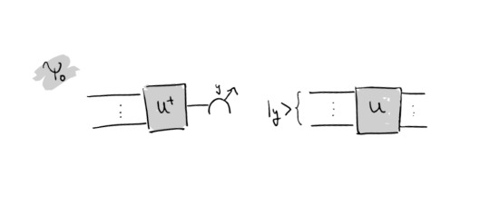
This means, one applies U^\dagger on the k cut wires, measures in z-basis and retrieves a bitstring y. A state in computational basis corresponding to this bitstring gets initialized and then U is applied. All of this is repeated many times.
Note that applying such a circuit in the middle of a larger circuit destroys entanglement of the global state and this is also the reason why cutting requires a lot of sampling (quantified by the sampling overhead): The effects of entanglement in the final result must be regained somehow by repeating the procedure numerous times.
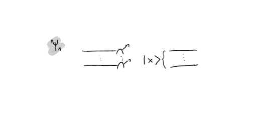
The other channel, Ψ_1, is a simpler one. It is the so-called fully depolarizing channel in which all of the information within the cut (within a sample) is lost:

In practice, the action on the cut part of the circuit is as follows: First one measures the k cut wires in the computational basis. Afterwards one takes a uniformly sampled bitstring x and initializes it on the wires - as in the following circuit snippet:
Guiding through the Derivation
Now, as we have settled the definitions, let's go through the derivation of this identity channel! At first, we need an equation which we shall not prove as this would be more involved (based on Haar measure etc.). It is called Werner Twirling Channel:

This equation is particularly nice because the right hand side is much much simpler than the left hand side, which requires all of the unitaries in the design. At the same time, the right hand side could be quickly written out by hand for e.g. d=1. This will come in handy in deriving the identity channel.
The idea of the proof is to start with one channel Ψ_0 and massage it a little to find an expression of Ψ_1 within it and then massaging it a little further and finding an expression for the identity channel.
Hence, start with the channel Ψ_0:

A lot is going on here, thus let's go through the equalities step by step: From the first to the second line the only thing happening is that we insert an identity (using completeness of the computational basis). Going to the next line, the two scalar factors are swapped and the states with index i can be used to rewrite the expression into a Tr. By exploiting the properties of tensor products and the trace, one can draw outside the sum a partial trace expression in the last line. This shape is nice, because we can recognize the left hand side of the above equation and can simplify the underbraced expression:
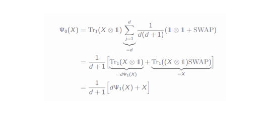
Since the expression within the sum does not depend on the index j anymore, this sum merely gives a factor d. In the second line we draw the partial trace factor into the brackets and recognize the Ψ_1 channel! Additionally, the part with the SWAP operator can be simplified as well (you can easily prove this by checking it with a 4x4 SWAP matrix and using a general matrix X). All of this helped us immensely in relating both channels to each other. Reshaping this equation a little gives us:
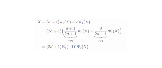
In the second line, we draw a factor outside in order to retrieve the Bernoulli probabilities we have defined previously and then, by respecting the additional sign, this can be easily rewritten as an expectation value in the last line.
What about the cost?
Now as we have both defined and derived the identity circuit expression, let's relate it to the introducing sentences about the sampling overhead. The value of κ can be easily computed:
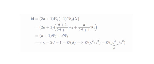
As we can see, the sampling overhead is exponential in the number of cut qubits - this is a deficit in practice. Even though, there are slightly better circuit cutting procedures, the overhead always scales exponentially in the number of cut qubits. Although unfortunate, this makes perfect sense intuitively: The cutting destroys part of the quantum properties of the system and these must be reproduced classically (by sampling). Mostly everything quantum which is simulated classically scales exponentially (since the Hilbert space dimension grows exponentially with growing number of particles).
Overall, circuit cutting is an interesting new field in quantum computing which might help to go beyond the capabilities of current NISQ devices - nevertheless, there is always a price to pay and it will become evident in future research whether circuit cutting will be a common method or not.
---
References:
[1] Angus Lowe, Matija Medvidović, Anthony Hayes, Lee J. O'Riordan, Thomas R. Bromley, Juan Miguel Arrazola, Nathan Killoran. Fast quantum circuit cutting with randomized measurements. 2022. arXiv:2207.14734
[2] Hiroyuki Harada, Kaito Wada, Naoki Yamamoto. Optimal parallel wire cutting without ancilla qubits. arXiv:2303.07340
#physics#mysteriousquantumphysics#studblr#physicsblr#quantum computing#quantum#quantum physics#quantum information#women in science#stem#stemblr
32 notes
·
View notes
Text
Some useful YouTube channels for studying coding, statistics and math

166 notes
·
View notes
Text
moodboard ♡

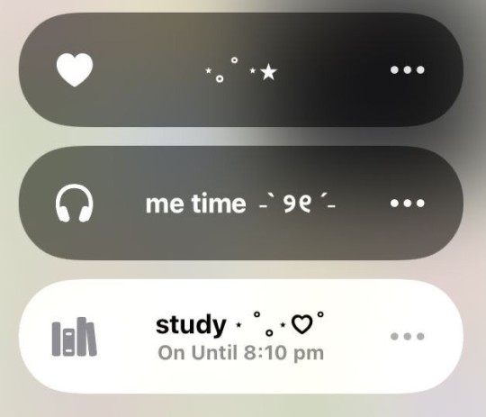
#study aesthetic#moodboard#study mood#studblr#perfect#perfect grades#student#study tips#study#studying#study motivation#study hard#study notes#study blog#studywithme#pinterest#stay focused#success#mindset#straight a student#a+#intelligent#metime#dontgiveup
34 notes
·
View notes
Text
That's it I've finished my homework so now I'm going to crawl to my bed to play my little games like I'm a person with no anxiety or responsibilities or the doom of unemployment
6 notes
·
View notes
Text

11 January - 100 Days of Productivity - 10/100
One thing I have learned working in a big company is that you will be hired for one thing, but, at the end of the day, you will have to deal with others.
I have to study Java, but also need to learn Javascript, HTML, CSS, SQL, and a bunch of other things to be able to do whatever your team needs. I will have to study forever indeed 🤔🤪
#study#studyblr#study blog#daily life#dailymotivation#study motivation#study space#studying#productivity#study desk#100 dop#100 days of coding#100 days of code#programmer#coding#studblr#I am tired and it is only January
41 notes
·
View notes
Last Seen Blogs

the5ofspades
spades

s-e-r-a-phim
SERAPHIM


freeiptvm3u
Sans titre

glasstablesonline1
Glass Table Online