#Weibull parameters | Explore Tumblr posts and blogs

juniperpublishersoceanography · 4 years ago

Text

Assessment of Centurial Extreme Coastal Climate of Bethioua Algeria- Juniper Publishers

Abstract

Nearshore marine climate at the Port of Bethioua, located on the west of Algeria, were studied using real-time field data and climatological offshore data obtained from the UK Met Office. Total waves, swells in the offshore are hind-casted separately and were validated using buoy measurements were supplied by UKMO at a nominal cost. Shallow water wave transformations are modelled using the Teluray wave-current model to calculate shoaling, depth refraction and current refraction taking bathymetry and tidal flows from the TELEMAC flow model as inputs. The results are of particular importance in the context of planning of port and safe anchorage and movement and anchoring of vessels in the harbour area, in addition, for future developmental programs at the port of Bethioua.

Introduction

Waves are of varied forms, frequencies and directions. To arrive at their climatological picture has always been a challenge to harbour engineers from strategic, economic and commercial points of view. The knowledge of sea state is essential in all operational activities in the marine environment, for the safety of public and for design of coastal and marine engineering structures. Efficacy and life of both floating and fixed marine structures and their cost analysis require good estimates of the extreme sea states [1]. Careful assessment of the wind and wave climates, employing good data and reliable analysis techniques, is necessary for the design of all modern deep and coastal ocean infrastructure systems [2]. Height and period of waves are the most important parameters required in ocean engineering designs [3].

In connection with the future developmental programs at the port of Bethioua, studies were carried out on the offshore wind and wave conditions and nearshore wave transformations in the sea off Bethioua to assess the navigation and berth operability perspectives. This paper presents the results of investigations on the winds and temporal and spatial distribution of waves in the nearshore waters of Bethioua, Algeria for 100 years. Wave activity in the port and its environs is of particular importance in the context of design of port, its operation, ship navigation, safe mooring of vessels and transport of cargo in the harbour area.

Materials and Methods

Algeria is in the Maghreb region of North Africa on the Mediterranean coast. The port of Bethioua is located on the west of Algeria. It has a gas terminal, petrochemical facilities and a desalination plant. Figure 1 gives the location of the port of Bethioua. Long term Offshore data were obtained from UK Met Office was used for the coastal process and nearshore wave data analysis. UKMO provides Wave data from operational wave forecasting model re-run in a hindcast mode with calibration against measured data from weather ships and satellites. The model results were also validated using the real-time wave rider buoys measurements. Different components of the wave energy spectrum, for example wind-sea and swell, can propagate naturally and separately, each responding realistically to changes in the wind fields. The full wave directional spectrum, which automatically includes both wind-sea and swell, can be re-constituted as required at each time step and at each grid point. Time series data were collected from offshore observation point located at 36.0 °N, 0.46 °W for twenty-year period from March 1987 to Feb 2006. Three-hourly data on wind speed and direction, significant wave height, mean wave period and mean wave direction are analysed. Data on swells generated by remote storms have been analysed separately as long period swell waves are of particular importance in the movement of moored ships. A similar attempt has earlier been successfully carried out around the Korean peninsula [4] and for the northeast Atlantic European coast [5].

The Met Office (UKMO) Global and European Wave Models represent the ocean surface's elevation due to wind stress as an energy spectrum which parameterizes the non-linear interactions in the wave spectrum. The behavior of the individual spectral components (i.e. their growth and dissipation) can be computed. In each 30 minute time step, the wave energy components move in their respective directions through the a directional spectrum which has 16 and direction (θ m) at each grid point can be integrated out from direction and 13 frequency grid. The significant wave height (Hs), mean wave period (Tm) components.

Shallow water transformations of waves consist of refraction, depth induced breaking and shoaling. Shoaling involves changes in wave height due to the waves slowing down as they travel through water of decreasing depth. Refraction involves gradual change in wave direction as waves travel towards the coast, with the wave crests tending to align more nearly parallel with the seabed contours [6]. Added to these are the influences of tidal currents causing changes in wave height. The current effects on waves are likely to be important where peak tidal velocities exceed about 2m/s [7]. In regions where there are strong tidal currents, the influence of tidal currents on waves (current refraction) is just as important as depth refraction and shoaling. An accurate prediction of the combined effects of depth refraction and current refraction is important in engineering studies in harbours.

Generally, in wave transformation studies selected offshore wave conditions from the probability estimates will be transformed using standard numerical models to study the nearshore wave parameter, which gives biased results. Ultimately, it may cause overestimation/underestimation, hence it increase the error in planning and cost estimation.

The present study makes use of the Teluray wave-current model to calculate shoaling, depth refraction and current refraction taking bathymetry and tidal flows from the validated TELEMAC2D flow model as inputs. The Teluray model predicts nearshore wave activity by representing the effects of refraction and shoaling on all components of the offshore spectrum using a backtracking ray method. It employs an unstructured finite- element model mesh, which allows the dynamic variation of resolution, so that better resolution can be achieved in areas of particular importance. Figure 2 shows the model mesh for Bethioua.

By this approach, we are transforming each offshore wave ray to the corresponding wave at a neashore point of interest with the influence of all corresponding possible natural agents like wind, tidal variation and processes like shoaling, diffraction etc. Sensitivity tests were conducted to test the model sensitivity to different parameters in the numerical model and were calibrated with available in-situ measurements. Result of the study is a nearshore time series to the corresponding offshore time series at a point of interest. The resultant nearshore time series will be further utilised in estimation of wave parameters for next 100 years using a Weibull fit.

Results and Discussion

Offshore winds

Spatial and seasonal variations in wind and wave conditions are of particular interest when considering safety and ease of manoeuvring and mooring of vessels in the harbour area.

(Data in parts per hundred thousand; U is the hourly averaged wind speed in m/s; P(U>U1) is the probability of U10 exceeding U1).

(Total number of hours in period = 166560).

Wind conditions offshore of Bethioua are presented in Figure 3 as a rose diagram. The area is mostly influenced by westerly and northeasterly winds. Winds blowing from the sector centred at 270 °N are the strongest having speeds in the range 24-26m/ s. The most frequently occurring winds are from 240 °N, which account for 18% of records. Table 1 gives the annual average wind climate offshore of Bethioua. Table 2 presents the average monthly probability of exceedence of wind speeds offshore of Bethioua for all the months based on wind data for March 1987 - February 2006. The wind climate of the region consists of two seasons. The winds are strongest during winter months (October-April) and relatively calm during summer months (June-September). Figure 4 presents the diurnal variation of average mean wind speed for all months at the observation point located at 36.0 °N, 0.46 °W. The wind speed shows higher variations during summer with average mean speed reaching a maximum in the afternoon (15:00 GMT) with slower wind in the early morning (06:00 GMT). The greatest variation in mean speed is seen in August with mean speeds ranging between 4.0m/s and 6.0m/s. Diurnal variations are much lower in mean offshore wind speed during winter months.

Offshore waves

The offshore wave climate is presented in Tables 3-5 as scatter tables of significant wave height (Hs) in metres against mean wave direction, significant wave height against mean wave period (Tm) and significant wave height against hourly averaged mean wind speed (U) in m/s respectively. The data, in parts per hundred thousand, are based on 166560 hours of UKMO predictions for March 1987 - February 2006. Table 3 shows that the wave climate is dominated by waves from the 30 °N sector, which accounts for 39% of wave conditions and waves from the 270 °N sector which accounts for a further 24%. This is consistent with the geometry of the offshore wave generating area in this region. The largest waves occur in the 30 °N sector with waves having Hs 6.5 to 7.0m. The average annual distribution of significant wave heights for total sea offshore of Bethioua is illustrated in the rose diagram presented in Figure 5.

(P(H>H1) is the probability of Hs exceeding H1).

(P(H>H1) is the probability of Hs exceeding H1)

Table 4 indicates that the waves have mean periods mostly in the range of 3 to 7 seconds, although mean periods in the range 7 to 12 seconds are also noted on isolated occasions. The largest waves in the data set have mean periods in the range 8 to 10 seconds. Table 5 shows the concurrence of waves with wind offshore of Bethioiua. As expected, there is a general trend towards larger waves when wind speeds are high. However, there are few occurrences of high waves without high wind speeds suggesting that sea conditions dominated by large swell components are rare. Wave conditions above 4.5m are generally accompanied by winds of 12m/s or greater. Such winds can also be accompanied by significantly lower waves.

Offshore wave scatter tables

Offshore two-way scatter plots of significant wave height against direction and significant wave height against wave period are given in Tables 6 & 7 respectively. In 41% of the records, the wave climate is heavily dominated by swells from the 30 °N direction sector. This direction sector also produces the largest swells with significant wave heights reaching 4.5 to 5.0m. Figure 6 presents a clear picture of the annual average wave rose for swells offshore of Bethioua. Wind wave periods are in the range of 2 to 10s. The largest swells fall in the range of 10 to 14s. There are also some very long period swells in the range Tm = 14 to 26s, although these have relatively low wave heights (Hs < 1m).

Based on UKMO predictions for March 1987 - February 2006; P(H>H1) is the probability of Hs exceeding H1.

Extreme offshore conditions

Extreme wind and wave conditions offshore of Bethioua are obtained by fitting probability distributions to the data. It is well accepted that the three-parameter Weibull distribution generally fits this type of data. Extreme conditions have been derived by fitting Weibull distributions to the sectors of interest for return periods of 1, 5, 10, 50 and 100 years. Table 8 presents the estimated extreme wind speeds offshore of Bethioua. The most severe winds are predicted in the sector centred at 270 °N. Estimated wind speed of return period one year is 19.2m/s and 25.1m/s is the corresponding wind speed for the return period of 100 years.

Total extreme offshore sea waves at Bethioua are presented in Table 9. Most severe waves approach from the sector centred at 60 °N. The 1-year return period for this direction is predicted to be Hs = 4.6m, increasing to 7.7m for the 100-year event. For the higher return periods, similar wave heights are indicated from the 30 °N sector. Extreme swell conditions offshore of Bethioua are presented in Table 10. The most severe swell components occur in the 30 °N sector, giving a 1 in 1-year component of Hs = 3.0m, rising to a 1 in 100-year swell component of Hs = 4.9m.

Shallow water wave transformations

As waves propagate from deep water into the shallow water, all the wave parameters, except wave period get modified by shallow water processes including refraction, and shoaling [8]. The sheltering effect of the surrounding coastline may also be important in determining nearshore wave climate. The Teluray wave transformation model provides and effective and convenient tool to model these processes. This model predicts wave activity at nearshore sites by representing the effects of refraction and shoaling on all components of a given offshore wave spectrum by using an efficient backtracking ray method. This method involves the tracking of wave rays from the nearshore point to the offshore boundary of a grid system covering the area of study. Since the ray paths are reversible, each ray gives information on the energy propagation towards the shore. This method is used to transform long-term offshore wave time series data to nearshore time series in presence of tidal variation and natural wave transformations as it travels from offsh0re to nearshore.

Figure 7 shows the model bathymetry for Bethioua extracted from a digitised global bathymetry database based on latest navigation charts. The Teluray model uses dynamically varying unstructured finite-element model mesh that provides greater resolution in areas of particular importance. Figure 8 shows the model mesh for Bethioua. The co-ordinate system for the model is UTM Zone 30N (WGS84). The nearshore refraction point for Bethioua was located at 749723mE, 3967867mN in a depth of -30mCD. The wave transformation simulations for Bethioua are carried out using a still water level of +0.5mCD, approximately equal to the local mean sea level with corresponding tidal current. The JONSWAP spectrum was assumed for the offshore wave conditions. This is a reasonable assumption for an enclosed sea area such as the western Mediterranean where local winds are dominant. Peak period for the standard JONSWAP spectrum is given by 1.28 times Tm.

The total wave climate nearshore at Bethioua is dominated by waves from directions between 10°N and 30 °N (Figure 9). These waves account for about 50% of the wave records. There is a secondary peak from around 330°N. The largest wave approach is from directions between 10 °N and 20 °N, having Hs between 5.0 and 5.5m predicted in the 20-year data set. Nearshore peak periods are typically around 1.38 times Tm.

The swell wave component nearshore at Bethioua is presented in Figure 9 as a wave rose plot. Again, the climate is dominated by waves arriving from 10 °N - 30 °N which account for about 45% of nearshore wave records. The largest swell components also approach the Port of Bethioua from 10 °N - 20 °N, reaching the range Hs = 3.5 to 4.0m in the 20-year data set. To validate the teleuray results we have considered extremes. Calculated offshore extremes are modelled with help of wave propagation model SWAN. SWAN results are then compared with nearshore extremes from the teluray model.

To compare the validity of nearshore extremes estimated after transforming the entire. In addition to transforming the time series wave data, the Teluray model is used to transform the extreme wave conditions to nearshore. For each offshore direction sector, the predicted extreme wave condition is applied with directions corresponding to the centre of the sector and 10 degrees on either side. The largest resulting nearshore extreme waves for each sector are then selected. The near shore extreme wave conditions are presented in Table 11 for total sea conditions. The most severe near shore waves are those arriving from the sector centred at 30 °N. For this sector, a 1-year return period wave height Hs = 3.0m is predicted with a near shore direction of 13 °N, increasing to Hs = 5.9m with near shore direction of 15 °N for a return period of 100 years. Nearshore extreme swell component predictions are presented in Table 12. As expected, the largest extreme swell components are caused by offshore waves from the directions centred at 30 °N. For this sector, a 1-year return period swell height Hs = 2.5m is predicted with nearshore direction of 17 °N, increasing to Hs = 4.2m with a direction of 16 °N for a return period of 100 years.

Conclusion

Transformation all offshore time series wave data to nearshore point of interest gave more realistic and reasonable results compared to the conventional practice of transforming selected wave rays to nearshore for estimating long-term extremes. The method adopted considered all time-dependant metocean parameters to transform offshore time series waves to nearshore time series. Offshore wind and wave data obtained from the UK Met Office are analysed for a point at 36.0 °N, 0.46 °W. The offshore wind climate is dominated by westerly and northeasterly winds. The strongest winds come from the sector centred at 270 °N, with maximum speeds in the range 24-26m/s.

The waves offshore at Bethioua are dominated by waves from the sectors centred at 30 °N and 270 °N. The largest waves occur in the 30 °N sector with waves predicted up to Hs=6.5 to 7.0m. The waves have mean periods in the range of 3-7 seconds. Mean periods in the range 7 to 12 seconds are also observed on isolated occasions. In the nearshore at Bethioua, the largest extreme wave heights are predicted in the sector centred at 60 °N. The 1-year return period condition for this direction is found to be Hs = 4.6m, increasing to 7.7m for the 100-year event.

The most severe nearshore waves are caused by offshore waves arriving from ~ 30 °N. These waves have a 1-year return period wave height Hs = 3.0m with a nearshore direction of 13 °N, increasing to Hs = 5.9m with near shore direction of 15 °N for a return period of 100 years.

To update

I. Graphs with Teluray and direct Teluray exceedance

II. Downtime estimate with two methods

III. Sensitivity and validation tests

IV. About the friction terms

V. Telemac-teluray coupling

VI. Update the write-up with graphs

VII. Literature

For more about Juniper Publishers please click on: https://twitter.com/Juniper_publish For more about Oceanography & Fisheries please click on: https://juniperpublishers.com/ofoaj/index.php

#coastal science #Carbon Cycle #Coral reef ecology #Biogeochemistry #Juniper publishers Address #Juniper publishers e-books

1 note · View note

bookpiofficial · 5 years ago

Text

Statistical Distribution Analysis Implementation Using PROLOG and MATLAB for Wind Energy | Chapter 02 | Theory and Applications of Mathematical Science Vol. 2

This paper analyses wind speed characteristics and wind power potential of Naganur site using statistical probability parameters. A measured 10-minute time series average wind speed over a period of 4 years (2006- 2009) was obtained from Site. The results of mean wind speed data is the first step of prediction of wind speed data of the site under consideration and a PROLOG program was designed and developed to calculate the Annual mean wind speed data of the site and to assess the wind power potentials, MATLAB programming is used. The Weibull two parameters (k and c) were computed in the analysis of wind speed data. The data used were real time site data and calculated by using the MATLAB programming to determine and generate the Weibull and Rayleigh distribution functions. The monthly values of k range from 2.21 to 8.64 and the values of c ranged from 2.28 to 6.80. The most probable wind speed and corresponding maximum energy are in the range of 2.45 to 6.52 and 3.10 to 6.26 respectively. The Weibull and Rayleigh distributions also revealed estimated wind power densities ranging between 7.30 W/m2 to 116.51 W/m2 and 9.71 W/m2 to 266.00 W/m2 respectively at 10 m height for the location under study. This paper is relevant to a decision-making process on significant investment in a wind power project and use of PROLOG programming to calculate the Annual mean wind speed data of the site.

Author(s) Details

Dr. K. Mahesh Department of Electrical and Electronics Engineering, Sir M Visvesvaraya Institute of Technology, Bengaluru, India.

J. Lithesh Department of Electrical and Electronics Engineering, New Horizon College of Engineering, Bengaluru, India.

View full book: http://bp.bookpi.org/index.php/bpi/catalog/book/140

#Wind power density #mean wind speed #Weibull parameters #MATLAB #PROLOG

0 notes

prosmains · 3 years ago

Text

Peak width fityk

Peak width fityk software#

Peak width fityk plus#

With 82 nonlinear peak models to choose from, you’re almost guaranteed to find the best equation for your data. PeakFit gives the electrophoresis user the ability to quickly and easily separate, locate and measure up to 100 peaks (bands), even if they overlap. PeakFit can even deconvolve your spectral instrument response so that you can analyze your data without the smearing that your instrument introduces. Overall area is determined by integrating the peak equations in the entire model. As a product of the curve fitting process, PeakFit reports amplitude (intensity), area, center and width data for each peak.

Peak width fityk plus#

PeakFit includes 18 different nonlinear spectral application line shapes, including the Gaussian, the Lorentzian, and the Voigt, and even a Gaussian plus Compton Edge model for fitting Gamma Ray peaks. PeakFit lets you accurately detect, separate and quantify hidden peaks that standard instrumentation would miss. Suggested uses for PeakFit are represented below however, PeakFit can be used in any science, research or engineering discipline. PeakFit Is The Automatic Choice For Spectroscopy, Chromatography Or Electrophoresis Background Functions (10): Constant, Linear, Progressive Linear, Quadratic, Cubic, Logarithmic, Exponential, Power, Hyperbolic and Non-Parametric.Real-time Fitting in conjunction with data point selection, deselection.Automatic detection of baseline points by constant second derivatives.Extensive mathematical, statistical, Bessel, and logic functions.Estimates can contain formulas and constraints.Transition (14): Sigmoid Asc, Sigmoid Desc, GaussCum Asc, GaussCum Desc, LorentzCum Asc, LorentzCum Desc, LgstcDose Rsp Asc, LgstcDoseRsp Desc, LogNormCum Asc, LogNormCum Desc, ExtrValCum Asc, ExtrValCum Desc, PulseCum Asc, PulseCum Desc.General Peak (12): Erfc Pk, Pulse Pk, LDR Pk, Asym Lgstc Pk, Lgstc pow Pk, Pulse pow Pk, Pulse Wid2 Pk, Intermediate Pk, Sym Dbl Sigmoid, Sym Dbl GaussCum, Asym Dbl Sigmoid, Asym Dbl GaussCum.Statistical (31): Log Normal Amp, Log Normal Area, Logistic Amp, Logistic Area, Laplace Amp, Laplace Area, Extr Value Amp, Extr Value Area, Log Normal-4 Amp, Log Normal-4 Area, Eval4 Amp Tailed, Eval4 Area Tailed, Eval4 Amp Frtd, Eval4 Area Frtd, Gamma Amp, Gamma Area, Inv Gamma Amp, Inv Gamma Area, Weibull Amp, Weibull Area, Error Amp, Error Area, Chi-Sq Amp, Chi-Sq Area, Student t Amp, Student t Area, Beta Amp, Beta Area, F Variance Amp, F Variance Area, Pearson IV.Chromatography (8): HVL, NLC, Giddings, EMG, GMG, EMG+GMG, GEMG, GEMG 5-parm.Spectroscopy (18): Gauss Amp, Gauss Area, Lorentz Amp, Lorentz Area, Voigt Amp, Voigt Area, Voigt Amp Approx, Voigt Amp G/L, Voigt Area G/l, Gauss Cnstr Amp, Gauss Cnstr Area, Pearson VII Amp, Pearson VII Area, Gauss+Lor Area, Gauss*Lor, Gamma Ray, Compton Edge.

Peak width fityk software#

The Fitting Functions and Features for PeakFit by Systat Software are shown below: Only PeakFit offers so many different methods of data manipulation. And, PeakFit even has a digital data enhancer, which helps to analyze your sparse data. AI Experts throughout the smoothing options and other parts of the program automatically help you to set many adjustments. PeakFit also includes an automated FFT method as well as Gaussian convolution, the Savitzky-Golay method and the Loess algorithm for smoothing. This smoothing technique allows for superb noise reduction while maintaining the integrity of the original data stream. With PeakFit’s visual FFT filter, you can inspect your data stream in the Fourier domain and zero higher frequency points - and see your results immediately in the time-domain. PeakFit Offers Sophisticated Data Manipulation. PeakFit’s graphical placement options handle even the most complex peaks as smoothly as Gaussians. Each placed function has “anchors” that adjust even the most highly complex functions, automatically changing that function’s specific numeric parameters. If PeakFit’s auto-placement features fail on extremely complicated or noisy data, you can place and fit peaks graphically with only a few mouse clicks.

#Peak width fityk

0 notes

dinafbrownil · 5 years ago

Text

Estimating survival gains based on clinical trial data

How do you measure the value value of new treatments that improve survival? Clearly one of the key factors for doing so is understanding how much each treatment can improve survival relative to the status quo. In practice, however, estimating this quantity is challenging in practice.

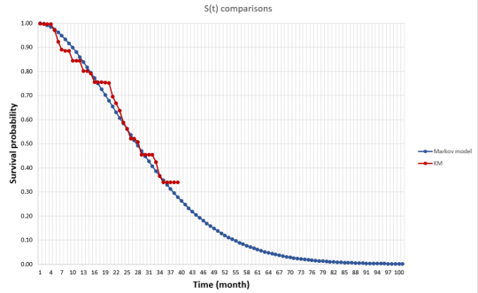
First, when we say survival gain, do we mean median survival or mean survival? Median survival is easier to estimate since you just need to know the median survival for the “typical” person (i.e., someone at the 50th percentile). For mean survival, you would need to know the survival of everyone in the distribution and average over those people. While my research shows that patients generally care most about mean rather than median survival, estimating this is more difficult with clinical trial data. Clinical trials are short and thus one would need to extrapolate survival for all people based on mortality information for a limited number of people for whom we observed death. In the picture below, the line in red is the Kaplan-Meier curve based on clinical trial mortality data and the blue curve is an extrapolation. We can use Kaplan-Meier to calculate the median, but we need the extrapolation to get the mean.

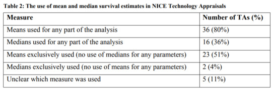
The National Institute for Health and Care Excellence (NICE) has a DSU Technical Document on Survival Analysis for Economic Evaluations. The document examines which types of models are most commonly used. They find that most HTA submissions do use means, but some also will also use median survival estimates as well.

http://nicedsu.org.uk/wp-content/uploads/2016/03/NICE-DSU-TSD-Survival-analysis.updated-March-2013.v2.pdf

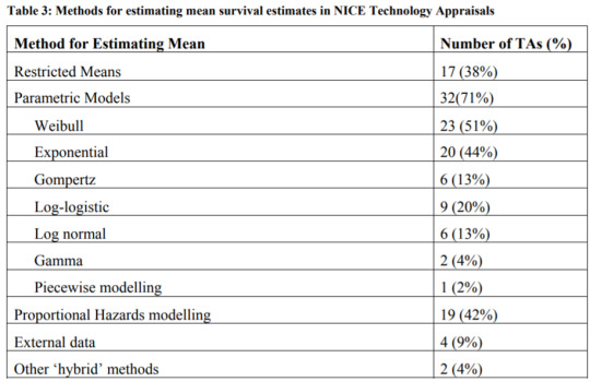
If you need to extrapolate means, how is this most frequently done?

Parametric models are most often used, and the most common ones used for HTA submissions are Weibull and exponential. This is shown in the table below. An exponential distribution assumes a constant proportional hazard and is simplest to estimate. Weibull and Gompertz distributions assume monotonically increasing or decreasing hazard ratios, which adds some flexibility. Log-logistic and lognormal assume an initial increasing hazard and later a decreasing hazard. These last two functions allow to better fit the data when there is a fat tail in the survival distribution, but can overestimate survival if the fat tails are not likely to materialize in practice. The gamma distribution can incorporate all these trends, is the most flexible, but requires estimating more parameters.

http://nicedsu.org.uk/wp-content/uploads/2016/03/NICE-DSU-TSD-Survival-analysis.updated-March-2013.v2.pdf

There are other extrapolation methods such as piecewise models, spine models, cure models, landmark models, or mixture models. However, the NICE document does do a nice job of summarizing the most commonly used approaches for extrapolating survival curves.

from Updates By Dina https://www.healthcare-economist.com/2020/07/24/estimating-survival-gains-based-on-clinical-trial-data/

0 notes

maxihealth · 5 years ago

Text

Estimating survival gains based on clinical trial data

http://nicedsu.org.uk/wp-content/uploads/2016/03/NICE-DSU-TSD-Survival-analysis.updated-March-2013.v2.pdf

If you need to extrapolate means, how is this most frequently done?

http://nicedsu.org.uk/wp-content/uploads/2016/03/NICE-DSU-TSD-Survival-analysis.updated-March-2013.v2.pdf

Estimating survival gains based on clinical trial data posted first on https://carilloncitydental.blogspot.com

0 notes

juniperpublishersoceanography · 3 years ago

Text

Uncertainty Quantification of Sea Waves - An Improved Approach

Abstract

Sea waves are important dynamic loadings for the design of offshore structures. Casual observations will indicate that the sea waves are very unpredictable and may not be modeled deterministically. To capture the unpredictable nature of the sea waves, they are generally expressed in terms of a joint probability density function of mean zero crossing period Tz and the significant wave height Hs. Estimation of parameters of the joint distribution can be very challenging, particularly considering the scarcity of data. The joint probability density function (PDF) of Tz and Hs is generally represented as the multiplication of a conditional distribution for Tz given Hs and the marginal distribution of Hs. The estimation of parameters of the joint PDF is addressed in this paper. The available information on North Atlantic, as reported by Det Norske Veritas (DNV), is considered to document its applicability. DNV reported values for all the required parameters. They are considered as the reference values. Using the Maximum Likelihood Method (MLM), the three parameters of the Weibull distribution for the marginal distribution of Hs are estimated. Assuming Hs can be represented by a two-parameter Weibull distribution, they are also estimated. To compare different alternatives, their Root-Mean-Square-Error values are also estimated. It can be observed that the proposed MLM to estimate the parameters of Hs is superior to that of proposed by DNV.

Read more about this article: https://juniperpublishers.com/ofoaj/OFOAJ.MS.ID.555775.php

Read more Juniper Publishers Google Scholar articles https://scholar.google.com/citations?view_op=view_citation&hl=en&user=V6JxtrUAAAAJ&citation_for_view=V6JxtrUAAAAJ:l7t_Zn2s7bgC

#Juniper Publishers Google Scholar #aquaculture #Marine journals #Fisheries #Marine ecology

0 notes

livingwellpage · 5 years ago

Text

Estimating survival gains based on clinical trial data

http://nicedsu.org.uk/wp-content/uploads/2016/03/NICE-DSU-TSD-Survival-analysis.updated-March-2013.v2.pdf

If you need to extrapolate means, how is this most frequently done?

http://nicedsu.org.uk/wp-content/uploads/2016/03/NICE-DSU-TSD-Survival-analysis.updated-March-2013.v2.pdf

Estimating survival gains based on clinical trial data published first on your-t1-blog-url

0 notes

ijtsrd · 5 years ago

Photo

Estimating the Survival Function of HIV AIDS Patients using Weibull Model

by R. A. Adeleke | O. D. Ogunwale "Estimating the Survival Function of HIV/AIDS Patients using Weibull Model"

Published in International Journal of Trend in Scientific Research and Development (ijtsrd), ISSN: 2456-6470, Volume-4 | Issue-4 , June 2020,

URL: https://www.ijtsrd.com/papers/ijtsrd30636.pdf

Paper Url :https://www.ijtsrd.com/mathemetics/statistics/30636/estimating-the-survival-function-of-hivaids-patients-using-weibull-model/r-a-adeleke

callforpapereconomics, economicsjournal

This work provides information on the survival times of a cohort of infected individuals. The mean survival time was obtained as 22.579 months from the resultant estimate of the shape parameter =1.156 and scale parameter =0.0256 from Weibull 7 simulation of n = 500. Confidence intervals were also obtained for the two parameters at = 0.05 and it was found that the estimates are highly reliable.

#Statistics #Cohort #Survival time #Shape parameter

0 notes

juniperpublishers-robotics-blog · 5 years ago

Text

The Review of Reliability Factors Related to Industrial Robo- Juniper Publishers

Abstract

Although, the problem of industrial robot reliability is closely related to machine reliability and is well known and described in the literature, it is also more complex and connected with safety requirements and specific robot related problems (near failure situations, human errors, software failures, calibration, singularity, etc.).Compared to the first robot generation, the modern robots are more advanced, functional and reliable. Some robot’s producers declare very high robot working time without failures, but there are fewer publications about the real robot reliability and about occurring failures. Some surveys show that not every robot user has monitoring and collects data about robot failures. The practice show, that the most unreliable components are in the robot’s equipment, including grippers, tools, sensors, wiring, which are often custom made for different purposes. The lifecycle of a typical industrial robot is about 10-15 years, because the key mechanical components (e.g. drives, gears, bearings) are wearing out. The key factor is the periodical maintenance following the manufacturer’s recommendations. After that time, a refurbishment of the robot is possible, and it can work further, but there are also new and better robots from modern generation.

Keywords: Industrial robot;Reliability; Failures; Availability; Maintenance; Safety; MTTF; MTBF; MTTR; DTDTRF

Introduction

Nowadays, one can observe the increasing use of automation and robotization, which replaces human labor. New applications of industrial robots are widely used especially for repetitive and high precision tasks or monotonous activities demanding physical exertion (e.g. welding, handling). Industrial robots have mobility similar to human arms and can perform various complex actions like a human, but they do not get tired and bored. In addition, they have much greater reliability then human operators. The problem of industrial robot reliability is like machine reliability and is well known and described in the literature, but because of the complexity of robotic systems is also much more complex and is connected with safety requirements and specific robot related problems (near failure situations, hardware failures, software failures, singularity, human errors etc.). Safety is very important, becausethere were many accidents at work with robots involved, and some of them were deadly. Accidents were caused rather more often by human errors than by failures of the robots.

The research about robot reliability was started in 1974 by Engleberger, with publication, which is a summary of three million hours of work of the first industrial robots–Unimate[1]. A very comprehensive discussion over the topic is presented by Dhillon in the book, which covers the problems of robot reliability and safety, including mathematical modelling of robot reliability and some examples[2]. An analysis of publications on robot reliability up to 2002 is available in Ref. Dhillon et al.[3], and some of the important newer publications on robot reliability and associated areas are listed in the book [4].The modern approach to reliability and safety of the robotic system is presented in the book, which includes Robot Reliability Analysis Methods and Models for Performing Robot Reliability Studies and Robot Maintenance[5]. The reliability is strongly connected with safety and productivity, therefore other researches include the design methods of a safe cyber physical industrial robotic manipulator and safety-function design for the control system or simulation method for human and robot related performance and reliability[6-7]. There are fewer publications about the real robot reliability and about occurring failures [8]. The surveyshows that only about 50 percent of robot users have monitoring and collect data about robot failures.

Failure analysis of approximately 200 mature robots in automated production lines, collected from automotive applications in the UK from 1999, is presented in the article, considering Pareto analysis of major failure modes. However, presented data did not reveal sufficiently fine detail of failure history to extract good estimates of the robot failure rate[9-10].

In the article11. Sakai et al.[11], the results of research about robot reliability at Toyota factory are presented. The defects of 300 units of industrial robots in a car assembly line were analyzed, and a great improvement in reliability has been achieved. The authors consider as significant activities that have been driven by robot users who are involved in the management of the production line. Nowadays, robot manufacturers declare very high reliability of their robots [12]. The best reliability can be achieved by the robots with DELTA and SCARA configuration. This is connected with lower number of links and joints, compared to other articulated robots. Because each additional link with serial connection causes an increase of the unreliability factors, therefore, some components are connected parallel, especially in the Safety Related Part of the Control System (SRP/CS), which have doubled number of some elements, for example emergency stops. Robots are designed in such way that any single, reasonably foreseeable failure will not lead to the robot’s hazardous motion [13].Modern industrial robots are designed to be universal manipulating machines, which can have different sort of tools and equipment for specific types of work. However, the robot’s equipment is often custom made and may turn out to be unreliable as presented in, therefore, the whole robotic system requires periodic maintenance, following to the manufacturer’s recommendations [14-15]. operators and robots in cooperative tasks, therefore, the safety plays a key role. Safety can be transposed in terms of functional safety addressing the functional reliability in the design and implementation of devices and components that build the robotic system [16].

Robot Reliability

The reliability of objects such as machines or robots is defined as the probability that they will work correctly for a given time under defined working conditions. The general formula for obtaining robot reliability is [2]:

Where:

Rr(t) is the robot reliability at time t,

λr(t) is the robot failure rate.

In practice, for description of reliability, in most cases the MTTF (Mean Time to Failure) parameter is used, which is the expected value of exponentially distributed random variable with the failure rate λr [2].

In real industrial environments, the following formula can be used to estimate the average amount of productive robot time, before robot failure [2]:

Where:

PHR – is the production hours of a robot,

NRF – is the number of robot failures,

DTDTRF – is the downtime due to robot failure in hours,

MTTF – is the robot mean time to failure.

In the case of repairable objects, the MTBF (Mean Time Between Failures), and the MTTR (Mean Time to Repair) parameters, can be used.

The reliability of the robotic system depends on the reliability of its components. The complete robotic workstation includes:

A. Manipulation unit (robot arm),

B. controller (computer with software),

C. equipment (gripper, tools),

D. workstation with workpieces and some obstacles in the robot working area,

E. safety system (barriers, curtains, sensors),

F. human operator (supervising, set up, teaching, maintenance).

The robot system consists of some subsystems that are serially connected (as in the Figure 1) and have interface for communication with the environment or teaching by the human operator.The robot arm can have different number of links and joints N. Typical articulated robots have N=5-6joints as in the Figure 2, but more auxiliary axes are possible.

For serially connected subsystems, each failure of one component brings the whole system to fail. Considering complex systems, consisting of n serially linked objects, each of which has exponential failure times with rates λi, i= 1, 2, …, n, the resultant overall failure rate λSof the system is the sum of the failure rates of each element λi[2]:

Moreover, the system MTBFS is the sum of inverse MTBFi, of linked objects:

There are different types of failures possible:

A. Internal hardware failures (mechanical unit, drive, gear),

B. Internal software failures (control system),

C. External component failures (equipment, sensors, wiring),

D. Human related errors and failures that can be:

a. Dangerous for humans (e.g. unexpected robot movement),

b. Non-dangerous, fail-safe (robot unable to move).

Also possible are near failure situations and robot related problems, which require the robot to be stopped and human intervention is needed (e.g. recalibration, reprograming).Because machinery failures may cause severe disturbances in production processes, the availability of means of production plays an important role for insuring the flow of production. Inherent availability can be calculated with the formula 7 [2].

For example, the availability of Unimate robots was about 98 % over the 10-years period with MTBF=500h and MTTR=8 hours [2].

The reliability of the first robot generation represents the typical bathtub curve (as in Figure3), with high rate of early “infant mortality” failures, the second part with a constant failure rate, known as random failures and the third part is an increasing failure rate, known as wear-out failures (it can be described with the Weibull distribution).

Therefore, the standard [17] was provided, in order to minimize testing requirements that will qualify a newly manufactured (or a newly rebuilt industrial robot) to be placed into use without additional testing. The purpose of this standard is to provide assurance, through testing, that infant mortality failures in industrial robots have been detected and corrected by the manufacturer at their facility prior to shipment to a user. Because of this standard, the next robot generation has achieved better reliability, without early failures, with MTBF about 8000 hours [16].In the articleSakai&Amasaka[11], the results of research about robot reliability at Toyota are presented. Great improvement was achieved with an increase of the MTBF to about 30000 hours.

Nowadays, robot manufacturers declare an average of MTBF = 50,000 - 60,000 hours or 20 - 100 million cycles of work [12]. The best reliability is achieved by the robots with SCARA and DELTA configuration. This is connected with lower number of links and joints, compared to other articulated robots.Some interesting conclusions from the survey about industrial robots conducted in Canada in year 2000 are as follows [9]:

A. Over 50 percent of the companies keep records of the robot reliability and safety data,

B. In robotic systems, major sources of failure were software failure, human error and circuit board troubles from the users’ point of view,

C. Average production hours for the robots in the Canadian industries were less than 5,000 hours per year,

D. The most common range of the experienced MTBF was 500–1000h (from the range 500-3000h)

E. Most of the companies need about 1–4h for the MTTR of their robots (but also in many cases the time was greater than 10h or undefined).

The current industrial practice show that the most unreliable components are in the robot’s equipment, including grippers, tools, sensors, wiring, which are often custom made for different purposes. This equipment can be easily repaired by the robot user’s repair department. But the failure of critical robot component requires intervention of the manufacturer service and can take much more time to repair (and can be counted in days). Therefore, for better performance and reliability of the robotic system, periodic maintenance is recommended.

Robot Maintenance

Three basic types of maintenance for robots used in industry are as follows [4]:

Preventive maintenance

This is basically concerned with servicing robot system components periodically (e.g. daily, yearly. …)

Corrective maintenance

This is concerned with repairing the robot system whenever it breaks down.

Predictive maintenance

Nowadays, many robot systems are equipped with sophisticated electronic components and sensors; some of them are capable of being programmed to predict when a failure might happen and to alert the concerned maintenance personnel (e.g. self-diagnostic, singularity detection).Robot maintenance should be performed, following to the robot manufacturer’s recommendations, which are summarized in the Table 1[15]. Preventive maintenance should be provided before each automatic run, including self-diagnostic of the robot control system, visual inspection of cables and connectors, checking for oil leakage or abnormal signals like noise or vibrations. The replacement of the battery, which powers the robot’s positional memory, is needed yearly. If the memory is lost, then remastering (recalibration, synchronization) is needed.Replenishing the robot with grease every recommended period is needed to prevent the mechanical components (like gears) from wearing out. Special greases are used for robots (e.g. Moly White RE No.00) or grease dedicated for specific application like for the food-industry. Every 3-5 years a fully technical review (overhaul) with replacement of filters, fans, connectors, seals, etc. is recommended.

Performing daily inspection, periodic inspection, and maintenance can keep the performance of robots in a stable state for a long period. The lifecycle of typical robot is about 10-15 years, because the wear of key mechanical components (drives, gears, bearings, brakes) causes backlash and positional inaccuracy. After that time a refurbishment of the robot is possible, and it can work further for long time. Refurbished Robots are also called remanufactured, reconditioned, or rebuilt robots.

Conclusion

Nowadays modern industrial robots have achieved high reliability and functionality;therefore, they are widely used. This is confirmed by more than one and half million of robots working worldwide. According to the probability theory, in such large robot population the failures of some robots are almost inevitable. The failures are random, and we cannot predict exactly where and when, they will take place. Therefore, the robot users should be prepared and should undertake appropriate maintenance procedures. This is important, because industrial robots can highly increase the productivity of manufacturing systems, compared to human labor, but every robot failure can cause severe disturbances in the production flow,therefore periodic maintenance is required, in order to prevent robot failures. High reliability is also important for the next generation of collaborative robots, which should work close to human workers, and safety must be guaranteed without barriers. Also, some sorts of service robots, which should help nonprofessional people (e.g. health care of disabled people) must have high reliability and safety. There have already been some accidents at work, with robots involved, therefore, the next generation of intelligent robots should be reliable enough to respect the Asimov’s laws and do not hurt people, even if they make errors and give wrong orders.

For More Open Access Journals Please Click on: Juniper Publishers

Fore More Articles Please Visit: Robotics & Automation Engineering Journal

#Juniper Publishers #Robotics #Open Access Journals #Self Ruling Robots #Machine Learning

0 notes

craigbrownphd-blog-blog · 6 years ago

Text

R Packages worth a look

Density Estimation for Extreme Value Distribution (DEEVD) Provides mean square error (MSE) and plot the kernel densities related to extreme value distributions. By using Gumbel and Weibull Kernel. See Salha et … User Friendly Bayesian Data Analysis for Psychology (bayes4psy) Contains several Bayesian models for data analysis of psychological tests. A user friendly interface for these models should enable students and resear … Derive MCMC Parameters (mcmcderive) Generates derived parameter(s) from Monte Carlo Markov Chain (MCMC) samples using R code. This allows Bayesian models to be fitted without the inclusio … Yet Another TAxonomy Handler (yatah) Provides functions to manage taxonomy when lineages are described with strings and ranks separated with special patterns like ‘|*__’ or ‘;*__’. http://bit.ly/2oKdS84

0 notes

jccamus · 6 years ago

Text

Influence of Money Distribution on Civil Violence Model

Influence of Money Distribution on Civil Violence Model https://ift.tt/2J6xXfC

Abstract

We study the influence of money distribution on the dynamics of Epstein’s model of civil violence. For this, we condition the hardship parameter distributed according to the distribution of money, which is a local parameter that determines the dynamics of the model of civil violence. Our experiments show that the number of outbursts of protest and the number of agents participating in them decrease when the distribution of money guarantees that there are no agents without money in the system as a consequence of saving. This reduces social protests and the system shows a phase transition of the second order for a critical saving parameter. These results also show three characteristic regimes that depend on the savings in the system, which account for emerging phenomena associated with the saving levels of the system and define scales of development characteristic of social conflicts understood as a complex system. The importance of this model is to provide a tool to understand one of the edges that characterize social protest, which describes this phenomenon from the sociophysics and complex systems.

1. Introduction

In the last decades, different studies have been carried out that seek to describe the society in the framework of complex systems [1]. One of the most used modeling approaches is the so-called bottom-up [2]. This approach is characterized by the use of agent-based models (MBAs) to reproduce artificial worlds or virtual societies and has been widely used to describe sociological phenomena such as the dynamics of segregation [3] and cultural diffusion [4]. A further review of these topics is found in the books of Epstein [5, 6].

Social conflicts have been characterized as emergent properties of a complex system that depends on the scale and levels at which they occur [7], resulting in protests, civil violence, wars, or revolutions. The use of variations of the model proposed by Epstein [8] has allowed describing different scenarios of social unrest, such as workers’ protests due to wage inequality [9], propagation and persistence of criminal activity in the population [10], or cases of civil war between ethnic groups due to their geographical distribution [11]. Moreover, authors have worked on variants of the Epstein model [8] that have led to increasing the complexity of the dynamics. A class of models with this characteristic is achieved by adding more variables to the dynamics. Other models incorporate strategies into agents’ decisions, such as allowing agents to gain learning using game theory or collective coevolution given by the interaction between agents [12]. There are also models where one of the parameters that define dynamics, such as legitimacy, has endogenous feedback [13].

To interpret the results obtained in the simulations, it is appropriate to use the concepts and tools of statistical physics. This fact has given rise to branches or new fields of interdisciplinary research [14–16] such as the econophysics [17–20] and the sociophysics [21–23]. Econophysics studies and describes statistical properties of economic systems with large amounts of economic and financial data through the use of techniques and tools originally developed in statistical physics [18]. In sociophysics the social behavior is described making use of the physics of the critical phenomena, emphasizing, among these, the use of the theory of phase transitions to describe social, psychological, political, and economic phenomena [24–27].

The goal in this paper is to study the dynamics of civil violence when the money distribution is taken into consideration. For this we condition the hardship parameter distributed according to the money distribution, unlike the Epstein model [8] where it is uniformly distributed. The distribution of money is a result of the dynamics of money exchange between agents with a propensity to save money, as obtained in [28, 29]. In this way, we can study the influence of inequality in the money distribution of the society in the emergence of social mobilizations.

The order in which the contents are presented will be as follows. In Section 2, we will briefly describe the models used for the simulations and the elements that compose the comparative study. Then, in Section 3, we present the results obtained; then, in Section 4, we conduct the discussion and establish the conclusions.

2. Civil Violence Model

This agent-based model [8] simulates a process of social protest to which authority responds with the use of force to restore public order. The dynamic is established by relating the legitimacy of authority and the hardship of agents to the discontent of the population. The general state of the system is determined by global variables such as the legitimacy , the vision of the agents , the maximum sentence , and a state evaluation threshold .

The agents, citizens, and police are placed at random on a rectangular grid with periodic edge conditions. The dynamics of the agents is achieved with decisions made taking into account the information obtained within the neighborhood of each agent selected. The neighborhood extension is defined by the range of vision of each agent. Citizens are agents that are characterized by two parameters: hardship and risk aversion . These quantities are assigned to the agents as uniformly distributed random values. With these parameters and according to the evaluation of local conditions, each agent will decide whether or not to join the protest. To do this, each agent evaluates its state by means of its grievance and its net risk , where is the probability of arrest that is obtained based on a number of active agents and police in your neighborhood.

Thus, the active state indicates that the agent joins the protest and the passive state is when the agent stays on the sidelines. On the other hand, the police are agents that do not have parameters assigned and are responsible for restoring order by capturing the active agents who are in their neighborhood defined by their vision.

The rules that determine the dynamics of the model are the following:(1)Rule of motion: it is valid for all agents and allows them to move to an empty space at random within their neighborhood.(2)The rule of state evaluation: it is given by . Citizens who comply with this rule transform their status from a passive agent to an active agent; otherwise, the agent will remain a passive agent.(3)Capture rule: cops randomly capture an active agent from among the active agents in their neighborhood and move to that location on the grid. In case there are no active agents, they do nothing.

Epstein, to determine the existence of emerging phenomena, which he defines as “macroscopic regularities arising from the pure local interaction of agents” [2], proposes to study the waiting times distribution between each outburst and distribution of their sizes.

For the study of waiting times, Epstein defines a threshold of 50 active agents to consider the event as an outburst, where the outburst size is defined as the maximum amount of active agents during the event. Based on simulations carried out with iterations, Epstein finds that the waiting times distribution corresponds to a log-normal distribution, while the outburst size distribution corresponds to a Weibull distribution [8].

Table 1 lists the global and local parameters used to reproduce the results reported by Epstein [8]. The size of the grid is and has toroidal topology, agent density is , police density is , and the probability of arrest is .

Table 1:

Global and local parameters used to reproduce the results reported by Epstein [

]. The size of the grid is (40 × 40) and has toroidal topology, agent density is 0.7, police density is 0.04, and the probability of arrest is

Figure 1 shows the results obtained when reproducing the Epstein [8] model. Panel (a) shows the temporal evolution of the number of agents participating in a protest. The red line represents the number of active agents in the system. The observed events correspond to the phenomenon of punctuated equilibrium [30]. In panel (b), the histogram of the waiting times is displayed, while in panel (c), the histogram of the outburst sizes is displayed. For these results, we considered experiments of iterations and the parameters shown in Table 1.

Figure 1:

Results obtained when reproducing the model of Epstein [

]. Panel (a) shows the temporal evolution of the number of agents participating in a protest. The red line represents the number of active agents in the system. The observed events correspond to the phenomenon of punctuated equilibrium [

]. In panel (b), the histogram of the waiting times is displayed, while in panel (c), the histogram of the outburst sizes is displayed. For these results, we considered

experiments of

iterations and the parameters shown in Table

3. Money Distribution Models

At the end of the 90s, studies were conducted on the distribution of money, income, and wealth to describe the dynamics of economic systems by modeling commercial transactions such as the interactions between the molecules of a gas where they exchange momentum and energy. Therefore, they are appropriately described by the use of tools of statistical physics [18–20].

In particular, the results obtained with gas-like models [28, 29, 31, 32] have allowed the researchers to establish a parallel with a thermodynamic system closed in thermal equilibrium, where the agents exchange an amount of money as the particles of a gas in a closed system exchange momentum and energy. This analogy is possible since ordinary economic agents can only exchange money with other agents. They are not allowed to “make” money, for example, printing dollar bills [32]. In a system of agents that perform exchanges that fulfill the condition of time reversal, the distribution of money corresponds to the distribution of Boltzmann-Gibbs [32]. With these considerations, we can use the canonical ensemble to perform the physical description and obtain the probability function associated with an amount of money and with this know the distribution of this in the system.

In this paper, we use the results obtained from the dynamics of money exchange in the case that all agents save a portion of their money at the moment of making a money transaction and of the remaining amount the agents exchange a random fraction of it [28].

Thus, we have a system with total money and agents, which initially have an equal amount of money. The saving factor is homogeneous in the system. The exchange of money between agents obeys the equation , where the fraction being exchanged is given by where is a random number with a uniform distribution between zero and unity. Note that when the agents do not save (), we retrieve the Boltzmann-Gibbs distribution obtained in the work of Dragulescu and Yakovenko [32]. When the saving is different from zero (), a money distribution is similar to the gamma distribution [31].

Second, we will use the description of Chatterjee et al. [29], in which the saving factor is different for all agents and evenly distributed, that is, a heterogeneous factor in the system. In this case, the fraction being exchanged is given bywhere the saving factors for each agent , , and are uniformly distributed random values between and . The result of this configuration gives a money distribution given by a mixture between a Boltzmann-Gibbs distribution and a Pareto, which is very close to the results reported in the analysis made to real wealth distribution and income data [29, 33].

In Figure 2, the results obtained by reproducing the distributions of money obtained in [29, 31] are shown. In panel (a), the money distributions are shown for cases where saving is a homogeneous feature in the system. The blue circles show the boundary case with , which corresponds to an exponential distribution as reported in [32]. The cases with are shown with circles of red, green, yellow, and magenta, respectively. These results correspond to a gamma distribution as reported in [31]. In panel (b), the money distribution for distributed heterogeneously in the system is shown, which corresponds to a Pareto distribution as reported in [29]. To obtain these results, agents with initial money and were considered.

Figure 2:

Results obtained by reproducing the distributions of money obtained in [

]. In panel (a), the money distributions are shown for cases where saving is a homogeneous feature in the system. The blue circles show the boundary case with

, which corresponds to an exponential distribution as reported in [

]. The cases with

are shown with circles of red, green, yellow, and magenta, respectively. These results correspond to a gamma distribution as reported in [

]. In panel (b), the money distribution for

distributed heterogeneously in the system is shown, which corresponds to a Pareto distribution as reported in [

4. Epstein Model Conditioned by the Money Distribution of Agents with Propensity to Save

In order to study the influence of the money distribution on the emergence of social mobilizations we modified the hardship parameter that in the model civil violence is evenly distributed through the following expression:where is the amount of money of the agent and is the amount of money of the richest agent in the system. Thus, the preparation of the numerical experiments with this hybrid model is carried out following the steps indicated below:(1)It is assigned initial values for each parameter, both local and global.(2)At the beginning of the procedure, economic exchanges are carried out between agents to obtain the money distribution. This number of iterations is above the number of iterations necessary to reach the constant entropy regime in the system. In this process of exchange of money, only the agents of citizen type participate. Agents with the role of police do not participate in the exchange of money nor do they evaluate the state nor participate in the protests.(3)The distribution of hardship is obtained from the distribution of money by means of (3).(4)The simulation of civil violence begins.

In this study to obtain the average results of each case shown, experiments of iterations each were carried out. In our study, we consider two cases in relation to the legitimacy parameter, : the case with as in Epstein and the case with . The latter corresponds to the value obtained after rescaling the legitimacy by taking the mean value of the state evaluation rule obtained with both the hardship uniform distribution parameter and the hardship parameter obtained with the money distribution. In Table 2, the parameters used in both cases are shown.

Table 2: Global and local parameters used in the simulations for Case I (a) and Case II (b). The grid dimensions are , its topology is toroidal, the agent density is , the police density is , and the arrest probability constant is .

Following the analysis made for the model of civil violence, for each case, we will present the distributions of waiting times and sizes of the outbursts. To compare the results of the Epstein model with the present hybrid model, we used outburst quantity, waiting times, and outburst sizes.

5. Results of the Simulations

First, we perform simulations of the model conditioned by the distribution of money with the parameters of the original Epstein model (see Table 2).

In Figure 3(a), the change of the distribution of the waiting times according to the saving parameters is shown, which are drawn with lines and circles of red, green, yellow, black, magenta, and cyan, respectively. The line with squares in blue corresponds to the case with heterogeneous saving in the system, while the line with blue circles corresponds to the distribution obtained with the original Epstein model. In Figure 3(b), the changes in the size distribution of the burst are shown for the saving parameters , which are drawn with lines and circles of red, green, yellow, black, magenta, and cyan, while the blue line with squares corresponds to the case with heterogeneous saving in the system. The blue line with circles corresponds to the Epstein model.

Figure 3: (a) Distribution of waiting times. The change of the distribution of the waiting times according to the saving parameters is shown, which are drawn with lines and circles of red, green, yellow, black, magenta, and cyan, respectively. The line with squares in blue corresponds to the case with heterogeneous saving in the system, while the line with blue circles corresponds to the distribution obtained with the original Epstein model. (b) Distribution of burst sizes. The changes in the size distribution of the burst are shown for the saving parameters , which is drawn with lines and circles of red, green, yellow, black, magenta, and cyan, while the blue line with squares corresponds to the case with heterogeneous saving in the system. The blue line with circles corresponds to the Epstein model.

In Figure 3(a) it can be observed that, for the case of heterogeneous distribution of savings, the short waiting times are more frequent, the reason why the system is at its maximum activity. The same characteristic is observed for the case of zero saving, where the highest frequency is obtained for short times. As the saving parameter increases, the maximum frequency of the waiting times decreases progressively and occurs at similar waiting times greater than for cases of heterogeneous saving and zero saving. The dynamics obtained in the Epstein model is closer to cases of high savings factor. In Figure 3(b), as in the case of waiting times, cases of heterogeneous saving and zero saving have the maximum frequencies for large outburst sizes. As the saving parameter increases, the frequency maxima decrease and take place for smaller outburst sizes. For the case of Epstein, it is observed that the maximum of the frequencies is in outburst sizes similar to the case with saving .

In Figure 4(b), we observe how the waiting time between each burst increases as the saving increases. As in Figure 4(a), there is a strong increase in waiting times from savings. For , no bursts are observed during the simulation time of iterations.

Figure 4: (a) The outburst quantity is plotted according to the saving parameter. With the line with red squares, the outburst quantity is graphed. The blue circle corresponds to the value obtained with the Epstein model, while the green diamond corresponds to the value obtained for the case with heterogeneous savings. (b) The waiting times are plotted according to the saving parameter. The line with red squares shows the time between each outburst for homogeneous . The blue circle corresponds to the value obtained with the Epstein model and the green diamond corresponds to the value obtained for the case with heterogeneous savings.

In Figure 4(a), the outburst quantity is plotted according to the saving parameter. With the line with red squares, the outburst quantity is shown. The blue circle corresponds to the value obtained with the Epstein model, while the green diamond corresponds to the value obtained for the case with heterogeneous savings. In Figure 4(b), the waiting times are plotted according to the saving parameter. With the line with red squares, the time between each outburst is plotted. The blue circle corresponds to the value obtained with the Epstein model and the green diamond corresponds to the value obtained for the case with heterogeneous savings. It is observed from Figure 4(a) that the outburst quantity decreases continuously as savings increase, approaching zero when , resulting in a phase transition. For cases of , the absence of outbursts is observed; that is, the punctuated equilibrium disappears giving rise to a regime that can be characterized as noise (as we shall see later), being the activity of active agents under the threshold for a burst. In Figure 4(b), we observe how the waiting time between each burst increases as the saving increases. As in Figure 4(a), there is a strong increase in waiting times from savings. For , no bursts are observed during the simulation time of iterations.

In Figure 5(a), the outburst sizes are plotted against the savings. The red lines show the average value of the size of the outburst in the range , where is the standard deviation of the maximum values of the outburst sizes for each lambda value. The magenta and cyan lines show the average value of the size of the outbursts above and below the range , respectively. The blue circle corresponds to the average size of the outbursts obtained for the Epstein model and the diamond the average size of the outbursts obtained with heterogeneous lambda. Figures 5(b), 5(c), and 5(d) show the average value of the size of the outbursts with their corresponding error bars, obtained both in the range and over and under the range, respectively.

Figure 5: (a) The outburst size is plotted against the savings. The lines with red squares show the average value of the size of the outburst in the range , where is the standard deviation of the maximum values of the outburst sizes for each lambda value. The magenta and cyan lines show the average value of the size of the outbursts above and below the range , respectively. The blue circle corresponds to the average size of the outbursts obtained for the Epstein model and the diamond the average size of the outbursts obtained with heterogeneous lambda. In panels (b), (c), and (d), the average value of the size of the outbursts with their corresponding error bars, obtained both in the range and over and under the range, respectively.

As can be seen in Figure 5, the outburst size decreases similar to outburst quantity (see Figure 4) with the occurrence of three regimes for the maxima at each outburst. The lower intensity maxima (see Figure 5) correspond to outbursts that are not completely quenched, leaving a remnant of active agents large enough to generate a resurgence of the outburst, disappearing when . Outbursts with maximum values above range (see Figure 5(c)) appear as approaches 0.7 and vanish as approaches 0.80.

The existence of these three regimens for the maxims of each outburst implies that the dynamics obtained with the model dependent on the distribution of money does not correspond rigorously to the punctuated equilibrium, as described by Bak and Sneppen [30] and Epstein [8].

The simulations performed so far use the legitimacy value of the original Epstein model. From Figures 3, 4, and 5, we can see that the sizes, the quantity of the outburst, and the waiting times for the case , that is, when the distribution of hardship is exponential, are notoriously greater than for the case of Epstein. The uniform hardship distribution has a smaller number of active agents than the exponential case. Clearly, the legitimacy of society in both cases cannot be the same.

In order to obtain a system with comparable dynamics to the Epstein model, in terms of outburst sizes, outburst quantity, and waiting times, we take the mean value of the equation that establishes the rule of state evaluation, to give where is the average grievance of the system for the model under the parameters of Epstein and is the average grievance for the savings-dependent system . Then,

Equation (5) allows us to obtain a value of the rescaled legitimacy that gives us the possibility of making the dynamics of the systems under discussion comparable. In Table 3, the average value of the hardship, , and the rescaled legitimacy, , are shown for each saving factor value, . The value used in Epstein for legitimacy is and the mean value of the hardship is ( is a random variable evenly distributed between and ). From Table 3, it is read that the rescaling value of the appropriate legitimacy is . With the value for the rescaled legitimacy, the simulations are repeated with the general parameters shown in Table 2.

Table 3: The averages for and for each obtained with the data generated for Case I.

As seen in Figure 6(a), in all distributions, the maximum frequency takes place for wait times of the order of . In contrast to what is observed in Figure 3(a) with Epstein’s legitimacy, cases of heterogeneous savings and show the same characteristic as cases of homogeneous saving, having a maximum of frequency in standby time . Like what is observed in Figure 3(a), all cases differ in the maximum value of the frequency. Likewise, the higher frequency is obtained when the distribution of savings is heterogeneous. The result of the rescaling produces that the maximum frequency for the Epstein case is greater than those obtained for cases with homogeneous savings. For the outburst sizes distribution (see Figure 6(b)), the case with heterogeneous saving has the largest sizes and frequency of outbursting. The cases where the agents are willing to save have both size and the maximum value of the outburst frequency decreasing for values of decreasing outburst size and the saving factor increases. The maximum frequency in the case studied by Epstein is similar to the maximum of the frequency in the outbursts size for the case with saving factor , but with an outburst frequency very similar to the heterogeneous case.

Figure 6: (a) The waiting time distribution with rescaled legitimacy. (b) The outburst sizes distribution with rescaled legitimacy for saving parameters is plotted. The cases with homogeneous saving are drawn with red, green, yellow, magenta, and cyan lines for the values, respectively. The line with squares in black corresponds to the case with heterogeneous saving in the system, while the line with blue circles corresponds to the distribution obtained with the original Epstein model.

In Figure 7(a), the outburst quantity is plotted as a function of the saving parameter with the rescaled legitimacy. With the line with red squares, the quantity of outburst is plotted, while the blue circle corresponds to the value obtained with the Epstein model and the green diamond corresponds to the value obtained for the case with heterogeneous saving. In Figure 7(b), the waiting times are shown as a function of the saving parameter with the rescaled legitimacy. With the line with red squares, the time between each outburst is plotted as the blue circle corresponds to the value obtained with the Epstein model and the green diamond corresponds to the value obtained for the case with heterogeneous saving. In the case with , a continuous decrease in the number of outbursts is observed, and the factor of savings of the agents is increased. Unlike the case with , when , the outbursts are not observed from . Note the sensitivity of the appearance of outburst to the value of legitimacy.

Figure 7: (a) The outburst quantity and (b) the waiting times are shown as a function of the saving parameter with the rescaled legitimacy. The line with red squares shows the time between each outburst for homogeneous . The blue circle corresponds to the value obtained with the Epstein model and the green diamond corresponds to the value obtained for the case with heterogeneous saving.

It is observed how the time between each outburst increases as savings increase, and consistently with the outbursts quantity (see Figure 7(b)), there is a sustained increase in waiting times up to savings. From the value , the absence of outbursts in the simulation time is observed.

In Figure 8(a), the outburst sizes are plotted against the savings. The red line shows the average value of the size of the outburst in the range , where is the standard deviation of the maximum values of the outburst sizes for each value of . The magenta and cyan lines show the average value of the size of the outbursts above and below the range , respectively. The blue circle corresponds to the average size of the outbursts obtained for the Epstein model and the diamond corresponds to the average size of the outbursts obtained with heterogeneous lambda. In Figures 8(b), 8(c), and 8(d), the average value of the size of the outbursts with their corresponding error bars, obtained both in the range and above and below the range, respectively, is plotted in detail.

Figure 8: (a) The outburst sizes depending on the savings. The lines with red squares show the average value of the size of the outburst in the range , where is the standard deviation of the maximum values of the outburst sizes for each value of . The magenta and cyan lines show the average value of the size of the outbursts above and below the range , respectively. The blue circle corresponds to the average size of the outbursts obtained for the Epstein model and the diamond the average size of the outbursts obtained with heterogeneous lambda. In Figures (b), (c), and (d) the average value of the size of the outbursts with their corresponding error bars, obtained both in the range and over and under the range, respectively.

As can be seen in Figure 8, the size of the outburst similarly decreases as the number of outbursts (see Figure 7); in the absence of outburst it is from . Again we have the appearance of three regimes of the maxima in each outburst as in Figure 5, the maxima of lower intensity (see Figure 8(d)), and the outbursts with maximum values above the range (see Figure 8(c)) .

By introducing the money-dependent hardship parameter, the outburst quantity produced in the system continuously decreases as agent savings increase as can be seen in Figure 4(a). This behavior is characteristic of a second-order phase transition, according to the classification criteria found in the literature [34]. As the outbursts decrease, the regularity with which they occur also decreases, which implies an increase in the waiting times between the outbursts; the results can be observed in Figure 4(b). In the same way that the outburst quantity decreases with the increase in savings in the system, the outburst size also decreases, which can be seen in Figure 5(b). Note that in Figures 5(c) and 5(d) there are both outbursts on average as well as under average, which indicates that there are different dynamics associated with outbursts. There are events where active agents have better conditions in their neighborhood to join a protest generating a burst above average. On the other hand, outbursts below average respond to smaller outbursts that come after a major outburst, so it can be interpreted as a replica of the previous main outburst. These subsequent events are due to the fact that at the end of the main outburst the most active agents are not captured, which are reactivated by improving the conditions in their neighborhood, producing a second successive outburst.

These results can be observed at the macroscopic level by looking at the distributions of the wait times in Figure 3(a) as well as in the outburst sizes distribution Figure 3(b). In the case of waiting times, we can see that as the savings increase in the system, the value associated with the more frequent time is increasing, as well as a deformation of the distribution due to the fact that the outburst decreases in both their regularity and quantity. For the outburst sizes distribution, it is observed that the most frequent size decreases as savings increase, which causes a deformation of the distribution both in its more frequent values and also in its form, showing how the dynamics of the outbursts change as they cease to occur.

The results obtained for simulations with were the same results described for . However, the disappearance of the outbursts with occurs for unlike the case with occurring for . This is because increasing legitimacy, , decreases the grievance of each agent, which generates a decrease in the group of agents that could change their status given the conditions in their neighborhood. As a result, the activity of active agents can be reduced by imposing fewer savings in the system. That is to say that the more legitimate the system is, the less we need to save as a redistributive factor to reduce social protests.

Figure 9 shows the power spectrum of a number of active agents during a simulation with , using the Fourier transform. In blue we have the result obtained for the model of Epstein and in green the one corresponding to the simulation with heterogeneous saving. In red the cases for the homogeneous saving model are plotted with , respectively. The dashed lines show the region of the frequency range used to obtain the slope of the decay of the energy cascade in the inertial range. Spectra are observed to occur in the same frequency range . In the low frequency range, an increase in energy is observed as a consequence of the increase of the active agents in the system. The second range, at intermediate frequencies, presents energy cascades characteristic of turbulent phenomena [35].

Figure 9: The power spectrum of a number of active agents during a simulation with , using the Fourier transform. In blue we have the result obtained for the model of Epstein and in green the one corresponding to the simulation with heterogeneous saving. In red the cases for the homogeneous saving model are plotted with , respectively. The dashed lines show the region of the frequency range used to obtain the slope of the decay of the energy cascade in the inertial range.

In Figure 9(a), the spectral power of the number of active agents for the studied cases is shown. It is observed that the spectrum obtained for the Epstein model develops near in the spectral power range, whereas for the heterogeneous saving model it is of similar characteristics as the cascade obtained for the saving model with since they are developed in the same ranges of spectral power. This indicates that the system in these cases behaves similarly and has the same amount of energy. Comparing these cases with the spectrum of the Epstein model, we verified that the dynamics in these models are different from the dynamics of the punctuated equilibrium, as we observed in Figure 5. This behavior remains for the model with homogeneous saving until , to arrive at the case with where the spectrum develops in the same ranges of the spectral power for the case of Epstein model. This indicates that the spectral power for the cases with savings between and decreases until reaching the spectral power associated with the dynamics of the punctuated equilibrium. Then, it is observed that for the model with homogeneous savings between and , it decreases rapidly, arriving at the case with , where the spectrum obtained is characteristic of the white noise. These results are consistent with those shown in Figures 4 and 5, where the absence of outburst is reported near .

The power spectrum of the number of active agents obtained during a simulation for the case with is shown in Figure 10. The blue color corresponds to the power spectrum obtained for the Epstein model; in green color the spectrum of power corresponds to the simulation with heterogeneous saving. In red color, the power spectrum is drawn for the cases for the homogeneous saving model with ], respectively. The region between the segmented lines shows the frequency range used to obtain the slope of the decay of the energy cascade in the inertial range. This figure shows the same behavior described in Figure 9, but resumes the dynamics of the punctuated equilibrium.

Figure 10: The power spectrum of a number of active agents obtained during a simulation for the case with is shown. The blue color corresponds to the power spectrum obtained for the Epstein model; in green color the spectrum of power corresponds to the simulation with heterogeneous saving. In red color, the power spectrum is drawn for the cases for the homogeneous saving model with ], respectively. The region between the segmented lines shows the frequency range used to obtain the slope of the decay of the energy cascade in the inertial range.

Figure 11(a) shows the slope associated with the cascade of the power spectrum as a function of the saving parameter with and in Figure 11(b) the results corresponding to the simulations with are shown. With red squares the slope is drawn for the model with homogeneous saving; the blue circle corresponds to the value obtained with the Epstein model, while the green diamond is the result for the slope in the model with heterogeneous saving. In this figure, it is observed that the value of the slope obtained for the energy cascade of the Epstein model, for both cases, corresponds to the behavior of power law .

Figure 11: (a) shows the slope associated with the cascade of the power spectrum as a function of the saving parameter with and in (b) the results corresponding to the simulations with are shown. With red squares, the slope is drawn for the model with homogeneous saving, and the blue circle corresponds to the value obtained with the Epstein model, while the green diamond is the result for the slope in the model with heterogeneous saving.

In Figure 11(a), it can be seen that the slope value for the heterogeneous model has the same value as for the case with homogeneous savings with , which is evidence that the dynamics are similar. There are three clear behaviors (states); the first is where the value of the slope for the case with homogeneous saving stays almost constant up to , and then there is a decrease in the value of slopes in a sustained way up to , where its value is close to the value obtained with the Epstein model, which indicates that the energy and the dynamics of the punctuated equilibrium are recovered. Then for values between and , a progressive increase in the value of the slopes is observed until values close to zero are reached, indicating that the slope disappears and the spectrum associated with the white noise is obtained, as we can see in Figure 10(f). In the first state, the spectrum has a behavior of type own log-normal distributions, in the second state the spectrum is turbulent, and in the last state there is no dependence of .

In Figure 11(b), it can be seen that the slope value obtained for the heterogeneous model is larger than for the homogeneous savings model of . Then it can be seen that, for , the slope value is similar to that obtained for the Epstein model, which indicates the recovery of the punctuated equilibrium. Then, from , the slope value begins to decrease to zero in the lambda values of and , where the power spectrum already has white noise characteristics.

These results show the existence of three characteristic regimes that depend on the savings in the system. The first scheme is given between and when and for with . This is characterized by a wave of successive protests, a product of the replicas generated by a lot of active agents in the system. From the power spectrum, it is observed that there is a greater amount of energy in the system in this scheme. The second regime is punctuated equilibrium, characteristic of the Epstein model. This phase of the system is obtained by increasing the savings to , when and for with . Evidence of this is the power law that appears in the power spectrum. The last regime is the absence of burst, between and when and from with . This is characterized by having activity under the threshold defined for an outburst, which is observed in the power spectrum as white noise. These regimes account for emerging phenomena associated with system savings levels and define scales of development characteristic of social conflicts understood as a complex system [7].

6. Conclusions

In this paper, we study the influence of the distribution of money on the emergence of social mobilizations using the dynamics of Epstein’s civil violence model conditioned through the hardship parameter distributed according to the distribution of money with savings [28, 29] between agents. Our experiments show that hardship is one of the determining factors for the model of civil violence and this model, so its association to the distribution of money is fundamental to establish a variation of the dynamics.

In the cases we have analyzed, we find that the outbursts quantity and the number of active agents are decreasing as the saving factor increases. Let us assume the average quantity of outbursts as an order parameter. This determines a change of a phase characterized by very regular outbursts of protest to another one characterized by the absence of outbursts. The order parameter varies continuously vanishing at the critical point for a critical value of the saving parameter . This behavior is characteristic of a second-order phase transition, according to the classification criteria found in the literature [34]. Moreover, the critical value of the saving parameter, , depends on the legitimacy parameter, . Our results show that when legitimacy increases, the outbursts disappear with a much lower critical value of the saving parameter. This also indicates that the more legitimacy the authority has in the system, the fewer savings are needed as a redistributive factor to reduce social protests.

These results show three characteristic regimes that depend on the savings in the system. The first regime is characterized by a wave of successive protests and more energy is observed in the system. The second regime is punctuated equilibrium, characteristic of the Epstein model. The last regime is the absence of outbursts. These regimes account for phenomena associated with the savings levels of the system and define scales of development characteristic of social conflicts understood as a complex system [7].

The importance of this model is to provide a tool to understand one of the edges that characterize social protest, which adds to other efforts made [9–11, 13] to describe this phenomenon from other points of view. Undoubtedly, to understand this phenomenon in depth it is possible to establish more parameters that determine unhappiness, such as emotional, cultural, or other factors, which allows for more realistic approaches to the cost of making the model more complex, which will be addressed in future works.

Conflicts of Interest

The authors declare no conflicts of interest regarding the publication of this manuscript.

https://ift.tt/2wvf3KA via Hindawi October 19, 2019 at 10:06PM

#IFTTT #Feedly

0 notes