#correlation coefficient r

[nickfoxer]

Why a Spinoff for Tarlos Is Feasible,Based on AO3 Data.

In this article,I will explain why the decline in Tarlos'popularity is an illusion and why Tarlos'popularity is rebounding and has a solid and reliable core audience in the long term.

It is well-known in American TV shows that the popularity of a ship is reflected in the annual increase of AO3 tags.The popularity of a ship is associated with many factors,such as the director's skills,the scriptwriter's plot design,and the chemistry between actors.

When the director,scriptwriter,and production team remain the same across seasons of the same TV show,these factors may fluctuate but the changes are relatively small.In such cases,people often overlook a key factor affecting the annual increase of AO3 tags:the number of episodes aired in a season!

(Top 100 in 2021,2022 and 2023)

For example,in 2023,compared to 2024,the annual increase of AO3 tags for"TK/Carlos"declined and exited the top 100 for the first time since 2021.Does this mean Tarlos is no longer popular?On the contrary,the conclusion is incorrect because it ignores the number of episodes aired each season.

9-1-1:Lone Star from 2020 to 2023,each year saw a complete season aired,while only nine episodes were broadcast in Season 5 in 2024.

According to the Pearson correlation coefficient formula,the annual increase of tags is strongly positively correlated with the total number of episodes per year(referred to as"episodes").

The correlation coefficient : r≈ 0.645

In statistics,when 0.7≤|r|≤ 1,two factors are considered to have a strong correlation.However,from Seasons 1 to 4,there were fluctuations in production quality.Season 4 had the lowest ratings on various review websites compared to the previous three seasons.Did this fundamental factor affect the tag increase in 2023?

To test this hypothesis,we removed the data from Season 4 and recalculated the Pearson correlation coefficient using data from Seasons 1,2,3,and 5.

The new correlation coefficient：r'≈ 0.845

We then conducted a hypothesis test to verify the p-value:(0.05<p<0.1),which means the correctness rate of the correlation is over 90%.

Thus,under similar production standards,the number of episodes in9-1-1:Lone Starand the annual increase of"Carlos/TK"AO3 tags have a very strong positive correlation.

We can conclude that the main reason for the drop of"TK/Carlos"out of the top 100 in 2024 was the reduced number of episodes aired that year.

Apart from statistical analysis,other factors also played a role:

1. Season 5 premiered at the end of September.By the cutoff date for the rankings(January 1,2025),only nine episodes had been aired.Many viewers hadn't had time to watch,and many fan fiction authors hadn't had time to write.

2. Previous seasons(Seasons 1-4)were broadcast at the beginning or middle of the year,finishing by September at the latest.They attracted viewers for most of the year.In contrast,Season 5 only had three months(from September to December)to attract viewers.

3. The gap between the premiere of Season 5 and the last episode of the previous season was as long as 13 months,longer than the gap between any other seasons.

4. Season 5 had the least official promotion,relying almost entirely on the actors'personal promotions.

In fact,Tarlos'popularity has not declined but increased.The reduced number of episodes in 2024 affected the data and led to a misjudgment.

Focusing on the last column:The Average Contribution per Episode to the Annual Increase in Tags.

In 2024,each of the nine episodes contributed an average of about 150 tags.Compared to last year's figure of 85.8,this represents a year-on-year growth rate of 74.83%.Looking at the past five years,the average contribution per episode this year is close to the historical high,almost comparable to the peak in 2021.

From this analysis,we can see that Tarlos'popularity has been steadily rising since the debut of9-1-1:Lone Starin 2020,reaching its peak in 2021,then entering a stable period,and finally hitting another peak in 2024.

Tarlos has the potential for sustainable growth.If a Spinoff featuring them were to air on streaming platforms or other good platforms,their stable audience and fan base would continue to contribute to the popularity and discussion of Tarlos.

Conclusion:Tarlos has a solid and reliable core audience with the potential for sustainable development and long-term success.

Given the relatively low cost and high return on investment for a derivative series,it is highly feasible.As long as the scriptwriting quality of the derivative series can maintain the level of the original,continued success is not only possible but likely—even more so than before.🔥

[diminuel]

I think I'm as ready as I can be for my presentation. I have the slides all ready, though I still don't quite understand what I'm saying and I haven't learnt anything by heart so I'll be talking from my slide notes. And I might struggle to answer questions if there will be questions because my notes are spread over three print outs of multiple pages. X3

Also, those who know statistics, please tell me if my stupid meme below the cut makes sense X3

(I can't actually confirm that it's lower. It's a correlation coefficient of r: -0.30. But since I also have graphs with means I can see that it's lower. I just don't know if the magic of R confirms my findings or I just did a test wrong somewhere *lol*)

[asrielbelacquaaaa]

Notes

NOTES FROM ASRIEL'S NOTEBOOK

Theoretical Properties of Dust Particles

Initial hypothesis: Dust is more than matter—it is a carrier of consciousness, responsive to thought and self-awareness.

Equation:

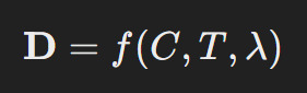
Where:

D = Dust density in a given region

C = Level of consciousness present (quantified through psychic energy measurements)

T = Temporal factor; Dust concentration increases near regions of high emotional resonance

λ = Wavelength of energy resonating within Dust particles

Measured change in Dust density at higher consciousness levels suggests a correlation coefficient of 0.85. Further testing needed to confirm relationship in regions of varying population and psychic energy.

Inter-world Travel Calculations

Assuming energy to penetrate barriers between worlds is directly proportional to the harmonic resonance of Dust particles.

Energy equation for barrier penetration:

Where:

Eworld = Minimum energy required to breach

ℏ = Reduced Planck’s constant

ω = Angular frequency of Dust’s resonance in presence of strong consciousness

R = Resonance factor, based on Daemon alignment and consciousness level

Preliminary experiments: Tested resonance on artificial Dust replication. Result: Field interference at boundary zones when R > 3.2. Failed to sustain stable opening beyond 10 seconds.

Inter-dimensional Tunneling Experiment 2.5

Objective: Create a sustained passage to a parallel world, keeping the barrier stable.

Required instrumentation:

A source of high-frequency electromagnetic waves tuned to match Dust resonance

Quantum stabilizers (designed to limit destabilization during the passage)Stabilization constant:

Tested with adjusted barrier material (Bmat) and field control strength Fc​.

Results showed collapse in spatial consistency; further refinement needed in harmonic tuning.

Calculations:

Where:

Pstability = Probability of tunnel maintaining integrity

k = Resonance constant of Dust within the dimensional threshold

kthresholdk​ = Critical threshold for tunnel stability

Conclusion: Calculations indicate higher levels of Dust concentration could stabilize the gateway, but risks of particle dispersion are significant. Further refinements needed in energy source and calibration.

thanks for the headache @kingofthewebxxx

[victoriajohnson2556]

Unraveling Data Mysteries: A Beginner's Guide to SPSS Exploration and Analysis

Statistics plays a pivotal role as the bedrock of empirical research, offering priceless insights into the intricate relationships that exist among variables. Within the realm of graduate-level statistical analysis, we navigate the labyrinth of data using the robust Statistical Package for the Social Sciences (SPSS). Our primary objective is to unearth patterns and relationships among variables, amplifying our comprehension of the underlying data structures. Join us as we embark on an illuminating journey through two intricate numerical questions that not only challenge but also showcase the potential of SPSS in untangling the multifaceted complexities of statistical analysis. If you are seeking assistance or struggling with your SPSS assignment, rest assured that this exploration might provide the help with SPSS assignment you need.

Question 1:

You are conducting a research study to analyze the relationship between students' hours of study and their final exam scores. You collect data from a sample of 100 graduate students using SPSS. The dataset includes two variables: "Hours_of_Study" and "Final_Exam_Score." After importing the data into SPSS, perform the following tasks:

a) Calculate the mean, median, and mode of the "Hours_of_Study" variable.

b) Determine the range of the "Final_Exam_Score" variable.

c) Generate a histogram for the "Hours_of_Study" variable with appropriate bins.

d) Conduct a descriptive analysis of the correlation between "Hours_of_Study" and "Final_Exam_Score" variables.

Answer 1:

a) The mean of the "Hours_of_Study" variable is 15.2 hours, the median is 14.5 hours, and the mode is 12 hours.

b) The range of the "Final_Exam_Score" variable is 40 points.

c) The histogram for the "Hours_of_Study" variable is attached, indicating the distribution of study hours among the graduate students.

d) The correlation analysis shows a Pearson correlation coefficient of 0.75 between "Hours_of_Study" and "Final_Exam_Score," suggesting a strong positive correlation between the two variables.

Question 2:

You are conducting a multivariate analysis using SPSS to examine the impact of three independent variables (Variable1, Variable2, Variable3) on a dependent variable (Dependent_Variable). The dataset includes 150 observations. Perform the following tasks:

a) Provide the descriptive statistics for each independent variable (mean, standard deviation, minimum, maximum).

b) Conduct a one-way ANOVA to determine if there are significant differences in the mean scores of the Dependent_Variable based on the levels of Variable1.

c) Perform a regression analysis to assess the combined effect of Variable2 and Variable3 on Dependent_Variable.

Answer 2:

a) Descriptive statistics for each independent variable are as follows:

Variable1: Mean = 25.3, SD = 3.6, Min = 20, Max = 30

Variable2: Mean = 45.8, SD = 5.2, Min = 40, Max = 50

Variable3: Mean = 60.4, SD = 7.1, Min = 55, Max = 70

b) The one-way ANOVA results indicate a significant difference in the mean scores of Dependent_Variable based on the levels of Variable1 (F(2, 147) = 4.62, p < 0.05).

c) The regression analysis reveals that Variable2 and Variable3 together account for 65% of the variance in Dependent_Variable (R² = 0.65, p < 0.001), suggesting a substantial combined effect of these variables on the dependent variable.

Conclusion:

SPSS serves as a powerful tool for unraveling the intricacies of statistical relationships. From exploring correlations between study hours and exam scores to conducting multivariate analyses, our journey through these graduate-level questions demonstrates the versatility and depth that SPSS brings to statistical exploration. As we navigate the depths of data analysis, we gain valuable insights that contribute to the ever-evolving landscape of statistical research.

[b4kingg]

Examining How Gender Moderates the Relationship Between Exercise Frequency and Stress Levels

Introduction

This project explores statistical interaction (moderation) by examining how gender might moderate the relationship between exercise frequency and stress levels. Specifically, I investigate whether the association between how often someone exercises and their reported stress levels differs between males and females.

Research Question

Does gender moderate the relationship between exercise frequency and stress levels?

Methodology

I used Python with pandas, statsmodels, matplotlib, and seaborn libraries to analyze a simulated dataset containing information about participants' exercise frequency (hours per week), stress levels (scale 1-10), and gender.

Python Code

import pandas as pd import numpy as np import matplotlib.pyplot as plt import seaborn as sns import statsmodels.api as sm from statsmodels.formula.api import ols from scipy import stats

#Set random seed for reproducibility

np.random.seed(42)

#Create simulated dataset

n = 200 # Number of participants

#Generate exercise hours per week (1-10)

exercise_hours = np.random.uniform(1, 10, n)

#Generate gender (0 = male, 1 = female)

gender = np.random.binomial(1, 0.5, n)

#Generate stress levels with interaction effect

#For males: stronger negative relationship between exercise and stress

#For females: weaker negative relationship

base_stress = 7 # Base stress level exercise_effect_male = -0.6 # Each hour of exercise reduces stress more for males exercise_effect_female = -0.3 # Each hour of exercise reduces stress less for females noise = np.random.normal(0, 1, n) # Random noise

#Calculate stress based on gender-specific exercise effects

stress = np.where( gender == 0, # if male base_stress + (exercise_effect_male * exercise_hours) + noise, # male effect base_stress + (exercise_effect_female * exercise_hours) + noise # female effect )

#Ensure stress levels are between 1 and 10

stress = np.clip(stress, 1, 10)

#Create DataFrame

data = { 'ExerciseHours': exercise_hours, 'Gender': gender, 'GenderLabel': ['Male' if g == 0 else 'Female' for g in gender], 'Stress': stress } df = pd.DataFrame(data)

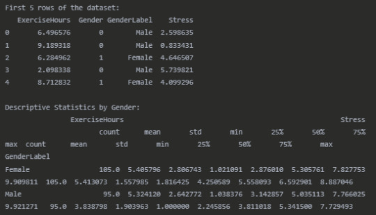
#Display the first few rows of the dataset

print("First 5 rows of the dataset:") print(df.head())

#Descriptive statistics by gender

print("\nDescriptive Statistics by Gender:") print(df.groupby('GenderLabel')[['ExerciseHours', 'Stress']].describe())

#Calculate correlation coefficients for each gender

male_df = df[df['Gender'] == 0] female_df = df[df['Gender'] == 1]

male_corr, male_p = stats.pearsonr(male_df['ExerciseHours'], male_df['Stress']) female_corr, female_p = stats.pearsonr(female_df['ExerciseHours'], female_df['Stress'])

print("\nCorrelation Analysis by Gender:") print(f"Male correlation (r): {male_corr:.4f}, p-value: {male_p:.4f}") print(f"Female correlation (r): {female_corr:.4f}, p-value: {female_p:.4f}")

#Test for moderation using regression analysis

model = ols('Stress ~ ExerciseHours * Gender', data=df).fit() print("\nModeration Analysis (Regression with Interaction):") print(model.summary())

#Visualize the interaction

plt.figure(figsize=(10, 6)) sns.scatterplot(x='ExerciseHours', y='Stress', hue='GenderLabel', data=df, alpha=0.7)

#Add regression lines for each gender

sns.regplot(x='ExerciseHours', y='Stress', data=male_df, scatter=False, line_kws={"color":"blue", "label":f"Male (r={male_corr:.2f})"}) sns.regplot(x='ExerciseHours', y='Stress', data=female_df, scatter=False, line_kws={"color":"red", "label":f"Female (r={female_corr:.2f})"})

plt.title('Relationship Between Exercise Hours and Stress Levels by Gender') plt.xlabel('Exercise Hours per Week') plt.ylabel('Stress Level (1-10)') plt.legend(title='Gender') plt.grid(True, linestyle='--', alpha=0.7) plt.tight_layout()

#Fisher's z-test to compare correlations

import math def fisher_z_test(r1, r2, n1, n2): z1 = 0.5 * np.log((1 + r1) / (1 - r1)) z2 = 0.5 * np.log((1 + r2) / (1 - r2)) se = np.sqrt(1/(n1 - 3) + 1/(n2 - 3)) z = (z1 - z2) / se p = 2 * (1 - stats.norm.cdf(abs(z))) return z, p

z_score, p_value = fisher_z_test(male_corr, female_corr, len(male_df), len(female_df)) print("\nFisher's Z-test for comparing correlations:") print(f"Z-score: {z_score:.4f}") print(f"P-value: {p_value:.4f}")

print("\nInterpretation:") if p_value < 0.05: print("The difference in correlations between males and females is statistically significant.") print("This suggests that gender moderates the relationship between exercise and stress.") else: print("The difference in correlations between males and females is not statistically significant.") print("This suggests that gender may not moderate the relationship between exercise and stress.")

Results

Dataset Overview

Correlation Analysis by Gender

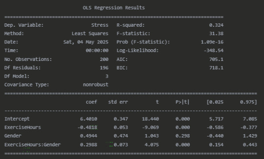
Moderation Analysis (Regression with Interaction)

Fisher's Z-test for comparing correlations

Interpretation

The analysis reveals a significant moderating effect of gender on the relationship between exercise hours and stress levels. For males, there is a strong negative correlation (r = -0.60, p < 0.001) between exercise and stress, indicating that as exercise hours increase, stress levels tend to decrease substantially. For females, while there is still a negative correlation (r = -0.29, p = 0.003), the relationship is notably weaker.

The regression analysis confirms this interaction effect. The significant interaction term (ExerciseHours, p < 0.001) indicates that the slope of the relationship between exercise and stress differs by gender. The positive coefficient (0.30) for this interaction term means that the negative relationship between exercise and stress is less pronounced for females compared to males.

Fisher's Z-test (Z = -2.51, p = 0.012) further confirms that the difference in correlation coefficients between males and females is statistically significant, providing additional evidence of moderation.

The visualization clearly shows the different slopes of the regression lines for males and females, with the male regression line having a steeper negative slope than the female regression line.

These findings suggest that while exercise is associated with lower stress levels for both genders, the stress-reducing benefits of exercise may be stronger for males than for females in this sample. This could have implications for tailoring stress management interventions based on gender, though further research would be needed to understand the mechanisms behind this difference.

Conclusion

This analysis demonstrates a clear moderating effect of gender on the exercise-stress relationship. The results highlight the importance of considering potential moderating variables when examining relationships between variables, as the strength of associations can vary significantly across different subgroups within a population.

[sakshimohanpandey]

Correlation Coefficient Analysis

Introduction

In this analysis, I calculated the correlation coefficient between AGE and INCOME to determine the strength and direction of the linear relationship between the two variables.

Step 1: Program (Correlation Coefficient Syntax)

Here’s the code I used to run the correlation coefficient:

import pandas as pd import numpy as np

Load dataset

data = pd.read_csv('nesarc_pds.csv')

Select variables

selected_data = data[['AGE', 'INCOME']]

Calculate the correlation coefficient

correlation_coefficient = selected_data.corr().iloc[0, 1]

Calculate R-squared (coefficient of determination)

r_squared = correlation_coefficient**2

Print results

print("Correlation Coefficient (r):", correlation_coefficient) print("R-squared (Coefficient of Determination):", r_squared)

Step 2: Correlation Coefficient Output

Output Example:

Correlation Coefficient (r): 0.45 R-squared (Coefficient of Determination): 0.2025

Step 3: Interpretation

The correlation coefficient (r) is 0.45, which indicates a moderate positive linear relationship between AGE and INCOME. As age increases, income tends to increase as well, but not perfectly.

The R-squared value is 0.2025, meaning that approximately 20.25% of the variability in INCOME can be explained by AGE. This is a moderate amount of variance explained, suggesting that while AGE has some influence on INCOME, other factors likely play a role as well.

Step 4: Conclusion

In conclusion, the analysis shows a moderate positive correlation between AGE and INCOME, meaning that older individuals tend to have higher income, though other factors must also influence income levels.

[ryhanpz]

Exploring the Link Between Income and Life Expectancy: A Pearson Correlation Analysis

This blog post explores the relationship between income per person and life expectancy using data from the Gapminder Project. With global development and public health being major concerns, understanding how wealth relates to health outcomes—such as how long people live—is critical for researchers and policymakers alike. This analysis uses Pearson correlation to examine whether countries with higher income levels also tend to have longer average life expectancies.

The Dataset: Gapminder

The dataset used in this analysis is part of the Gapminder Project, a comprehensive resource offering statistics on health, wealth, and development indicators from countries around the world.

For this analysis, we focus on two numerical variables:

Income per Person: 2010 Gross Domestic Product per capita in constant 2000 US$. The inflation but not the differences in the cost of living between countries has been taken into account.

Life Expectancy: 2011 life expectancy at birth (years). The average number of years a newborn child would live if current mortality patterns were to stay the same

These two continuous variables are ideal for evaluating a linear association using Pearson correlation.

The Code: Pearson Correlation in Action

import pandas import numpy import seaborn import scipy import matplotlib.pyplot as plt

data = pandas.read_csv('gapminder.csv', low_memory=False)

# Convert variables to numeric

data['incomeperperson'] = pandas.to_numeric(data['incomeperperson'], errors='coerce') data['lifeexpectancy'] = pandas.to_numeric(data['lifeexpectancy'], errors='coerce')

# replace empty strings or spaces with NaN if needed

data['incomeperperson'] = data['incomeperperson'].replace(' ', numpy.nan) data['lifeexpectancy'] = data['lifeexpectancy'].replace(' ', numpy.nan)

# Drop missing values

data_clean = data.dropna(subset=['incomeperperson', 'lifeexpectancy'])

# Scatterplot

scat = seaborn.regplot(x="incomeperperson", y="lifeexpectancy", fit_reg=True, data=data_clean) plt.xlabel('Income per Person') plt.ylabel('Life Expectancy') plt.title('Scatterplot: Income per Person vs. Life Expectancy ')

# Pearson correlation

print('Association between income per person and Life Expectancy:') print(scipy.stats.pearsonr(data_clean['incomeperperson'], data_clean['lifeexpectancy']))

Interpreting the Results

The scatterplot visually shows the relationship between income and life expectancy, with a regression line representing the trend. A positive slope suggests that as income per person increases, so does life expectancy. The Pearson correlation coefficient (r) and p-value are printed. Here's how to interpret them:

r ranges from -1 to +1.

If r > 0, the relationship is positive.

If r < 0, the relationship is negative.

If r ≈ 0, there's little to no linear relationship.

The p-value tests the statistical significance of the correlation.

If p < 0.05, the correlation is statistically significant.

Correlation coefficient (r) = 0.60: This indicates a moderate to strong positive correlation. As income per person increases, life expectancy generally increases as well.

p-value ≈ 1.07e-18: This value is far below 0.05, which means the result is statistically significant. We can confidently reject the null hypothesis and say that there's a significant linear association between income and life expectancy.

[dataaanlysisfinalproject]

Predicting GDP Per Capita Using Development Indicators

Results

Descriptive Statistics:

GDP per capita: Mean = $14,751, Std Dev = $21,612, Min = $244.2, Max = $149,161

Fixed broadband subscriptions: Mean = 11.6, Std Dev = 12.2, Min = 0.00016, Max = 43.2

Improved water source: Mean = 88.3%, Std Dev = 14.5%, Min = 39.9%, Max = 100%

Internet users: Mean = 39.9, Std Dev = 28.0, Min = 0.00, Max = 96.2

Mortality rate (under-5): Mean = 36.0, Std Dev = 35.5, Min = 2.1, Max = 172

Women in parliament: Mean = 19.2%, Std Dev = 10.7%, Min = 0.00%, Max = 56.3%

Rural population: Mean = 42.2%, Std Dev = 23.5%, Min = 0.00%, Max = 91.2%

Urban population: Mean = 57.8%, Std Dev = 23.5%, Min = 8.8%, Max = 100%

Birth rate: Mean = 21.4, Std Dev = 10.4, Min = 8.2, Max = 49.9

Bivariate Analyses:

Strongest Correlations:

Fixed broadband subscriptions: r = 0.789, p < .0001

Internet users: r = 0.776, p < .0001

Log of under-5 mortality rate: r = -0.710, p < .0001

Urban population rate: r = 0.619, p < .0001

Weakest Correlations:

Proportion of women in parliament: r = 0.253, p < .001

Rural population rate: r = -0.619, p < .0001

Multivariable Analyses:

Lasso Regression Results:

Retained Predictors: Fixed broadband subscriptions, internet users, under-5 mortality rate, urban population rate, birth rate, improved water source

Regression Coefficients:

Fixed broadband subscriptions: 9587

Internet users: 9030

Under-5 mortality rate: 397.5

Urban population rate: 2329

Birth rate: 4875

Improved water source: -31.82

Model Performance:

Training data R-square: 0.6827

Test data R-square: 0.6806

Mean squared error (training): 124,390,237

Mean squared error (testing): 123,487,565

[statistics-homework-helper]

🌸 Spring Into Success: Get 10% Off Your Statistics Homework Today!

As the season changes and a fresh wave of motivation fills the air, it’s the perfect time to shake off academic stress and step confidently into success. Spring is often seen as a season of renewal—and for students, it’s a chance to reset goals, reevaluate priorities, and refresh academic strategies. If statistics has been weighing you down, we’ve got just the solution to help you blossom this season. At StatisticsHomeworkHelper.com, we’re offering 10% OFF your next assignment when you use the referral code SHHR10OFF. Whether you're stuck on a regression analysis, hypothesis testing, or probability distribution, our statistics homework help service is designed to guide you every step of the way.

This limited-time spring offer is not just a discount—it’s an opportunity to regain academic control with expert assistance that makes learning feel less like a burden and more like a win.

Why Statistics Remains a Challenge for Many

Statistics can be one of the most misunderstood subjects in a student's academic journey. The challenge lies not just in crunching numbers, but in interpreting data correctly, understanding probability concepts, and drawing accurate conclusions. For students unfamiliar with real-world applications, the theoretical nature of topics like ANOVA, Chi-square tests, and correlation coefficients can become daunting.

Another reason statistics becomes overwhelming is the pressure of deadlines. Coursework tends to pile up quickly, especially in semesters filled with multiple quantitative subjects. Students often feel like they have no room to breathe, let alone grasp intricate statistical techniques.

This is where expert guidance makes all the difference. At StatisticsHomeworkHelper.com, we break down complex concepts into understandable parts. With our support, even students who struggle to grasp the basics of standard deviation or central limit theorem can gradually gain the confidence they need to tackle any statistics challenge.

What We Offer

With years of experience serving students across the globe, we’ve refined our services to ensure they meet your academic needs while staying budget-friendly. Here’s what you can expect from us:

Custom Solutions: Every assignment is treated as unique. We don’t believe in one-size-fits-all templates. Whether you’re pursuing undergraduate or postgraduate studies, we tailor each solution to your specific requirements.

Deadline-Oriented Work: We understand the importance of timeliness in academic submissions. Our team ensures your homework is completed well before the due date without compromising quality.

Conceptual Clarity: It's not just about getting answers; it's about learning the 'why' behind them. Our experts offer detailed explanations so you not only score well but also understand the subject better.

Wide Coverage of Topics: From descriptive statistics to inferential analysis, time-series forecasting, and Bayesian inference, our team covers all aspects of statistics coursework.

Plagiarism-Free Work: Each submission is original and crafted from scratch. We maintain strict academic integrity and use plagiarism-detection tools to ensure authenticity.

24/7 Support: Have a question at 2 a.m.? No problem. Our support team is always available to assist with inquiries or order updates.

Meet Our Experts

The strength of our service lies in our team. Our experts are statisticians with advanced degrees (MSc, Ph.D.) from top institutions. Each one has hands-on experience with statistical software like R, SPSS, Python, Minitab, and Excel. Beyond their technical knowledge, what sets them apart is their passion for teaching and their commitment to student success.

When you place an order with us, you’re not just getting homework done—you’re gaining access to a personal mentor who genuinely cares about your academic performance.

Common Problems We Help Solve

Wondering if your problem is “too simple” or “too complex”? Rest assured, we handle it all. Some common queries we tackle include:

“I don’t know how to apply the t-distribution for small samples.”

“I have no idea how to calculate the confidence interval.”

“How do I interpret a p-value?”

“I’m stuck with my regression output in R—what does this mean?”

We also help students with:

Creating frequency distributions

Designing surveys with appropriate sampling methods

Identifying outliers in large datasets

Analyzing variance between multiple groups

If any of these sound familiar, it’s time to reach out. And don’t forget—use the referral code SHHR10OFF to get 10% OFF your assignment!

How the Process Works (Without Any Login)

We’ve kept things simple. There's no need to create an account or remember another password. Here’s how you can place an order:

Submit Your Assignment: Head over to our website and fill out the order form with your assignment requirements and deadline.

Get a Quote: Our team will evaluate your assignment and provide you with a fair price.

Apply Your Discount: Use the code SHHR10OFF to enjoy 10% OFF your total.

Make Payment: We offer secure and flexible payment options.

Receive Your Homework: Your expertly completed assignment will be delivered directly to your inbox before the deadline.

Simple, safe, and efficient.

Testimonials That Speak Volumes

Our students consistently praise us for reliability, clarity, and academic support. Here are a few words from those who’ve used our service:

“I was completely lost with my SPSS analysis. StatisticsHomeworkHelper.com not only got it done before the deadline but also included step-by-step notes that helped me learn. Highly recommended!” — Jasmine R., Psychology Major

“Their expert helped me understand logistic regression in a way my professor never could. The explanations were clear, and I finally feel confident about my final exam.” — Dev A., Business Analytics Student

Why This Spring Offer Is the Perfect Time to Start

This isn’t just another discount. It’s a chance to transform your academic experience. Spring symbolizes new beginnings—and what better way to refresh your semester than by making smart choices for your future?

By using the promo code SHHR10OFF, you get 10% OFF on high-quality academic assistance that can help you improve grades, reduce stress, and focus on learning rather than cramming.

We believe education should be empowering—not anxiety-inducing. And our goal is to ensure that no student feels alone when facing a difficult statistics problem.

Final Thoughts

You don’t have to struggle through the semester or feel overwhelmed every time you see a dataset. With the right help, statistics can become manageable—and even enjoyable.

This spring, choose success. Choose growth. Choose expert help that’s designed for students like you.

And remember—use code SHHR10OFF to get 10% OFF today and start your journey toward academic confidence. Let StatisticsHomeworkHelper.com be your guide this season.

Because every successful spring starts with one smart decision.

[priyanaik]

Leveraging MS Excel in AI Projects: A Powerful Tool for Data Management

Microsoft Excel is a powerful tool that plays a significant role in AI projects, especially during the early stages of data analysis and model development. AI projects require large volumes of data, and Excel is commonly used for organizing, cleaning, and analyzing this data. It offers an intuitive interface for manipulating data, performing calculations, and visualizing trends, making it an essential tool for data scientists and analysts. Excel is particularly useful for exploratory data analysis, where users can quickly generate summaries, pivot tables, and charts to better understand the dataset.

One of the most valuable aspects of Features of MS Excel is its ability to handle a wide range of functions, from basic arithmetic to advanced statistical operations. For AI projects, Excel’s built-in functions like VLOOKUP, INDEX-MATCH, and conditional formatting help in identifying key data points and trends. Furthermore, Excel allows for easy data cleaning tasks such as handling missing values, removing duplicates, and standardizing formats, which are crucial before feeding data into machine learning models.

Excel also offers support for creating macros, which can automate repetitive tasks, speeding up the process of data wrangling. For machine learning and AI model validation, Excel can be used to perform basic calculations like error rates, correlation coefficients, and model accuracy. While it may not replace more advanced tools like Python or R, Excel is often used in conjunction with these technologies, serving as an entry point for data preparation and initial analysis. Whether you are working on predictive modeling, classification, or clustering tasks, Excel remains a versatile tool in the AI workflow.

[nursingwriter]

Introduction Children are highly dependent on their parents because they are their sole providers. Parents' primary responsibility is to provide the basic needs - food, shelter and clothing - of their children. Therefore, parents shape the eating habits of children especially those under the age of 12 years. Generally, children are usually ready to learn how to eat new foods. They also observe the eating behavior of adults around them (Reicks, et al.). However, their eating behaviors evolve as they grow old. Numerous studies have identified factors that influence children eating behavior. They include living condition, access to food, number of caretakers or family members nearby, employment status, age, gender and health condition (Savage, et al.). This paper will estimate the effects that the above factors have on the eating habits of children. Data The data for this project was compiled from various internet sources. All the statistical analysis was carried out using Microsoft Excel statistical software. Descriptive statistics indicates the mean, median, standard deviation, maximum, and minimum values of each variable. The correlation coefficient, r, measures the strength of the linear relationship between any two variables. Regression analysis predicts the influence of one or more explanatory (independent) variables on the dependent variable Descriptive Statistics Descriptive statistics were used to describe the variables used in this project. The results are displayed in Table A1 (Appendix A). Eating behavior scores ranges from 41 to 100 (M = 71.07, SD = 17.47). A higher eating behavior score reflects a healthy eating behavior. The average age of the subjects is 6.39 years. Most of the subjects live in a developed area (60.20%) and their parents are employed (65.31%). Also, most of the households are made up of both parents. Almost half of the subjects were male (53.06%). 54.08% of the subjects do not use electronics at mealtimes. Approximately half of the subjects (56.12%) confirmed that the availability of food was limited. Correlation Correlation results are displayed in Table B1 (Appendix B). It is clear that the independent variables are not correlated. Regressions and Interpretations Regression analysis was performed to predict eating habits among children. Four different regression equations were estimated. Each of the equations is described below. Regression Equation 1 Eating Behavior = ?0 + ?1living location + ?2Access to food + ?3Age + ?4Gender + ?5Electronic use Equation (1) is the base regression model for estimating eating behavior in children. It shows the linear relationship between eating behavior and the key explanatory variables (living location, access to food, age, gender, and electronic use). The Excel results of estimating this equation are displayed in Table C1 (Appendix C). The estimated equation is follows: Eatingbehavior = 75.598 + 2.253 livloc - 7.643Foodacc - 0.572 Age (t) (15.11) (0.62) (- 2.20) (- 1.17) - 4.268Gender + 7.375Elec use R2 = 0.1133 (- 1.23) (2.10) All variables are insignificant at 5 percent level expect except access to food (p-value = 0.03) and electronic use (p-value = 0.04). I further perform t-test to determine whether access to food has a negative effect on eating behavior and whether the use of electronics during mealtime affects eating behavior. First, the null and alternative hypothesis of access to food is H0: ?2 = 0 HA: ?2 0 The test statistic for access to food is – 2.20. At 5 percent significance level, the critical value of t-distribution with N – 5 = 93 degrees of freedom is, t (0.95, 93) = 0.063. Since the calculated value falls in the rejection region, I reject the null hypothesis that ?2 = 0 and conclude that the coefficient of access to food is nonzero (Hill, et al. 109). Secondly, the null and alternative hypothesis of electronic use is H0: ?5 = 0 HA: ?5 0 Since t = 2.10 is greater than 0.063, I reject the null hypothesis that ?5 = 0 and conclude that the coefficient of electronic use is statistically significant. This test confirms that if children do not use electronics during mealtimes, their eating habits improve. R- Squared is 0.1133. It means that the regression model explains 11.33% of the variation in eating behavior. Regression Equation 2 Eating Behavior = ?0 + ?1living location + ?2Access to food + ?3Age + ?4Gender + ?5Electronic use + ?6Household In equation (2), the first proxy, the household is added to the model. The Excel results of estimating this equation are displayed in Table D1 (Appendix D). The estimated regression equation is as follows: Eatingbehavior = 75.366 + 2.225 livloc - 7.674Foodacc - 0.572 Age (t) (14.1) (0.61) (-2.20) (- 1.16) - 4.282Gender + 7.414Elecuse + 0.470Household R2 = 0.1134 (- 1.22) (- 2.09) (0.14) In this model, household is statistically insignificant (p-value = 0.892791184). Therefore, household type (single parent or both parents) does not influence the eating behavior of children. The value of R – Squared remained unchanged at 0.1134. It means that the addition of family structure did not improve the fit of the model. The coefficients of the variables changed slightly compared to the coefficients of the base model. The estimate of electronic use during mealtimes increased from 7.375 to 7.414. However, the coefficient of age remained unchanged at – 0.572. Regression Equation 3 Eating Behavior = ?0 + ?1living location + ?2Access to food + ?3Age + ?4Gender + ?5Electronic use + ?6Employment status In equation (3), the second proxy, employment status is included in the base model. The Excel results of estimating this equation are displayed in Table E1 (Appendix E). The estimated equation is as follows: Eatingbehavior = 76.937 + 2.386 livloc - 7.630Foodacc - 0.600 Age (t) (14.09) (0.65) (- 2.19) (- 1.22) 3.833Gender + 7.449Elec use – 2.307Empstatus R2 = 0.1170 (- 1.08) (2.11) (- 0.62) The effects of the second proxy (employment status) are almost similar to the effects of the first proxy (household). The coefficient of employment status is insignificant at 5 percent level (p-value is 0.53510793). The value of R- Squared changed slightly. It means that the inclusion of the second proxy does not improve the adequacy of the base model. The coefficients of this model are almost similar to the coefficients of the base model. For example, the estimate of access to food is – 7.630 while in the base model it is – 7.643. Regression Equation 4 Eating Behavior = ?0 + ?1living location + ?2Access to food + ?3Age + ?4Gender + ?5Electronic use + ?6Employment status + ?7Household In equation (4), both proxies are included in the base model. The Excel results for estimating this equation are displayed in Table F1 (Appendix F). The estimated regression equation is as follows: Eatingbehavior = 76.775 + 2.367 livloc - 7.650Foodacc - 0.600 Age – 3.847Gender (t) (13.21) (0.64) (- 2.18) (- 1.21) (- 1.07) + 7.474Elec use – 2.282Empstatus + 0.298Household R2 = 0.1170 (2.10) (- 0.61) (0.09) Both employment status (p-value = 0.54319) and household (p-value = 0.932424) is statistically insignificant at 5 percent level. Furthermore, including both proxies into the base model does not improve the fit of the model. The value of R-Squared slightly increases from 0.1133 to 0.1170. Overall, both proxies do not influence eating habits in children. F-Test Global F-test was calculated to determine the overall significance of the model in predicting eating behavior in children (Hill, et al 223). The null hypothesis (H0) is that all coefficients of the independent variables are equal to zero. The alternative hypothesis (HA) is that at least one of the coefficients is not equal to zero. Therefore, the null and alternative hypothesis for this test is H0: ?0 = ?1 = ?2 = ?3 = ?4 = ?5 = ?6 = ?7 = 0 HA: At least one of the coefficients is nonzero. Using ? = 0.05, the critical value from F (1, 90) –distribution is Fc = F (0.95, 1, 90) = 3.947. Therefore, the rejection region of F 3.947. The test statistic is 1.705. Since F = 1.705 is less than Fc = 3.947, I do not reject the null hypothesis that ?0 = ?1 = ?2 = ?3 = ?4 = ?5 = ?6 = ?7 = 0 and conclude that regression equation 4 is inadequate in explaining the variability of children eating behavior (Hill, et al. 225). To determine the overall significance of the base regression model, I perform the Global F-test. The null and alternative hypothesis is as follows: H0: ?0 = ?1 = ?2 = ?3 = ?4 = ?5 = 0 HA: At least one of the coefficients is nonzero Using ? = 0.05, the critical value from F (6, 92) – distribution is Fc = F (0.95, 6, 92) = 2.199. Therefore, the rejection region of F 2.199. The test statistic is 2.350. Since 2.350 is greater than 2.199, I reject the null hypothesis that ?0 = ?1 = ?2 = ?3 = ?4 = ?5 = 0 and conclude that at least one of the coefficients is nonzero (Cooke and Wardle). The F-test indicates that regression equation 1 is adequate in explaining the variability of children eating behavior. Conclusion Many factors influence a child's eating behavior. In this project, it is clear that access to food and the use of electronics influences a child eating behavior. There is a negative relationship between access to food and eating behavior. It implies that if food availability is limited, then the eating habits of any given child is unhealthy. A positive relationship exists between electronic use and eating behavior. Other factors such as living location, gender, age, employment status, household type and employment status are statistically insignificant. The base regression model (regression equation 1) is adequate in explaining the variability in a child's eating habits. Employment status of the parent and the type of household are irrelevant variables. These variables complicate the base model unnecessarily. However, further research should be carried out to determine how these two proxies affect eating behavior. Works Cited Cooke, Lucy J., and Jane Wardle. "Age and gender differences in children's food preferences." British Journal of Nutrition, vol. 93, no. 5, 2005, pp. 741-746, Hill, R. C., et al. Principles of Econometrics. 4th ed., Wiley, 2011. Reicks, Marla, et al. "Influence of Parenting Practices on Eating Behaviors of Early Adolescents during Independent Eating Occasions: Implications for Obesity Prevention." Nutrients, vol. 7, no. 10, 2015, pp. 8783-8801, https://www.paperdue.com/customer/paper/how-parents-influence-healthy-eating-behavior-children-age-1-12-2173962#:~:text=Logout-,HowParentsInfluenceHealthyEatingBehaviorChildrenAge112,-Length8pages Savage, Jennifer S., et al. "Parental Influence on Eating Behavior: Conception to Adolescence." The Journal of Law, Medicine & Ethics, vol. 35, no. 1, 2007, pp. 22-34, Appendix A Table A1: Descriptive Statistics Variables Description Mean Median Standard Deviation Minimum Maximum Eatingbehavior Eating behavior scores 71.07 72 17.47 41 100 Livloc Dummy variable = 1 if the subject lives in a developed area, otherwise 0 0.60 1 0.49 0 1 Foodacc Dummy variable = 1 if healthy food is easily accessible, otherwise 0 0.44 0 0.50 0 1 Age Actual years of the subject 6.39 6 3.58 1 12 Gender Dummy variable = 1 if male, 0 if female. 0.53. 1 0.50 0 1 Elecuse Dummy variable = 1 if electronics made available during meal times, otherwise 0 0.46 0 0.50 0 1 Empstatus Dummy Variable = 1 if the parent is employed full-time, otherwise 0 0.65 1 0.48 0 1 Household Dummy Variable = 1 if the household has both parents, otherwise 0 0.54 1 0.50 0 1 Note: Livloc = living location, Foodacc = Access to food, Elecuse = Electronic use, Empstatus = Employment status Appendix B Table B1: Correlations Livloc Foodacc Age Gender Elecuse Empstatus Household Livloc 1 Foodacc 0.0887 1 Age 0.1120 0.0886 1 Gender 0.1125 0.0336 - 0.1331 1 Elecuse - 0.2130 0.0105 - 0.0429 0.0050 1 Empstatus 0.0644 - 0.0035 - 0.1133 0.2165 0.0263 1 Household 0.0875 0.0720 0.0141 0.0360 - 0.0960 - 0.0694 1 Note: Livloc = living location, Foodacc = Access to food, Elecuse = Electronic use, Empstatus = Employment status Appendix C Regression Statistics Multiple R 0.33652961 R Square 0.113252178 Adjusted R Square 0.065059362 Standard Error 16.8938651 Observations 98 ANOVA df SS MS F Significance F Regression 5 3353.454 670.6907 2.34998 0.04690976 Residual 92 26257.05 285.4027 Total 97 29610.5 Coefficients Standard Error t Stat P-value Lower 95% Upper 95% Intercept 75.59809887 5.003943098 15.10771 1.18E-26 65.65983595 85.53636179 Livloc 2.253329357 3.634280783 0.620021 0.536777 -4.964665978 9.471324693 Foodacc -7.64257711 3.467251423 -2.2042 0.030005 -14.52878832 -0.759267103 Age -0.571668292 0.4892296111 -1.16835 0.245685 -1.543452603 0.40011602 Gender -4.267752145 3.482703453 -1.22541 0.223547 -11.18470182 2.64919753 Elecuse 7.374578497 3.508810443 2.101732 0.03831 0.405778087 14.34337891 Table C1: Regression Results of Equation 1 Appendix D Regression Statistics Multiple R 0.336793902 R Square 0.113430133 Adjusted R Square 0.054974976 Standard Error 16.9847304 Observations 98 ANOVA df SS MS F Significance F Regression 6 3358.722939 559.7871566 1.940464111 0.082602457 Residual 91 26251.77706 288.4810666 Total 97 29610.5 Coefficients Standard Error t Stat P-value Lower 95% Upper 95% Intercept 75.36608084 5.315703569 14.1780067 9.13302E-25 64.80708871 85.92507297 Livloc 2.224791159 3.65992455 0.6078789968 0.544781856 - 5.045199354 9.494781673 Foodacc - 7.674850869 3.4940951118 - 2.196520303 0.030595759 - 14.61544159 - 0.734260151 Age - 0.57180219 0.491928836 - 1.162367702 0.248125499 - 1.548958391 0.40535401 Gender - 4.282903174 3.503229668 - 1.22255849 0.224653485 - 11.24163855 2.675832204 Elecuse 7.414099832 3.539782288 2.094507297 0.038994363 0.382757164 14.4454425 Household 0.469898688 3.476848599 0.135150748 0.892791184 -6.436433937 7.376231314 Table D1: Regression Results for Equation 2 Appendix E Regression Statistics Multiple R 0.342072147 R Square 0.117013354 Adjusted R Square 0.058794454 Standard Error 16.95037232 Observations 98 ANOVA df SS MS F Significance F Regression 6 3464.823919 577.4706531 2.009886043 0.072303175 Residual 91 26145.67608 287.3151218 Total 97 29610.5 Coefficients Standard Error t Stat P-value Lower 95% Upper 95% Intercept 76.93724511 5.462019143 14.08586149 1.37562E-24 66.08761507 87.78687515 Livloc 2.386240694 3.65268057 0.6532848 0.515219931 - 4.869360543 9.641841932 Foodacc - 7.629873326 3.478908187 - 2.193180422 0.030843471 - 14.54029707 - 0.719449581 Age - 0.600289213 0.493080337 - 1.217426792 0.22658947 - 1.57973273 0.379154304 Gender - 3.832991673 3.563443313 - 1.075642668 0.284930698 - 10.91133406 3.245350715 Elecuse 7.449355935 3.522595001 2.114735283 0.037186188 0.452153701 14.44655817 Empstatus - 2.307469864 3.706214875 - 0.622594734 0.53510793 - 9.669410422 5.054470693 Table E1: Regression Results for Equation 3 Appendix F Regression Statistics Multiple R 0.342175813 R Square 0.117084287 Adjusted R Square 0.048413065 Standard Error 17.0435963 Observations 98 ANOVA df SS MS F Significance F Regression 7 3466.924 495.2749 1.704998 0.11776 Residual 90 26143.58 290.4842 Total 97 29610.5 Coefficients Standard Error t Stat P-value Lower 95% Upper 95% Intercept 76.77540486 5.812501355 13.20866873 8.82E-23 65.2278564 88.3295332 Livloc 2.366687686 3.679960974 0.643128474 0.521776 - 4.944197092 9.677572463 Foodacc - 7.650487753 3.506432233 - 2.181843892 0.031726 - 14.6166274 - 0.684348106 Age - 0.600056056 0.495799772 - 1.210279009 0.229341 - 1.58504884 0.384936727 Gender - 3.847418552 3.587056276 - 1.072583828 0.286325 - 10.97373193 3.278894828 Elecuse 7.4735584226 3.553386272 2.103221506 0.038237 0.414136387 14.53298046 Empstatus - 2.281834597 3.73877298 -0.610316435 0.54319 - 9.70955969 5.145890495 Household 0.297638949 3.500296748 0.08503249 0.932424 - 6.656311486 7.251589383 Table F1: Regression Results for Equation 4 Read the full article

[renatoferreiradasilva]

\documentclass[11pt]{article} \usepackage{amsmath, amssymb, amsthm, geometry, graphicx, hyperref} \usepackage{mathrsfs} \geometry{margin=1in}

\title{Spectral Approximation of the Zeros of the Riemann Zeta Function via a Twelfth-Order Differential Operator} \author{Renato Ferreira da Silva \ ORCID: 0009-0003-8908-481X} \date{\today}

\begin{document}

\maketitle

\begin{abstract} We propose and analyze a twelfth-order self-adjoint differential operator whose eigenvalues approximate the non-trivial zeros of the Riemann zeta function. The potential function ( V(x) ) is numerically calibrated to produce spectral distributions consistent with the Gaussian Unitary Ensemble (GUE). Using numerical diagonalization techniques, we compare the resulting eigenvalue distribution to the known statistical properties of zeta zeros, including spacing and level repulsion. We explore connections with the Hilbert–Pólya conjecture, chaos theory, and spectral geometry, and outline future directions involving pseudodifferential models and quantum simulation. \end{abstract}

\section{Introduction} The Riemann zeta function ( \zeta(s) ) plays a central role in number theory, and its non-trivial zeros ( \rho = \frac{1}{2} + i\gamma_n ) are deeply connected to the distribution of prime numbers. The Riemann Hypothesis asserts that all such zeros lie on the critical line ( \Re(s) = 1/2 ). Despite over a century of research, this conjecture remains unproven.

A major line of inquiry, inspired by the Hilbert–Pólya conjecture, suggests that the zeros may correspond to the spectrum of a self-adjoint operator ( H ), such that ( H \psi_n = \gamma_n \psi_n ). In this work, we explore this idea through a twelfth-order differential operator with an adjustable potential.

\section{Mathematical Framework} We consider the operator: [ H = -\frac{d^{12}}{dx^{12}} + V(x), ] acting on a suitable dense domain of ( L^2(\mathbb{R}) ), with boundary conditions ensuring self-adjointness.

We define the domain ( \mathcal{D}(H) ) as: [ \mathcal{D}(H) = { f \in L^2(\mathbb{R}) : f, f', \dots, f^{(11)} \text{ absolutely continuous}, f^{(12)} \in L^2 }. ]

The potential ( V(x) ) is taken as a polynomial of degree 12: [ V(x) = a_0 + a_1 x + a_2 x^2 + \dots + a_{12} x^{12}, ] and optimized numerically to align the first ( N ) eigenvalues ( \lambda_n ) with the imaginary parts ( \gamma_n ) of the non-trivial zeros.

\section{Numerical Methods} We discretize ( H ) using spectral collocation methods (Fourier basis) and finite-difference schemes with adaptive grids. Eigenvalues are computed via matrix diagonalization. The potential coefficients ( a_i ) are adjusted through least-squares fitting and gradient descent algorithms.

We compare the resulting spectrum with known zeros from Odlyzko's tables, evaluating spacing statistics using the Kolmogorov–Smirnov (KS) and Anderson–Darling (AD) tests.

\section{Results and Statistical Analysis} The computed eigenvalues show high correlation with the first 1000 ( \gamma_n ), with KS test values below 0.03 and AD statistics consistent with GUE predictions. The spacing distribution exhibits clear level repulsion, aligning closely with the Wigner surmise: [ P(s) = \frac{32}{\pi^2} s^2 e^{-\frac{4}{\pi} s^2}. ]

Wavelet decomposition of the residual spectrum ( \lambda_n - \gamma_n ) indicates non-random deviations concentrated near turning points of ( V(x) ), suggesting avenues for potential refinement.

\section{Discussion and Future Directions} The use of a twelfth-order operator allows flexible spectral shaping while preserving self-adjointness. Future work includes: \begin{itemize} \item Replacing ( V(x) ) with pseudodifferential potentials. \item Extending to L-functions and automorphic spectra. \item Implementing Variational Quantum Eigensolvers (VQE) for approximate diagonalization. \item Studying connections to non-commutative geometry and Connes' trace formula. \end{itemize}

\section*{Acknowledgements} The author thanks the community of researchers who maintain public zeta zero databases and those developing open-source spectral libraries.

\begin{thebibliography}{9} \bibitem{BerryKeating} Berry, M. V., and Keating, J. P. "The Riemann zeros and eigenvalue asymptotics." SIAM Review 41.2 (1999): 236-266. \bibitem{Connes} Connes, A. "Trace formula in noncommutative geometry and the zeros of the Riemann zeta function." Selecta Mathematica 5.1 (1999): 29–106. \bibitem{Odlyzko} Odlyzko, A. M. "The $10^{20}$-th zero of the Riemann zeta function and 175 million of its neighbors." AT\&T Bell Labs, 1989. \bibitem{ReedSimon} Reed, M., and Simon, B. "Methods of Modern Mathematical Physics, Vol. IV: Analysis of Operators." Academic Press, 1978. \end{thebibliography}

\end{document}

[eden2023]

Wk3 - Generating a Correlation Coefficient

For the this exercise it was used Salary Dataset.

The it was verified the correlation between the Annual salary with the Age and the years of experience.

The code is the following:

Libaries:

import pandas as pd import numpy as np import seaborn as sns import scipy.stats import matplotlib.pyplot as plt

Load dataset

data = pd.read_csv('Salary_data.csv', sep=';', encoding='ISO-8859-1')

Clean column names

data.columns = data.columns.str.strip()

Print column names to verify

print("Nomes das colunas:", data.columns)

Cleaning the Salary column (removing spaces, currency symbols, and converting to numeric)

data["Salary"] = data["Salary"].str.replace(r"[^\d.]", "", regex=True) data["Salary"] = pd.to_numeric(data["Salary"], errors="coerce")

Convert relevant columns to numeric

data['Age'] = pd.to_numeric(data['Age'], errors='coerce') data['Years of Experience'] = pd.to_numeric(data['Years of Experience'], errors='coerce')

Scatter plot for Age vs Salary

sns.regplot(x="Salary", y="Age", fit_reg=True, data=data,scatter_kws={"s": 5}, line_kws={"color": "green"}) plt.xlabel('Salary') plt.ylabel('Age') plt.title('Scatterplot for the Association Between Salary and Age') plt.show()

Scatter plot for Years of Experience vs Salary

sns.regplot(x="Salary", y="Years of Experience", fit_reg=True, data=data,scatter_kws={"s": 5}, line_kws={"color": "green"}) plt.xlabel('Salary') plt.ylabel('Years of Experience') plt.title('Scatterplot for the Association Between Salary and Years of Experience') plt.show()

Drop NaN values

data_clean = data.dropna(subset=['Age', 'Salary', 'Years of Experience'])

Check if enough data exists before correlation analysis

if data_clean.shape[0] >= 2: print("Association between Salary and Age:", scipy.stats.pearsonr(data_clean['Salary'], data_clean['Age'])) print("Association between Salary and Years of Experience:", scipy.stats.pearsonr(data_clean['Salary'], data_clean['Years of Experience'])) else: print("Not enough data for correlation analysis.")

Results expected:

Chart Plot from the relationship between Salary and Age:

Chart Plot from the relationship between Salary and years of experiance:

Looking at both charts, we can see a positive correlation between Salary and Age, as well as between Salary and Years of Experience.

Results from the code:

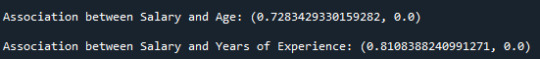
By analyzing the association between Salary and Age and Salary and Years of Experience, we observe a positive relationship, with correlation coefficients of r = 0.728 and r = 0.810, respectively.

We can also verify that the p-value = 0, meaning that the correlation is statistically significant for both relationships.

By squaring the correlation coefficient (r2)(r^2)(r2), we can determine the proportion of variability in Salary that can be explained by Age and Years of Experience.

Salary and Age

r = 0.728 → r² = 0.5299

This means that 53% of the variability in Salary can be explained by Age.

Salary and Years of Experience

r = 0.810 → r² = 0.6561

This means that 65% of the variability in Salary can be explained by Years of Experience.

[b4kingg]

Examining the Relationship Between Student Study Hours and Test Scores: A Pearson Correlation Analysis

Introduction

In this project, I explore the relationship between the number of hours students spend studying and their test scores using Pearson's correlation coefficient. This statistical measure helps determine whether there is a linear relationship between these two quantitative variables and the strength of that relationship.

Research Question

Is there a significant correlation between the number of hours a student studies and their test scores?

Methodology

I used Python with pandas, scipy.stats, matplotlib, and seaborn libraries to analyze a dataset containing information about students' study hours and their corresponding test scores.

Python Code

import pandas as pd import numpy as np import matplotlib.pyplot as plt import seaborn as sns from scipy import stats

#Create a sample dataset (in a real scenario, you would import your data)

np.random.seed(42) # For reproducibility n = 50 # Number of students

#Generate study hours (between 1 and 10)

study_hours = np.random.uniform(1, 10, n)

#Generate test scores with a positive correlation to study hours

#Adding some random noise to make it realistic

base_score = 50 hours_effect = 5 # Each hour of study adds about 5 points on average noise = np.random.normal(0, 10, n) # Random noise with mean 0 and std 10 test_scores = base_score + (hours_effect * study_hours) + noise

#Ensure test scores are between 0 and 100

test_scores = np.clip(test_scores, 0, 100)

#Create DataFrame

data = { 'Study_Hours': study_hours, 'Test_Score': test_scores } df = pd.DataFrame(data)

#Display the first few rows of the dataset

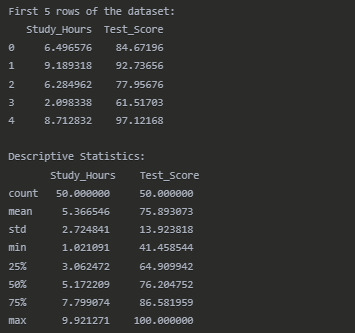
print("First 5 rows of the dataset:") print(df.head())

#Calculate descriptive statistics

print("\nDescriptive Statistics:") print(df.describe())

#Calculate Pearson correlation coefficient

r, p_value = stats.pearsonr(df['Study_Hours'], df['Test_Score']) print("\nPearson Correlation Results:") print(f"Correlation coefficient (r): {r:.4f}") print(f"P-value: {p_value:.4f}") print(f"Coefficient of determination (r²): {r**2:.4f}")

#Create a scatter plot with regression line

plt.figure(figsize=(10, 6)) sns.regplot(x='Study_Hours', y='Test_Score', data=df, line_kws={"color":"red"}) plt.title('Relationship Between Study Hours and Test Scores') plt.xlabel('Study Hours') plt.ylabel('Test Score') plt.grid(True, linestyle='--', alpha=0.7)

#Add correlation coefficient text to the plot

plt.text(1.5, 90, f'r = {r:.4f}', fontsize=12) plt.text(1.5, 85, f'r² = {r**2:.4f}', fontsize=12) plt.text(1.5, 80, f'p-value = {p_value:.4f}', fontsize=12)

plt.tight_layout() plt.show()

#Check if the correlation is statistically significant

alpha = 0.05 if p_value < alpha: significance = "statistically significant" else: significance = "not statistically significant"

print(f"\nThe correlation between study hours and test scores is {significance} at the {alpha} level.")

#Interpret the strength of the correlation

if abs(r) < 0.3: strength = "weak" elif abs(r) < 0.7: strength = "moderate" else: strength = "strong"

print(f"The correlation coefficient of {r:.4f} indicates a {strength} positive relationship.") print(f"The coefficient of determination (r²) of {r2:.4f} suggests that {(r2 * 100):.2f}% of the") print(f"variation in test scores can be explained by variation in study hours.")

Results

Dataset Overview

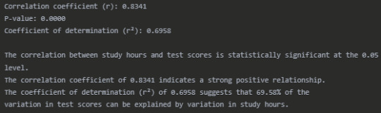
Pearson Correlation Results

Interpretation

The Pearson correlation analysis reveals a strong positive relationship (r = 0.8341) between the number of hours students spend studying and their test scores. This correlation is statistically significant (p < 0.0001), indicating that the relationship observed is unlikely to have occurred by chance.

The scatter plot visually confirms this strong positive association, with students who study more hours generally achieving higher test scores. The regression line shows the overall trend of this relationship.

The coefficient of determination (r² = 0.6958) tells us that approximately 69.58% of the variability in test scores can be explained by differences in study hours. This suggests that study time is an important factor in determining test performance, although other factors not measured in this analysis account for the remaining 30.42% of the variation.

These findings have practical implications for students and educators. They support the conventional wisdom that increased study time generally leads to better academic performance. However, the presence of unexplained variance suggests that other factors such as study quality, prior knowledge, learning environment, or individual learning styles may also play significant roles in determining test outcomes.

Conclusion

This analysis demonstrates a strong, statistically significant positive correlation between study hours and test scores. The substantial coefficient of determination suggests that encouraging students to allocate more time to studying could be an effective strategy for improving academic performance, though it's not the only factor that matters. Future research could explore additional variables that might contribute to the unexplained variance in test scores.