#pandas duplicate rows removal

[ckgupta07]

Data Analyst Interview Questions: A Comprehensive Guide

Preparing for an interview as a Data Analyst is difficult, given the broad skills needed. Technical skill, business knowledge, and problem-solving abilities are assessed by interviewers in a variety of ways. This guide will assist you in grasping the kind of questions that will be asked and how to answer them.

By mohammed hassan on Pixabay

General Data Analyst Interview Questions

These questions help interviewers assess your understanding of the role and your basic approach to data analysis.

Can you describe what a Data Analyst does? A Data Analyst collects, processes, and analyzes data to help businesses make data-driven decisions and identify trends or patterns.

What are the key responsibilities of a Data Analyst? Responsibilities include data collection, data cleaning, exploratory data analysis, reporting insights, and collaborating with stakeholders.

What tools are you most familiar with? Say tools like Excel, SQL, Python, Tableau, Power BI, and describe how you have used them in past projects.

What types of data? Describe structured, semi-structured, and unstructured data using examples such as databases, JSON files, and pictures or videos.

Technical Data Analyst Interview Questions

Technical questions evaluate your tool knowledge, techniques, and your ability to manipulate and interpret data.

What is the difference between SQL's inner join and left join? The inner join gives only the common rows between tables, whereas a left join gives all rows of the left table as well as corresponding ones of the right.

How do you deal with missing data in a dataset? Methods are either removing rows, mean/median imputation, or forward-fill/backward-fill depending on context and proportion of missing data.

Can you describe normalization and why it's significant? Normalization minimizes data redundancy and enhances data integrity by structuring data effectively between relational tables.

What are some Python libraries that are frequently used for data analysis? Libraries consist of Pandas for data manipulation, NumPy for numerical computations, Matplotlib/Seaborn for data plotting, and SciPy for scientific computing.

How would you construct a query to discover duplicate values within a table? Use a GROUP BY clause with a HAVING COUNT(*) > 1 to find duplicate records according to one or more columns.

Behavioral and Situational Data Analyst Interview Questions

These assess your soft skills, work values, and how you deal with actual situations.

Describe an instance where you managed a challenging stakeholder. Describe how you actively listened, recognized their requirements, and provided insights that supported business objectives despite issues with communication.

Tell us about a project in which you needed to analyze large datasets. Describe how you broke the dataset down into manageable pieces, what tools you used, and what you learned from the analysis.

Read More....

[globosetechnologysolutionspvt]

How to Clean and Preprocess AI Data Sets for Better Results

Introduction

Artificial Intelligence Dataset (AI) models depend on high-quality data to produce accurate and dependable outcomes. Nevertheless, raw data frequently contains inconsistencies, errors, and extraneous information, which can adversely affect model performance. Effective data cleaning and preprocessing are critical steps to improve the quality of AI datasets, thereby ensuring optimal training and informed decision-making.

The Importance of Data Cleaning and Preprocessing

The quality of data has a direct impact on the effectiveness of AI and machine learning models. Inadequately processed data can result in inaccurate predictions, biased results, and ineffective model training. By adopting systematic data cleaning and preprocessing techniques, organizations can enhance model accuracy, minimize errors, and improve overall AI performance.

Procedures for Cleaning and Preprocessing AI Datasets

1. Data Collection and Analysis

Prior to cleaning, it is essential to comprehend the source and structure of your data. Identify key attributes, missing values, and any potential biases present in the dataset.

2. Addressing Missing Data

Missing values can hinder model learning. Common approaches to manage them include:

Deletion: Removing rows or columns with a significant number of missing values.

Imputation: Filling in missing values using methods such as mean, median, mode, or predictive modeling.

Interpolation: Estimating missing values based on existing trends within the dataset.

3. Eliminating Duplicates and Irrelevant Data

Duplicate entries can distort AI training outcomes. It is important to identify and remove duplicate records to preserve data integrity. Furthermore, eliminate irrelevant or redundant features that do not enhance the model’s performance.

4. Managing Outliers and Noisy Data

Outliers can negatively impact model predictions. Employ methods such as

The Z-score or Interquartile Range (IQR) approach to identify and eliminate extreme values.

Smoothing techniques, such as moving averages, to mitigate noise.

5. Data Standardization and Normalization

To maintain uniformity across features, implement:

Standardization: Adjusting data to achieve a mean of zero and a variance of one.

Normalization: Scaling values to a specified range (e.g., 0 to 1) to enhance model convergence.

6. Encoding Categorical Variables

Machine learning models perform optimally with numerical data. Transform categorical variables through:

One-hot encoding for nominal categories.

Label encoding for ordinal categories.

7. Feature Selection and Engineering

Minimizing the number of features can enhance model performance. Utilize techniques such as:

Principal Component Analysis (PCA) for reducing dimensionality.

Feature engineering to develop significant new features from existing data.

8. Data Partitioning for Training and Testing

Effective data partitioning is essential for an unbiased assessment of model performance. Typical partitioning strategies include:

An 80-20 split, allocating 80% of the data for training purposes and 20% for testing.

Utilizing cross-validation techniques to enhance the model's ability to generalize.

Tools for Data Cleaning and Preprocessing

A variety of tools are available to facilitate data cleaning, such as:

Pandas and NumPy, which are useful for managing missing data and performing transformations.

Scikit-learn, which offers preprocessing methods like normalization and encoding.

OpenCV, specifically for improving image datasets.

Tensor Flow and Pytorch, which assist in preparing datasets for deep learning applications.

Conclusion

The processes of cleaning and preprocessing AI datasets are vital for achieving model accuracy and operational efficiency. By adhering to best practices such as addressing missing values, eliminating duplicates, normalizing data, and selecting pertinent features, organizations can significantly improve AI performance and minimize biases. Utilizing sophisticated data cleaning tools can further streamline these efforts, resulting in more effective and dependable AI models. 

For professional AI dataset solutions, visit Globose Technology Solutions to enhance your machine learning initiatives.

[gloriousfestgentlemen02]

```markdown

SEO Data Cleaning Scripts: Boost Your Website's Performance with Clean Data

In the world of Search Engine Optimization (SEO), data is king. However, dirty or inaccurate data can significantly hinder your website's performance and ranking. This article will guide you through the importance of data cleaning in SEO and introduce you to some effective scripts that can help streamline this process.

Why Data Cleaning Matters in SEO

Data cleaning is crucial for several reasons:

1. Improves Accuracy: By removing duplicates, correcting errors, and standardizing formats, you ensure that your analytics tools provide accurate insights.

2. Enhances Efficiency: Clean data allows your SEO strategies to be more efficient and targeted, leading to better results.

3. Boosts Credibility: Presenting clean, well-organized data to clients or stakeholders boosts credibility and trust.

Common Issues in SEO Data

Before diving into the scripts, let's identify some common issues that often need addressing:

Duplicate Entries: These can skew metrics and make it difficult to get a clear picture of your website's performance.

Incorrect Formatting: Different date formats, inconsistent capitalization, and other formatting issues can lead to misinterpretation of data.

Missing Values: Null or missing data points can cause significant problems when analyzing trends or making decisions.

Scripts for Data Cleaning

Here are a few Python scripts that can help you clean your SEO data effectively:

1. Remove Duplicates

```python

import pandas as pd

Load your data

data = pd.read_csv('your_data.csv')

Remove duplicates

cleaned_data = data.drop_duplicates()

Save cleaned data

cleaned_data.to_csv('cleaned_data.csv', index=False)

```

2. Standardize Date Formats

```python

import pandas as pd

Load your data

data = pd.read_csv('your_data.csv')

Convert 'date' column to datetime format

data['date'] = pd.to_datetime(data['date'], errors='coerce')

Format dates consistently

data['date'] = data['date'].dt.strftime('%Y-%m-%d')

Save cleaned data

data.to_csv('cleaned_data.csv', index=False)

```

3. Handle Missing Values

```python

import pandas as pd

data = pd.read_csv('your_data.csv')

Fill missing values with a specific value or method

data.fillna(value=0, inplace=True)

Alternatively, drop rows with missing values

data.dropna(inplace=True)

data.to_csv('cleaned_data.csv', index=False)

```

Conclusion

Data cleaning is an essential part of any successful SEO strategy. By using these scripts, you can ensure that your data is accurate, consistent, and ready for analysis. What are some other challenges you face with SEO data? Share your thoughts and experiences in the comments below!

```

```

加飞机@yuantou2048

ETPU Machine

蜘蛛池出租

[learning-code-ficusoft]

Preparing Data for Training in Machine Learning

Preparing data is a crucial step in building a machine learning model. Poorly processed data can lead to inaccurate predictions and inefficient models. 

Below are the key steps involved in preparing data for training. 

Understanding and Collecting Data Before processing, ensure that the data is relevant, diverse, and representative of the problem you’re solving. 

✅ Sources — Data can come from databases, APIs, files (CSV, JSON), or real-time streams. 

✅ Data Types — Structured (tables, spreadsheets) or unstructured (text, images, videos). 

✅ Labeling — For supervised learning, ensure data is properly labeled. 

2. Data Cleaning and Preprocessing

 Raw data often contains errors, missing values, and inconsistencies that must be addressed. Key Steps: 

✔ Handling Missing Values — Fill with mean/median (numerical) or mode (categorical), or drop incomplete rows. 

✔ Removing Duplicates — Avoid bias by eliminating redundant records. 

✔ Handling Outliers — Use statistical methods (Z-score, IQR) to detect and remove extreme values. 

✔ Data Type Conversion — Ensure consistency in numerical, categorical, and date formats. 

3. Feature Engineering Transforming raw data into meaningful features improves model performance. 

Techniques: 

📌 Normalization & Standardization — Scale numerical features to bring them to the same range. 

📌 One-Hot Encoding — Convert categorical variables into numerical form. 

📌 Feature Selection — Remove irrelevant or redundant features using correlation analysis or feature importance. 

📌 Feature Extraction — Create new features (e.g., extracting time-based trends from timestamps). 4. Splitting Data into Training, Validation, and Testing Sets To evaluate model performance effectively, divide data into: Training Set (70–80%) — Used for training the model. 

Validation Set (10–15%) — Helps tune hyperparameters and prevent overfitting. Test Set (10–15%) — Evaluates model performance on unseen data. 

📌 Stratified Sampling — Ensures balanced distribution of classes in classification tasks.

 5. Data Augmentation (For Image/Text Data) 

If dealing with images or text, artificial expansion of the dataset can improve model generalization. 

✔ Image Augmentation — Rotate, flip, zoom, adjust brightness. 

✔ Text Augmentation — Synonym replacement, back-translation, text shuffling. 

6. Data Pipeline Automation For large datasets, 

use ETL (Extract, Transform, Load) pipelines or tools like Apache Airflow, AWS Glue, or Pandas to automate data preparation.

WEBSITE: https://www.ficusoft.in/deep-learning-training-in-chennai/

[fromdevcom]

Pandas DataFrame Cleanup: Master the Art of Dropping Columns Data cleaning and preprocessing are crucial steps in any data analysis project. When working with pandas DataFrames in Python, you'll often encounter situations where you need to remove unnecessary columns to streamline your dataset. In this comprehensive guide, we'll explore various methods to drop columns in pandas, complete with practical examples and best practices. Understanding the Basics of Column Dropping Before diving into the methods, let's understand why we might need to drop columns: Remove irrelevant features that don't contribute to analysis Eliminate duplicate or redundant information Clean up data before model training Reduce memory usage for large datasets Method 1: Using drop() - The Most Common Approach The drop() method is the most straightforward way to remove columns from a DataFrame. Here's how to use it: pythonCopyimport pandas as pd # Create a sample DataFrame df = pd.DataFrame( 'name': ['John', 'Alice', 'Bob'], 'age': [25, 30, 35], 'city': ['New York', 'London', 'Paris'], 'temp_col': [1, 2, 3] ) # Drop a single column df = df.drop('temp_col', axis=1) # Drop multiple columns df = df.drop(['city', 'age'], axis=1) The axis=1 parameter indicates we're dropping columns (not rows). Remember that drop() returns a new DataFrame by default, so we need to reassign it or use inplace=True. Method 2: Using del Statement - The Quick Solution For quick, permanent column removal, you can use Python's del statement: pythonCopy# Delete a column using del del df['temp_col'] Note that this method modifies the DataFrame directly and cannot be undone. Use it with caution! Method 3: Drop Columns Using pop() - Remove and Return The pop() method removes a column and returns it, which can be useful when you want to store the removed column: pythonCopy# Remove and store a column removed_column = df.pop('temp_col') Advanced Column Dropping Techniques Dropping Multiple Columns with Pattern Matching Sometimes you need to drop columns based on patterns in their names: pythonCopy# Drop columns that start with 'temp_' df = df.drop(columns=df.filter(regex='^temp_').columns) # Drop columns that contain certain text df = df.drop(columns=df.filter(like='unused').columns) Conditional Column Dropping You might want to drop columns based on certain conditions: pythonCopy# Drop columns with more than 50% missing values threshold = len(df) * 0.5 df = df.dropna(axis=1, thresh=threshold) # Drop columns of specific data types df = df.select_dtypes(exclude=['object']) Best Practices for Dropping Columns Make a Copy First pythonCopydf_clean = df.copy() df_clean = df_clean.drop('column_name', axis=1) Use Column Lists for Multiple Drops pythonCopycolumns_to_drop = ['col1', 'col2', 'col3'] df = df.drop(columns=columns_to_drop) Error Handling pythonCopytry: df = df.drop('non_existent_column', axis=1) except KeyError: print("Column not found in DataFrame") Performance Considerations When working with large datasets, consider these performance tips: Use inplace=True to avoid creating copies: pythonCopydf.drop('column_name', axis=1, inplace=True) Drop multiple columns at once rather than one by one: pythonCopy# More efficient df.drop(['col1', 'col2', 'col3'], axis=1, inplace=True) # Less efficient df.drop('col1', axis=1, inplace=True) df.drop('col2', axis=1, inplace=True) df.drop('col3', axis=1, inplace=True) Common Pitfalls and Solutions Dropping Non-existent Columns pythonCopy# Use errors='ignore' to skip non-existent columns df = df.drop('missing_column', axis=1, errors='ignore') Chain Operations Safely pythonCopy# Use method chaining carefully df = (df.drop('col1', axis=1) .drop('col2', axis=1) .reset_index(drop=True)) Real-World Applications Let's look at a practical example of cleaning a dataset: pythonCopy# Load a messy dataset df = pd.read_csv('raw_data.csv')

# Clean up the DataFrame df_clean = (df.drop(columns=['unnamed_column', 'duplicate_info']) # Remove unnecessary columns .drop(columns=df.filter(regex='^temp_').columns) # Remove temporary columns .drop(columns=df.columns[df.isna().sum() > len(df)*0.5]) # Remove columns with >50% missing values ) Integration with Data Science Workflows When preparing data for machine learning: pythonCopy# Drop target variable from features X = df.drop('target_variable', axis=1) y = df['target_variable'] # Drop non-numeric columns for certain algorithms X = X.select_dtypes(include=['float64', 'int64']) Conclusion Mastering column dropping in pandas is essential for effective data preprocessing. Whether you're using the simple drop() method or implementing more complex pattern-based dropping, understanding these techniques will make your data cleaning process more efficient and reliable. Remember to always consider your specific use case when choosing a method, and don't forget to make backups of important data before making permanent changes to your DataFrame. Now you're equipped with all the knowledge needed to effectively manage columns in your pandas DataFrames. Happy data cleaning!

[sak-shi]

Ensuring Data Accuracy with Cleaning

Ensuring data accuracy with cleaning is an essential step in data preparation. Here’s a structured approach to mastering this process:

1. Understand the Importance of Data Cleaning

Data cleaning is crucial because inaccurate or inconsistent data leads to faulty analysis and incorrect conclusions. Clean data ensures reliability and robustness in decision-making processes.

2. Common Data Issues

Identify the common issues you might face:

Missing Data: Null or empty values.

Duplicate Records: Repeated entries that skew results.

Inconsistent Formatting: Variations in date formats, currency, or units.

Outliers and Errors: Extreme or invalid values.

Data Type Mismatches: Text where numbers should be or vice versa.

Spelling or Casing Errors: Variations like “John Doe” vs. “john doe.”

Irrelevant Data: Data not needed for the analysis.

3. Tools and Libraries for Data Cleaning

Python: Libraries like pandas, numpy, and pyjanitor.

Excel: Built-in cleaning functions and tools.

SQL: Using TRIM, COALESCE, and other string functions.

Specialized Tools: OpenRefine, Talend, or Power Query.

4. Step-by-Step Process

a. Assess Data Quality

Perform exploratory data analysis (EDA) using summary statistics and visualizations.

Identify missing values, inconsistencies, and outliers.

b. Handle Missing Data

Imputation: Replace with mean, median, mode, or predictive models.

Removal: Drop rows or columns if data is excessive or non-critical.

c. Remove Duplicates

Use functions like drop_duplicates() in pandas to clean redundant entries.

d. Standardize Formatting

Convert all text to lowercase/uppercase for consistency.

Standardize date formats, units, or numerical scales.

e. Validate Data

Check against business rules or constraints (e.g., dates in a reasonable range).

f. Handle Outliers

Remove or adjust values outside an acceptable range.

g. Data Type Corrections

Convert columns to appropriate types (e.g., float, datetime).

5. Automate and Validate

Automation: Use scripts or pipelines to clean data consistently.

Validation: After cleaning, cross-check data against known standards or benchmarks.

6. Continuous Improvement

Keep a record of cleaning steps to ensure reproducibility.

Regularly review processes to adapt to new challenges.

Would you like a Python script or examples using a specific dataset to see these principles in action?

[analyticsshiksha30]

What is data cleaning with pandas

Data cleaning with Pandas involves using the library's powerful functions to prepare and transform raw data into a format suitable for analysis. Raw datasets often contain inconsistencies, missing values, duplicates, or incorrect data types, which can skew results if not properly handled.

Key steps in data cleaning with Pandas include:

Handling Missing Data: Missing values can be addressed using methods such as fillna() to replace them with a default value or the mean/median of a column, or by using dropna() to remove rows or columns with missing values.

Removing Duplicates: Duplicated rows can be identified and removed using drop_duplicates(), which ensures each record is unique and prevents skewed analysis.

Data Type Conversion: Incorrect data types can cause issues during analysis. The astype() function allows you to convert columns to appropriate types, such as changing strings to dates or numbers.

Filtering and Renaming Columns: You can filter or rename columns using filter() or rename(), making the dataset easier to manage and understand.

Standardizing Data: Inconsistent formatting, such as varying text capitalization, can be standardized using methods like str.lower() or str.strip(). Handling Outliers: Pandas can also help in identifying and handling outliers by applying functions like describe() to detect unusual values.

[asquaretechnologies]

Beginner’s Guide: Data Analysis with Pandas

Data analysis is the process of sorting through all the data, looking for patterns, connections, and interesting things. It helps us make sense of information and use it to make decisions or find solutions to problems. When it comes to data analysis and manipulation in Python, the Pandas library reigns supreme. Pandas provide powerful tools for working with structured data, making it an indispensable asset for both beginners and experienced data scientists.

What is Pandas?

Pandas is an open-source Python library for data manipulation and analysis. It is built on top of NumPy, another popular numerical computing library, and offers additional features specifically tailored for data manipulation and analysis. There are two primary data structures in Pandas:

• Series: A one-dimensional array capable of holding any type of data.

• DataFrame: A two-dimensional labeled data structure similar to a table in relational databases.

It allows us to efficiently process and analyze data, whether it comes from any file types like CSV files, Excel spreadsheets, SQL databases, etc.

How to install Pandas?

We can install Pandas using the pip command. We can run the following codes in the terminal.

After installing, we can import it using:

How to load an external dataset using Pandas?

Pandas provide various functions for loading data into a data frame. One of the most commonly used functions is pd.read_csv() for reading CSV files. For example:

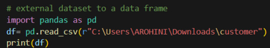
The output of the above code is:

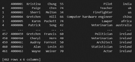
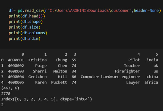
Once your data is loaded into a data frame, you can start exploring it. Pandas offers numerous methods and attributes for getting insights into your data. Here are a few examples:

df.head(): View the first few rows of the DataFrame.

df.tail(): View the last few rows of the DataFrame.

http://df.info(): Get a concise summary of the DataFrame, including data types and missing values.

df.describe(): Generate descriptive statistics for numerical columns.

df.shape: Get the dimensions of the DataFrame (rows, columns).

df.columns: Access the column labels of the DataFrame.

df.dtypes: Get the data types of each column.

In data analysis, it is essential to do data cleaning. Pandas provide powerful tools for handling missing data, removing duplicates, and transforming data. Some common data-cleaning tasks include:

Handling missing values using methods like df.dropna() or df.fillna().

Removing duplicate rows with df.drop_duplicates().

Data type conversion using df.astype().

Renaming columns with df.rename().

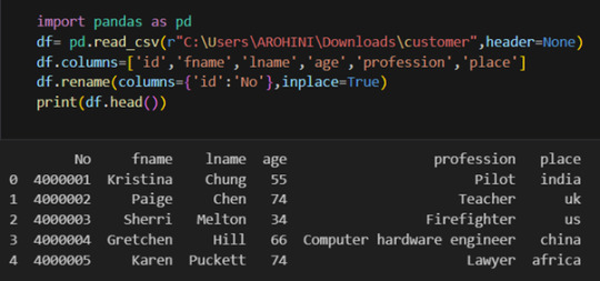
Pandas excels in data manipulation tasks such as selecting subsets of data, filtering rows, and creating new columns. Here are a few examples:

Selecting columns: df[‘column_name’] or df[[‘column1’, ‘column2’]].

Filtering rows based on conditions: df[df[‘column’] > value].

Sorting data: df.sort_values(by=’column’).

Grouping data: df.groupby(‘column’).mean().

With data cleaned and prepared, you can use Pandas to perform various analyses. Whether you’re computing statistics, performing exploratory data analysis, or building predictive models, Pandas provides the tools you need. Additionally, Pandas integrates seamlessly with other libraries such as Matplotlib and Seaborn for data visualization

[data-science-lovers]

Dealing with Duplicate Rows in Big-Data

[learning-code-ficusoft]

Data Analysis with Python: A Beginner’s Guide to Pandas

Data Analysis with Python: 

A Beginner’s Guide to Pandas Pandas is a foundational library in Python for data analysis, offering robust tools to work with structured data. 

It simplifies tasks like data cleaning, exploration, and transformation, making it indispensable for beginners and experts alike. 

What is Pandas?

 Pandas is an open-source Python library built for:

 Data Manipulation: Transforming and restructuring datasets. 

Data Analysis: Aggregating, summarizing, and deriving insights from data. Handling Tabular Data: Easily working with structured data, such as tables or CSV files. 

By leveraging Pandas, analysts can focus on solving problems rather than worrying about low-level data-handling complexities. 

Core Concepts in Pandas Data Structures:

 Series: A one-dimensional array with labeled indices. 

Example Use Case: 

Storing a list of items with labels (e.g., prices of products). 

DataFrame: A two-dimensional structure with labeled rows and columns. 

Example Use Case: Representing a table with rows as observations and columns as attributes. 

Data Handling: Loading Data: Pandas supports importing data from various sources like CSV, Excel, SQL databases, and more. 

Data Cleaning: 

Removing duplicates, handling missing values, and correcting data types. 

Data Transformation: 

Filtering, sorting, and applying mathematical or logical operations to reshape datasets. 

Exploratory Data Analysis (EDA): With Pandas, analyzing data trends and patterns becomes simple. 

Examples include: Summarizing data with describe(). Grouping and aggregating data using groupby().

 Why Use Pandas for Data Analysis?

 Ease of Use: 

Pandas provides intuitive, high-level methods for working with data, reducing the need for complex programming. 

Versatility: It supports handling various data formats and seamlessly integrates with other libraries like NumPy, Matplotlib, and Seaborn. Efficiency: Built on top of NumPy, Pandas ensures fast data operations and processing. 

Key Advantages for Beginners Readable Code: 

Pandas uses simple, readable syntax, making it easy for beginners to adopt. Comprehensive 

Documentation: Extensive resources and community support help users quickly learn the library. 

Real-World Applications: Pandas is widely used in industries for financial analysis, machine learning, and business intelligence. 

Theoretical Importance of Pandas Pandas abstracts complex data manipulation into easy-to-use methods, empowering users to: Handle data from raw formats to structured forms. Perform detailed analysis without extensive programming effort. 

Build scalable pipelines for data processing and integration. 

This makes Pandas an essential tool for anyone stepping into the world of data analysis with Python.

WEBSITE: https://www.ficusoft.in/python-training-in-chennai/

[lukaspyblog]

Generating a Correlation Coefficient

In This analysis i want to check if the opponents rating in a Chess.com Grandmaster match is influenced by the players rating. I got my dataset from Kaggle:

I then import the most important libraries and read my dataset.

```python

import pandas

import seaborn

import scipy

import matplotlib.pyplot as plt

data = pandas.read_csv('chess.csv', low_memory=False)

```

```python

print(data)

```

           time_control             end_time  rated time_class  rules  \

    0             300+1  2021-06-19 11:40:40   True      blitz  chess  

    1             300+1  2021-06-19 11:50:06   True      blitz  chess  

    2             300+1  2021-06-19 12:01:17   True      blitz  chess  

    3             300+1  2021-06-19 12:13:05   True      blitz  chess  

    4             300+1  2021-06-19 12:28:54   True      blitz  chess  

    ...             ...                  ...    ...        ...    ...  

    859365           60  2021-12-31 16:58:31   True     bullet  chess  

    859366           60  2021-04-20 01:12:33   True     bullet  chess  

    859367           60  2021-04-20 01:14:49   True     bullet  chess  

    859368           60  2021-04-20 01:17:00   True     bullet  chess  

    859369           60  2021-04-20 01:19:13   True     bullet  chess  

                gm_username   white_username  white_rating white_result  \

    0                 123lt     vaishali2001          2658          win  

    1                 123lt            123lt          2627          win  

    2                 123lt     vaishali2001          2641      timeout  

    3                 123lt            123lt          2629      timeout  

    4                 123lt     vaishali2001          2657          win  

    ...                 ...              ...           ...          ...  

    859365        zuraazmai      redblizzard          2673          win  

    859366  zvonokchess1996       TampaChess         ��2731     resigned  

    859367  zvonokchess1996  zvonokchess1996          2892          win  

    859368  zvonokchess1996       TampaChess          2721      timeout  

    859369  zvonokchess1996  zvonokchess1996          2906          win  

             black_username  black_rating black_result  

    0                 123lt          2601     resigned  

    1          vaishali2001          2649     resigned  

    2                 123lt          2649          win  

    3          vaishali2001          2649          win  

    4                 123lt          2611     resigned  

    ...                 ...           ...          ...  

    859365        ZURAAZMAI          2664      timeout  

    859366  zvonokchess1996          2884          win  

    859367       TampaChess          2726   checkmated  

    859368  zvonokchess1996          2899          win  

    859369       TampaChess          2717     resigned  

    [859370 rows x 12 columns]

```python

dup = data[data.duplicated()].shape[0]

print(f"There are {dup} duplicate entries among {data.shape[0]} entries in this dataset.")

#not needed as no duplicates

#data_clean = data.drop_duplicates(keep='first',inplace=True)

#print(f"\nAfter removing duplicate entries there are {data_clean.shape[0]} entries in this dataset.")

```

    There are 0 duplicate entries among 859366 entries in this dataset.

Even though the dataset is huge there are no duplicates so i can now check make my plot.

As there are many entires i have to lower the transparency of all points so the Outliers do not affect the overall picture

```python

scat1 = seaborn.regplot(x="white_rating",

                        y="black_rating",

                        fit_reg=True, data=data,

                        scatter_kws={'alpha':0.002})

plt.xlabel('White Rating')

plt.ylabel('Black Rating')

plt.title('Scatterplot for the Association Between the Elo Rate of 2 players')

```

    Text(0.5, 1.0, 'Scatterplot for the Association Between the Elo Rate of 2 players')


```python

print ('association between White Rating and Black Rating')

print (scipy.stats.pearsonr(data['white_rating'], data['black_rating']))

```

    association between White Rating and Black Rating

    PearsonRResult(statistic=0.46087882769619515, pvalue=0.0)

The statistics is fairly high and the P-Value is so low that it actually shows a 0 so we can confidently reject the null hypothesis. We can therefore conclude that there is a statistical relevance between the Player Rating and it's opponent.

The r^2 value is 0.21 therefore we can conclude that 21% of the variablility in the opponents rating can be explained by the Players rating.

[sak-shi]

The Foundation of Clean Data Analysis

Clean data is the cornerstone of accurate and reliable data analysis. A robust foundation in data cleaning ensures that your insights are valid, consistent, and actionable. Here’s an outline of the foundational steps for clean data analysis:

1. Understanding the Dataset

Familiarize Yourself with the Data Understand the context of the dataset, including its purpose, variables, and expected outcomes. Tools: Data dictionaries, documentation, or domain expertise.

Inspect the Data Use methods like .head(), .info(), and .describe() in Python to gain an overview of the dataset's structure and summary statistics.

2. Identifying and Handling Missing Data

Locate Missing Data Identify missing values using functions like .isnull().sum() in Python. Visualization: Heatmaps (e.g., Seaborn) can highlight missing data patterns.

Strategies to Handle Missing Data

Removal: Drop rows or columns with excessive missing values.

Imputation: Fill missing values using statistical methods (mean, median, mode) or predictive models.

3. Addressing Outliers

Detect Outliers Use visualizations like boxplots or statistical methods like Z-scores and IQR to identify outliers.

Handle Outliers Options include capping, transformation, or removal, depending on the context of the analysis.

4. Resolving Inconsistencies

Standardize Data Formats Ensure consistency in formats (e.g., date formats, text capitalization, units of measurement). Example: Converting all text to lowercase using .str.lower() in Python.

Validate Entries Check for and correct invalid entries like negative ages or typos in categorical data.

5. Dealing with Duplicates

Detect Duplicates Use methods like .duplicated() to identify duplicate rows.

Handle Duplicates Drop duplicates unless they are meaningful for the analysis.

6. Ensuring Correct Data Types

Verify Data Types Check that variables have appropriate types (e.g., integers for counts, strings for categories).

Convert Data Types Use type-casting functions like astype() in Python to fix mismatched data types.

7. Data Transformation

Feature Scaling Apply normalization or standardization for numerical features used in machine learning. Techniques: Min-Max scaling or Z-score normalization.

Encoding Categorical Variables Use one-hot encoding or label encoding for categorical features.

Key Tools for Data Cleaning:

Libraries: Pandas, NumPy, Seaborn, Matplotlib (for Python users).

Software: Excel, OpenRefine, or specialized ETL tools like Talend or Alteryx.

By mastering these foundational steps, you’ll ensure your data is clean, consistent, and ready for exploration and analysis. Would you like more detailed guidance or code examples for any of these steps?

[ghorbelma]

Data Management and Visualization Making Data Management Decisions

DataSet: Gapminder

Variable: countries, democracy score, employ rate and female employ rate.

some democracy score are missings, I displayed the frequency by quantile.

employ rate values are correct (between 0 and 100%) but some rows all empty

female employ rate has some dummy values (when i displayed the quantiles, the last quantiles end value is greater than 100%), some data is missing

I checked column by column if there is any empty cells (I am able to conduct analysis between the variables only if for a given countries all the figures are non empty)

I checked if there is any dummy variable employ rate and female rate should  be between 0 and 100% and replaced it by Nan

Finally I construct  a new dataframe with only a rows containing a non empty and valide Data

######THE CODE####################

import pandas import numpy

data =pandas.read_csv("Gapminder.csv",";")

print ("Total Contries: " + str(len(data))) print ("Total Columns "+ str(len(data.columns)))

#convert_objects seems deprecated, use to_numeric instead #data["employrate"]= data["employrate"].convert_objects(convert_numeric=True) #NAN are kept #First just browse all columns date, then look for some subgroup (sample) #data sorted by value (indexof)and not by the frequency of occurence

##############POLITYSCORE##############

data["polityscore"]= pandas.to_numeric(data["polityscore"], errors='coerce' )

democracy_Score_Data = data["polityscore"].copy()

democracy_Score_Frequency =(pandas.qcut( democracy_Score_Data,4,duplicates='drop', labels=["0-25%","25%-50%","50%-75%","75%-100%"])).value_counts(sort=True,dropna =True).sort_index() print('\n') print('Democracy score summary data') print(democracy_Score_Data.describe()) print('\n') print ("Democracy score quantile") print (democracy_Score_Frequency)

##############EMPLOY RATE############## print('\n') print ("Count for employrate: 2007 total employees age 15+ (% of population)") data["employrate"]= pandas.to_numeric(data["employrate"], errors='coerce' ) data_employRate_discrete=pandas.cut(data["employrate"],10)

employ_Rate_Frequency =data_employRate_discrete.value_counts(sort=True,dropna =False).sort_index()

print (employ_Rate_Frequency)

##############FEMALEEMPLOYRATE############## print ("Count for female employrate: 2007 total female employees age 15+ (% of population)") data["femaleemployrate"]= pandas.to_numeric(data["femaleemployrate"], errors='coerce' )

femaleEmployRateData = data["femaleemployrate"].copy()

data_femaleemployRate_beforeCorrection=pandas.qcut(data["femaleemployrate"],10) female_employ_Rate_Frequency_beforeCorrection =data_femaleemployRate_beforeCorrection.value_counts(sort=True,dropna =False).sort_index() print('\n') print ("Female employ rate, should be between 0 and 100") print (female_employ_Rate_Frequency_beforeCorrection)

#femaleEmployRateData=femaleEmployRateData.apply (lambda  x:[x if x <= 100 else numpy.NaN]) femaleEmployRateData.values[femaleEmployRateData > 100] = numpy.NaN data_femaleemployRate_afterCorrection=pandas.qcut(femaleEmployRateData,10)

female_employ_Rate_Frequency_afterCorrection =data_femaleemployRate_afterCorrection.value_counts(sort=True,dropna =False).sort_index() print('\n') print ("Female employ rate, all dummy values greater than 100 were removed") print (female_employ_Rate_Frequency_afterCorrection)

#########  BUILDING The DATA FRAME TO USE######################## print('\n') print("Constructing the data frame to be used from the gapminder data") # subset variables in new data frame, sub1 sub1=data[['country','polityscore', 'employrate', 'femaleemployrate' ]] print('\n') print ('Check the last 10 element of the dataset, some dummies or missing are there') print(sub1.tail(10))

def CorrectEmployRate (row):   if row['femaleemployrate'] > 100   :      return numpy.NaN   else:      return  row['femaleemployrate']

sub1['femaleemployrate']=sub1.apply (lambda row: CorrectEmployRate (row),axis=1) print('\n') print('Dummy female rate after correction again displaying last 10 elements') print(sub1.tail(10))

print('\n') print('The Data Frame with all the correct Data') print('Keep only data with finite value') sub2 = sub1[numpy.isfinite(sub1['femaleemployrate']) & numpy.isfinite(sub1['polityscore']) &numpy.isfinite(sub1['employrate'])] print(sub2.tail(10))

print('\n') print('--------REMAINING DATA SUMMARY------------------') print(sub2.describe())

############The OUTPUT###########

Total Contries: 213 Total Columns 17

Democracy score summary data count   157.000000 mean      3.766691 std       6.244515 min     -10.000000 25%      -1.000000 50%       6.000000 75%       9.000000 max      10.000000 Name: polityscore, dtype: float64

Democracy score quantile 0-25%       43 25%-50%     36 50%-75%     45 75%-100%    33 Name: polityscore, dtype: int64

Count for employrate: 2007 total employees age 15+ (% of population) (4.657, 12.582]      5 (12.582, 20.429]     1 (20.429, 28.275]     1 (28.275, 36.121]     1 (36.121, 43.968]    12 (43.968, 51.814]    32 (51.814, 59.661]    50 (59.661, 67.507]    44 (67.507, 75.354]    18 (75.354, 83.2]      13 NaN                 36 Name: employrate, dtype: int64 Count for female employrate: 2007 total female employees age 15+ (% of population)

Female employ rate, should be between 0 and 100 (11.299000000000001, 30.34]    18 (30.34, 37.5]                  18 (37.5, 41.16]                  18 (41.16, 45.2]                  17 (45.2, 48.45]                  18 (48.45, 51.3]                  20 (51.3, 54.69]                  15 (54.69, 60.82]                 18 (60.82, 73.12]                 18 (73.12, 9666891666.667]        18 NaN                            35 Name: femaleemployrate, dtype: int64

Female employ rate, all dummy values greater than 100 were removed (11.299000000000001, 30.19]    17 (30.19, 37.2]                  17 (37.2, 40.24]                  17 (40.24, 43.92]                 17 (43.92, 47.1]                  18 (47.1, 50.64]                  16 (50.64, 53.66]                 17 (53.66, 58.22]                 17 (58.22, 66.7]                  17 (66.7, 83.3]                   17 NaN                            43 Name: femaleemployrate, dtype: int64

Constructing the data frame to be used from the gapminder data

Check the last 10 element of the dataset, some dummies or missing are there                country  polityscore  employrate  femaleemployrate 203       United States    10.000000   62.299999         56.000000 204             Uruguay    10.000000   57.500000         46.000000 205          Uzbekistan    -9.000000   57.500000         52.599998 206             Vanuatu          nan         nan               nan 207           Venezuela    -3.000000   59.900002         45.799999 208             Vietnam    -7.000000   71.000000         67.599998 209  West Bank and Gaza          nan   32.000000         11.300000 210               Yemen          nan    6.265789  234864666.666667 211              Zambia     7.000000   61.000000         53.500000 212            Zimbabwe     1.000000   66.800003         58.099998

Dummy female rate after correction again displaying last 10 elements                country  polityscore  employrate  femaleemployrate 203       United States    10.000000   62.299999         56.000000 204             Uruguay    10.000000   57.500000         46.000000 205          Uzbekistan    -9.000000   57.500000         52.599998 206             Vanuatu          nan         nan               nan 207           Venezuela    -3.000000   59.900002         45.799999 208             Vietnam    -7.000000   71.000000         67.599998 209  West Bank and Gaza          nan   32.000000         11.300000 210               Yemen          nan    6.265789               nan 211              Zambia     7.000000   61.000000         53.500000 212            Zimbabwe     1.000000   66.800003         58.099998

The Data Frame with all the correct Data Keep only data with finite value                  country  polityscore  employrate  femaleemployrate 200               Ukraine     7.000000   54.400002         49.400002 201  United Arab Emirates    -8.000000   75.199997         37.299999 202        United Kingdom    10.000000   59.299999         53.099998 203         United States    10.000000   62.299999         56.000000 204               Uruguay    10.000000   57.500000         46.000000 205            Uzbekistan    -9.000000   57.500000         52.599998 207             Venezuela    -3.000000   59.900002         45.799999 208               Vietnam    -7.000000   71.000000         67.599998 211                Zambia     7.000000   61.000000         53.500000 212              Zimbabwe     1.000000   66.800003         58.099998

--------REMAINING DATA SUMMARY------------------       polityscore  employrate  femaleemployrate count   152.000000  152.000000        152.000000 mean      3.736842   59.563816         48.292763 std       6.319042   10.127999         14.745075 min     -10.000000   37.400002         12.400000 25%      -2.000000   52.650001         39.599998 50%       6.500000   58.900002         48.549999 75%       9.000000   65.025000         56.325001 max      10.000000   83.199997         83.300003

[sweetpizzacheesecake]

Week 3 Peer Graded Assignment

1. Program (Python Code)

#Import relevant libraries import pandas as pd import numpy as np

#Read data from CSV file data = pd.read_csv('nesarc_pds_ae1.csv', low_memory=(False))

#Uppercase all dataframe column names data.columns = map(str.upper, data.columns)

#Display counts and percentage tables for 3 variables #Major depression tables: print('Frequency Table 1: Major Depression in Subjects') print('Data Management: Data already in desired format. No additional steps required') print("Count of subjects experiencing major depression in the last 12 months (no = 0, yes = 1)") c1 = data['MAJORDEP12'].value_counts(sort=False) print(c1,'\n')

print('Percent of subjects experiencing major depression in the last 12 months (no = 0, yes = 1)') p1 = data['MAJORDEP12'].value_counts(sort=False, normalize=True) print(p1,'\n \n')

#Data management- change index to actual dollars (in thousands) sub0=data.copy() recode0={1:0, 2:5, 3:8, 4:10, 5:13, 6:15, 7:20, 8:25, 9:30, 10:35, 11:40, 12:50, 13:60, 14:70, 15:80, 16:90, 17:100, 18:110, 19:120, 20:150, 21:200} sub0['S1Q12B'] = sub0['S1Q12B'].map(recode0)

#Income bracket tables: print("Frequency Table 2: Income") print("Data Management: Changed bracket index to $ 000's") print("Count of subjects in each income bracket") c2 = sub0['S1Q12B'].value_counts(sort=True).sort_index() print(c2,'\n')

print("Percent of subjects in each income bracket (index = $1000's)") p2 = sub0['S1Q12B'].value_counts(sort=False, normalize=True).sort_index() p2.sort_values() print(p2,'\n \n')

#Family history tables:

#Duplicate data set for data management operations sub1=sub0.copy()

#Data mgmt 1: Change coding of family depression history from no = 2 to no = 0 for consistency with ['MAJORDEP12'] and use in aggregation recode1 = {1:1, 2:0, 9:9} sub1['S4BQ1']=sub1['S4BQ1'].map(recode1) sub1['S4BQ2']=sub1['S4BQ2'].map(recode1)

print("Frequency Table 3A: Major Depression in Subjects' Family (Parents Separate)") print("Data Management: Change index from no = 2 to no = 0 for consistency with ['MAJORDEP12'] and use in aggregation") print('Count of subjects with blood/natural father ever depressed (yes = 1, unknown = 9)') c3a = sub1['S4BQ1'].value_counts(sort=False) print(c3a,'\n') print('Percent of subjects with blood/natural father ever depressed, (yes = 1, unknown = 9)') p3a = sub1['S4BQ1'].value_counts(sort=False, normalize=True) print(p3a,'\n') print('Count of subjects with blood/natural mother ever depressed, (yes = 1, unknown = 9)') c3b = sub1['S4BQ2'].value_counts(sort=False) print(c3b,'\n') print('Percent of subjects with blood/natural mother ever depressed, (yes = 1, unknown = 9)') p3b = sub1['S4BQ2'].value_counts(sort=False, normalize=True) print(p3b,'\n\n')

#Data mgmt 2: Combine maternal/paternal depression into single variable, PARDEP, with unknown values converted to NaN def PARDEP(row):        if row['S4BQ1']==1: #if father has depression, PARDEP=1            return 1        elif row['S4BQ2']==1: #if mother has depression, PARDEP=1            return 1        elif row['S4BQ1']==0 and row['S4BQ2']==0: #if neither had depression (and neither is unknown), PARDEP=0            return 0        else:    #only other possibility is that one or both parents are unknown, but neither is a yes            return 9    #this means the overall result is unknown since you can't definitively say there is or isn't depression sub1['PARDEP']  = sub1.apply(lambda row: PARDEP(row),axis=1)      

#print("Frequency Table 3B:Major Depression in Subjects' Family (Parents Combined)") #print("Data Management: Aggregate Father/Mother into a single field") #print('Count of subjects with blood/natural PARENT ever depressed (yes = 1)') #c3c = sub1['PARDEP'].value_counts(sort=False) #print(c3c,'\n') #print('Percent of subjects with blood/natural PARENT ever depressed (yes = 1)') #p3c = sub1['PARDEP'].value_counts(sort=False, normalize=True) #print(p3c,'\n\n')

#Data mgmt 3: Set unknown values in family history to NaN sub1['PARDEP']=sub1['PARDEP'].replace(9, np.nan) sub1['S4BQ1']=sub1['S4BQ1'].replace(9, np.nan) sub1['S4BQ2']=sub1['S4BQ2'].replace(9, np.nan)

print('Frequency Table 3B:\nBio-Parent History of Depression') print("Data Management: Aggregate Father/Mother into a single field & replace 9 with NaN, dropna=True") print('Count of subjects with blood/natural PARENT ever depressed (yes = 1)') c3c = sub1['PARDEP'].value_counts(sort=False) print(c3c,'\n') print('Percent of subjects with blood/natural PARENT ever depressed (yes = 1)') p3c = sub1['PARDEP'].value_counts(sort=False, normalize=True) print(p3c,'\n')

2. Results (Python Output)

Frequency Table 1: Major Depression in Subjects Data Management: Data already in desired format. No additional steps required Count of subjects experiencing major depression in the last 12 months (no = 0, yes = 1) 0    39608 1     3485 Name: MAJORDEP12, dtype: int64

Percent of subjects experiencing major depression in the last 12 months (no = 0, yes = 1) 0    0.919128 1    0.080872 Name: MAJORDEP12, dtype: float64

Frequency Table 2: Income Data Management: Changed bracket index to $ 000's Count of subjects in each income bracket 0      1531 5      2212 8      1304 10     2437 13     1288 15     3232 20     3326 25     2961 30     3050 35     2605 40     4407 50     3552 60     2729 70     2084 80     1430 90     1011 100    1171 110     451 120     939 150     745 200     628 Name: S1Q12B, dtype: int64

Percent of subjects in each income bracket (index = $1000's) 0      0.035528 5      0.051331 8      0.030260 10     0.056552 13     0.029889 15     0.075001 20     0.077182 25     0.068712 30     0.070777 35     0.060451 40     0.102267 50     0.082426 60     0.063328 70     0.048361 80     0.033184 90     0.023461 100    0.027174 110    0.010466 120    0.021790 150    0.017288 200    0.014573 Name: S1Q12B, dtype: float64

Frequency Table 3A: Major Depression in Subjects' Family (Parents Separate) Data Management: Change index from no = 2 to no = 0 for consistency with ['MAJORDEP12'] and use in aggregation Count of subjects with blood/natural father ever depressed (yes = 1, unknown = 9) 0    32192 1     4126 9     6775 Name: S4BQ1, dtype: int64

Percent of subjects with blood/natural father ever depressed, (yes = 1, unknown = 9) 0    0.747035 1    0.095746 9    0.157218 Name: S4BQ1, dtype: float64

Count of subjects with blood/natural mother ever depressed, (yes = 1, unknown = 9) 0    31448 1     7134 9     4511 Name: S4BQ2, dtype: int64

Percent of subjects with blood/natural mother ever depressed, (yes = 1, unknown = 9) 0    0.729770 1    0.165549 9    0.104681 Name: S4BQ2, dtype: float64

Frequency Table 3B: Bio-Parent History of Depression Data Management: Aggregate Father/Mother into a single field & replace 9 with NaN, dropna=True Count of subjects with blood/natural PARENT ever depressed (yes = 1) 0.0    28299 1.0     8803 Name: PARDEP, dtype: int64

Percent of subjects with blood/natural PARENT ever depressed (yes = 1) 0.0    0.762735 1.0    0.237265 Name: PARDEP, dtype: float64

3. Description

In this program I’ve output frequency distributions for 3 data managed variables:

1) Occurrence of major depression in subjects Data management: I elected not to change this field because it's already in the best format for my analysis.

2) Income Data Management: I changed the index from sequential integers to numbers representing the actual minimum dollar values of household income in thousands.

3) Family history of major depression Data Management- I aggregated parental history of depression from separate Father/Mother fields to a single "Parent" field.

I also changed indexing to align with the first variable, and removed results with missing data.