geometalab

[geometalab]

«Smart City konkret» mit Rapperswil-Jona und Hivemind

Dies ist ein Blog Post zu Themen des Geometa Lab am Institut für Software and der HSR wie: (Spatial) Data Analytics, Smart Location-based Services (inkl. IoT), Open Data/Open Government Data, Crowdsourcing (OpenStreetMap) und (Open Source) GIS. Anfragen dazu nimmt gerne Professor Stefan Keller entgegen (EMail an sfkeller@hsr.ch).

«Smart City konkret» war der Titel des Inputreferats von Mario Göldi und Stefan Keller am OpenDataBeer Nr. 6 vom 12. Februar im Schloss Rapperswil (SG). Gastgeberin waren die Stadtverwaltung Rapperswil-Jona zusammen mit der HSR Hochschule für Technik Rapperswil. Die Präsentationen mit weiteren Fotos sind hier auf der Webseite vom OpenDataBeer zu finden.

Mario Göldi von Rapperswil-Jona erläuterte dabei wie Open Government Data mit einer innovativen Städt - eben Smart City - zusammenhängt. Er betonte dabei, wie wichtig es ist, nicht nur einfach darüber zu reden, sondern auch “machen”. Konkret meinte er damit Open Data und Smart City zu machen mit Sensoren u.a. in Abfallkübeln und als Strassentemperaturfühler.

Dann stellte Stefan Keller von der HSR den für die Stadt Rapperswil-Jona entwickelten Prototyp eines mobilen Web Apps vor. Es ist dies ein kleiner Showcase zur effizienten Abfallentsorgung mittels Füllstandssensoren.

Zuerst aber demystifizierte er ein paar Schlagworte: Der Begriff «Smart» sei zurzeit recht strapaziert und wecke Vorbehalte. Dabei könne Smart City einfach erklärt werden, als eine vernetzte und «vermessene» Stadt, in der «daten-getriebene» Entscheidungen gefällt werden. Viele Smart City-Daten sind auch offene Daten - vor allem sind es aber viele Sensor-Log-Daten, also «Big Data» und - falls in Echtzeit – «Fast Data». Vernetzte Sensoren liefern Daten über «Gegenstände» und sind ein wichtiger Teil des Internet of Things (IoT). Um (Behörden-) Entscheidungen unterstützen zu können, sprach man früher von «Decision Support Systems». Heute heisst es «Smart Data», also aus Big Data berechnete und aufbereitete Daten.

Abbildung 1: Das mobile Web App (Prototyp) der HSR , für eine Leerungs-Tour der Abfallkübel-Leerung der Stadtwerke Rapperswil-Jona. Basiert u.a. auf dem Hivemind IoT API.

Der Prototyp des mobilen Web Apps der HSR (vgl. Abbildung 1) basiert auf Datenschnittstelle der Hivemind AG, Zürich. Die Stadt Rapperswil-Jona hat Hivemind beauftragt ihre IoT-Platform zur Verfügung zu stellen. Ein Fernziel dieses Vorhabens ist, die Leerungs-Tour der Abfallkübel zu optimieren und zwar mit einer erhofften Einsparung von einem halben Tag pro Woche bei gleichbleibender Qualität.

Die HSR-App sieht einfach aus. Es steckt aber einiges an Know How drin: Agiles, User-driven SW-Development und modernes SW-Engineering zusammen mit gutem User Interface Design und Erfahrungswerte (Heuristiken). So wird nicht einfach «Füllstand 11% bei Werkstrasse Süd» angezeigt, sondern eine Aktion, ein «Status» (In Ordnung, Evtl. Leeren, Jetzt Leeren). Dahinter stehen «Regeln», implementiert in der Hivemind IoT-Platform und im HSR-App (JavaScript).

Der Prototyp wurde innert weniger Tage realisiert und ist demonstrations-fähig. Dies auch wenn die Auswertung der Sensor-Daten schwieriger ist als geplant, weil die Abfallmessung zum Teil noch unzuverlässig ist. Verbesserungs-Ideen gibt es genug und die Erfahrungen dieses Prototyps fliessen nun in die nächsten Entwicklungen ein. []

Ein herzlicher Dank geht an die Stadtverwaltung Rapperswil-Jona für die Zusammenarbeit, an die Hivemind AG (Zürich) für das einfach nutzbare API, und an Switch für das Zurverfügungstellen von Amazon Web Services.

[geometalab]

Accessing OpenStreetMap Data and Using it with QGIS 3

This blog post is an instruction for teachers, high school students and all who are interested in creating their own map or in doing geospatial data analysis.

The aim of this post is to show how one can access OpenStreetMap data and how to use it efficiently with QGIS 3.

This instruction deals only with the use of existing data from OpenStreetMap. Those who want to capture their own data can got to the other blog post on this site about "Creating a Thematic Online-Map using uMap" (see also ”Mit uMap eine thematische Online-Karte erstellen” on OpenSchoolMaps).

Extract and download OpenStreetMap data

The data from OpenStreetMap (OSM) can be saved in different formats locally. That's why we will first provide a few examples. 

OpenStreetMap and Geographic Information Systems

The geometry of objects in OSM are saved internally in the form of a topological structure (Nodes, Ways). And attributes are saved as tags (Key-Value-Pairs) which means data schema is open. This data schema first has to be mapped to a relational structure to be used in Geographic Information Systems (GIS). There is not a single GIS format for OSM, making each conversion to a GIS format potentially different. 

Formats

As a rule one can differentiate between OSMs own and GIS formats.

OSM specific formats are OSM XML and OSM PBF

Formats compatible with GIS are Geopackage (as well as similar ones like Spatialite/SQLite or MBTile/SQLite), Shapefiles or GeoJSON (TopoJSON).

Further GIS vector formats are KML as well as GPX for data exchange with GPS.

Another group of formats are pictures/raster formats like PNG, JPEG, SVG and PDF.

Accessing OpenStreetMap Data for a Country

This website from Geofabrik (Germany) freely offers OSM data for whole countries and regions. The data can be downloaded as OSM PBF, Shapefile zipped or as OSM XML bz2-zipped. If you hover over a region or country, you can see a preview on the right side. The data is divided into regions (continents) and countries. Depending on the size of a country, it is splitted into smaller parts. The OSM data from Geofabrik is updated every 24 hours. That means one has to wait up to 24 hours before changes are available as Geofabrik extracts. 

OSM.org

On OSM.org you can download data too, but only areas with a side length smaller than ~10 km, and only in the OSM XML format.

Export Tool maintained by HOTOSM

The Humanitarian OpenStreetMap Team (HOTOSM) offers an online tool to download data from OpenStreetMap (figure 1). To use the Export Tool you need an OpenStreetMap account and a working E-Mail adress. After the registration, you can change the export settings and select what you want to download. 

Figure 1. Export Tool maintained by HOTOSM.

After that you can select how you want to download the data.

You can either:

Search a location

Give a bounding box with coordinates

Mark the area on the map

Select your current view

Upload a GeoJSON file

For the first two options you need to use the search bar. Either type in the location you're looking for, or set the bounding box coordinates (West, South, East, North).

To draw a bounding box or area (3), you can use the draw function on the right. To select the current view (4) press the This View button.

If you want to upload a GeoJSON file as polygon boundary (5), you can do that with the Import button. A website that is good for creating such a polygon is GeoJSON.io! Be careful not upload only a single polygon. After you have created your GeoJSON file, you need to adapt it for the Export Tool. For that you need to copy the file into a text editor. The simplest version only needs a type and a list of coordinates.

Figure 2. Format of the GeoJSON file for the HOTOSM Export Tool.

OSMaxx

With OSMaxx you can download existing and new excerpts from OSM in different GIS formats. Its similar to the HOTOSM Export Tool. You will need an OSM account and a valid e-mail for this as well.

You can download existing excerpts under Existing Excerpt / Country, you can also select in what format the file should be downloaded, what kind of coordination system should be used and how detailed the excerpt should be.

Under New Excerpt you can select the area which you want to download from OSM. For that you can draw either a quadrangle or a polygon over the map. You can also select which format should be downloaded, which coordinate system should be used and how many details you want.

It takes roughly 30 minutes until the data extract is ready for download.

BBBike

BBBike offers the data from OSM in many formats. To extract that data you need to create a bounding box. That box has a maximum size of 24.000.000 km2 or 512 MB as a file. After you gave a valid e-mail address and give the extraction a name, you can press extract in order to receive a download link.

Import OpenStreetMap data into QGIS or extract it directly

Import OSM with inbuilt QGIS Tools

With the inbuilt tool of QGIS you can download and import data directly from OSM. In the first step we should select the map from OSM as background. For that you initialize the Plugin QuickMapService, which you can find under Plugins > Manage and Install Plugins… . Look for “QuickMapservices” from there. After installing that, you go to Web > QuickMapServices > OSM. Afterwards it should have added a layer with the whole OSM map. In the next step you go to OSM and search for a place witch you want to export the data from. Zoom in as far as possible to reduce the amount of data you need to download and click on the blue button labeled Export and give the file a clear name. Return to QGIS and go to Add Vector Layer under Layer > Add Layer. Select the file which you just downloaded and click Add. In the dialog window, which ask for what data you want to import, select Points and click OK.

Figure 3. Dialog to import OSM data.

It should have added a new layer, which contains all the points from your OSM excerpt. Close the open dialogs in QGIS.

Now we want to filter the points after certain criteria. In our case we filter after pubs. Of course you can filter after different points.

To filter you just need to right click on the Point-Layer and select Open Attribute Table. A window should open in table format, which contains the data from the layer. Select the tool Select features using an expression with E symbol on the top left of the window. Look at the table again. To filter for pubs you need to look for the keyword amenity in the column Other Tags. If you want to filter after a column, write your query like this: name = 'UBS'.

In our case we need to change the query a bit, since there are many different values in the column. Write the following query into the tool: strpos(other_tags, ' "amenity">"pub" ') != 0. Here other_tags is the column name and "amenity">"pub" is the value for which we search.

With a click on Select features it runs the query.

Figure 4. Filter for pubs in QGIS.

When you now returns back to the map view, all the points that pass the query should be marked yellow. If you're are happy with the selection, you can right click on the layer and press Save Selected Features As under Export. 

In the newly open window you can set the name and the format of the file and with OK you confirm your selection and save the points in a separate layer and add it to the map. 

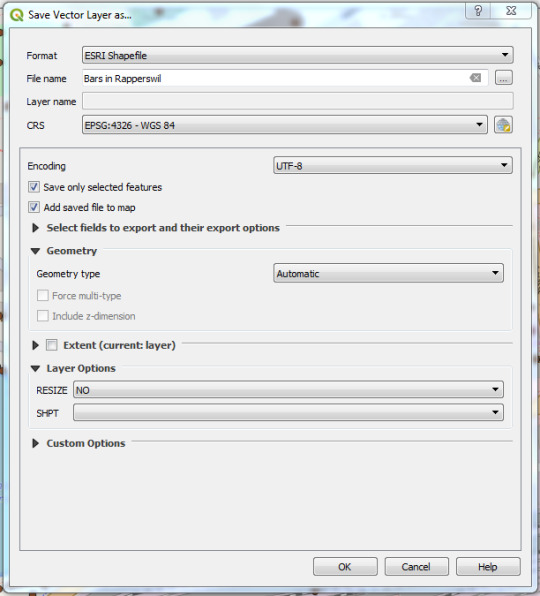
Figure 5. Export selected points.

Import OSM with QGIS-Plugin QuickOSM

You can also import the data into QGIS directly from OSM, using the QuickOSM plugin. If you haven't installed it already you can do so under Plugins > Manage and Install Plugins. Where you can search for QuickOSM and install it.

Figure 6. Installing QuickOSM.

After the installation you open the pluging in a new window under Vector > QuickOSM. Under Quick query you can create a simple query, which will be handled by Overpass-API. 

Under the ledge Query and under Parameters you can select the different instances of Overpass-API. You can for example replace the preset Overpass-Instance with http://overpass-turbo.osm.ch/.

You can also create more difficult queries by hand using OverpassQL. You can find more information about OverpassQl, or overpass-turbo on https://wiki.openstreetmap.org/wiki/Overpass_API/Overpass_QL and on http://osmlab.github.io/learnoverpass/en/.

Figure 7. Create query with the QuickOSM Plugin.

The result of the queries will be saved directly in QGIS as a new layer.

[geometalab]

Creating a Thematic Online-Map using uMap

The goal of this blog post is to show how one can create a thematic online map using uMap with thematic data coming either from OpenStreetMap directly or from a layer added “by hand”.

This instruction can be read in a row, but typically one follows the instructions and then jumps directly to another chapter where the instruction continues based on given requirements and eventually existing data.

Figure 1 shows a decision tree which has to be read from the root top. Depending on the questions the tree finally points to chapters.

Figure 1: Decision tree (see larger image) containing the chapter numbers with instructions on how to include (own) geodata in uMap (from OpenStreetMap).

1. Integrate geodata in uMap

To begin with, search in OpenStreetMap (OSM) for the geodata you want to integrate in uMap. What we actually are looking for is the tags, the key-value-pairs, like “tourism=zoo” for zoo. Consider these web tools to look for these OSM tags: taginfo, OpenStreetMap Wiki and tagfinder.

If you can’t find the tags (meaning the geodata) you need in OpenStreetMap, take a look at the next chapter 2. Otherwise, skip chapters 2 and 3 and continue with chapter 4.

2. Data not available in OpenStreetMap

If the data you want to use - in our case for uMap - is not available in OpenStreetMap, you have the following choices:

Goto chapter 2.1 “Capture data manually in uMap“ if the amount of data is not too big.

Goto chapter 2.2 “Capture data in another tool“ if you want to gather your data in text format.

Goto chapter 2.3 “Capture data in OpenStreetMap“ if the data is suitable for OpenStreetMap and you want to include them.

Goto chapter 3 “Data available as external data / data source“ if the data already exists in a geodata-format that is supported by uMap.

2.1 Capture data manually in uMap

You can capture data manually in uMap. While doing so, it does matter how much geodata you want to record: if it’s too much the browser can slow down quickly or even stop working because of lack of memory. If there are only a few records - i.e. less than 5000 - take a look e.g. at OpenSchoolMaps and the topic “Create a situation plan with uMap” (”Mit  uMap  einen Lageplan  erstellen”) there. If the data you’re going to enter in uMap fits to OpenStreetMap, consider capturing sharing it there, since this is the most sustainable way: see chapter 2.3.

2.2 Capture data in another tool

Instead of capturing the data in uMap you can also use another tool, like the website geojson.io or QGIS desktop.

If you’d like to do it with QGIS, look at “Management and capturing of Geodata“ (”Verwaltung  und  Erfassung  von  Geodaten”) in the QGIS section on OpenSchoolMaps. Geojson.io is a simple online geodata editor which allows you to edit points, lines, and polygons, manage attributes and exchange this with GeoJSON or other well-known formats.

After you’ve captured your geodata, either copy the data to the clipboard and insert it in uMap (by clicking 'import data), or save and export it as a GeoJSON file.

For importing geodata into uMap goto to chapter 3.

Note

Make sure your data has one of the following file extensions: GeoJSON, CSV, GPX, KML, OSM (XML), GeoRSS, uMap. We recommend to import data using GeoJSON. GeoJSON is a human-readable format which e.g. supports attribute name lengths greater than 10 as opposite to Shapefiles. If you decide to go for CSV make sure you have a column for lat and lon. All other columns are imported as attributes. Under ‘Choose the format of the data to import’ (figure 2) you have to choose the format of your file. Click the button ‘Import’ and all your data will be imported in uMap.

Figure 2: Example on how to paste and import a GeoJSON data in uMap.

2.3 Capture data in OpenStreetMap

Another possibility is that you capture the data directly in OpenStreetMap e.g. using the built-in editor (called “iD”) which is the default when you click on ‘Edit’ on the website. The advantage of curating the data in OpenStreetMap is, that the data can be used in different services and is accessible for everyone. Note that - once entered - the data is not available right away, because it must be distributed and processed first among the OpenStreetMap infrastructure.

The worksheet “Edit OpenStreetMap” (”OpenStreetMap bearbeiten”) on OpenSchoolMaps explains how to record the data in OpenStreetMap. If the data were successfully added to OpenStreetMap you can jump to chapter 4.

Note

Make sure the data is suitable for OpenStreetMap. That means only objective/verifiable facts are captured, no subjective nor personal data, and all data must be compliant to the OBbL licence.

3. Data available as external data / data source

If the required data is available as an external file or data source, you can it import into uMap. In uMap just navigate to ‘Import Data‘ and click on the ‘Browse…’-button. Choose your local file and confirm with ‘Open’.

Under ‘Choose the format of the data to import’ you have to choose the format of your file.

Click the button ‘Import‘ and all your data will be imported in uMap.

Note

As mentioned before, prefer the GeoJSON format if possible. Make sure that the data complies with the OBbL licence.

4. Data available in OpenStreetMap

4.1 A snapshot from the OSM data

To import the current status of the data into uMap you can conventiently use the webservice Overpass-Turbo (or Overpass-Turbo swiss edition). With the wizard tool there you can search for certain tags in OpenStreetMap. If you’re happy with the results you can export the data as GeoJSON by clicking the button ‘Export’.

4.2 Keeping data up to date

If you want to keep your data in uMap up to date, it’s very similar to the process described in the preceding section. Just open Overpass-Turbo as instructed before, and do some searching with the wizard, for example „tourism=zoo“. Now choose menu ‘Export’, open ‘Query’ section, then click on ‘placeholders/copy’ below ‘convert to OverpassQL’ (see figure 3).

Figure 3: Export Query from Overpass-Turbo.

By clicking on ‘copy’ you now have an URL in your clipboard. Go to the uMap view, edit the actual layer (or create a new one) by clicking on the pen symbol under ‘Manage layers’ (figure 4).

Figure 4: Editing a Layer in uMap.

Open ‘Remote Data’ from the ‘Edit’ menu and insert the copied URL into the text field URL (figure 5). As format select ‘osm’ and activate the button ‘Dynamic’ (see ‘ON’ in figure 5).

Figure 5: Entering a remote data in uMap.

Now your map contents will always be up to date when a change is made in the OpenStreetMap data, since it will request the data using the Overpass service. On the other hand, using an external service like this involves a dependency and the response time won’t be as fast compared to data coming directly from uMap.

Under ‘From zoom‘ (figure 5) you can define the minimum zoom if you like. This is the zoom level where the map data is being displayed. But that’s only necessary if uMap has a lot of data to display.

If the data clutters the map visually, one can cluster a layer by configuring uMap with another dialog (’point cluster’).

5. Conclusion

With a click on the blue ‘Save’ button above right an d the disable editing button the map is finished.

Now, you can share your map with others and/or integrate it to your website as iframe.

APPENDIX: Online Resources

uMap Webapp: https://umap.openstreetmap.fr/

uMap Guide: https://wiki.openstreetmap.org/wiki/UMap/Guide

Overpass: https://wiki.openstreetmap.org/wiki/Overpass_API

OpenSchoolMaps - e-learning material: OpenSchoolMaps.org

[geometalab]

QGIS Tips & Tricks: Vector Tiles (VT) Reader plugin for QGIS 3

Previously, we have talked about basemaps in QGIS and explained how to add them to QGIS 3. Then, we presented the QuickMapServices plugin which makes it easy to add raster-based tile map services (TMS) as basemaps to a QGIS project. This time, we are going to talk about another QGIS 3 plugin, Vector Tiles Reader (VT Reader), which pulls vector tiles into QGIS and which is maintained by Martin Boos and the Geometa Lab at HSR.

Now, to make sense of the QGIS VT Reader and its capabilities, one needs to understand the potential of Vector Tiles and its difference to TMS. If vector tiles technology is new to you, we recommend reading an earlier blog post. Despite the fact that the technology is still changing and that there exists not yet a specification from OGC yet, the potential and capabilities of Vector Tiles arguably outweight the raster-based TMS (and others) in many aspects, like performance, adaptability of style and attribute appearance. 

Figure 1: OpenMapTiles of Zug region, Switzerland (Credits to Klokan Technologies Zug).

The QGIS VT Reader uses and reads Mapbox Vector Tiles (MVT) from Vector Tile servers, MBTiles files, and from directories. All sources deliver tiled Protobuf files (pbf). The VT Reader then decodes them into a GeoJSON layer which is then added to the current QGIS project. The plugin can also generate a QGIS styling from a Mapbox GL JSON style, which is converted on-the-fly the first time the source is added to QGIS. More information and a help can be found on the repository of the plugin.

Figure 2: QGIS VT Reader plugin dialog connected to OpenMapTiles with “Base map defaults” set (Credits of OpenMapTiles to Klokan Technologies Zug).

Using the QGIS VT Reader

Because its a Python plugin, installing the VT Reader simply means heading over to QGIS menu “Plugins”.

For those who want to install it manually this is the procedure: Either follow the steps on the develop branch of its GitHub repository, or clone the folder and move it into your QGIS 3 plugin directory. For Windows users the directory is at: “%appdata%\QGIS\QGIS3\profiles\default\python\plugins\“.

Now that you have the plugin set up, this is how to use it:

Look out for the VT Reader symbol (shown above).

or go to either to Layer -> Add Layer -> Add Vector Tiles Layer... or to Vector -> Vector Tiles Reader -> Add Vector Tiles Layer...

Under Connections, select the pre-installed OpenMapTiles server - or create your own connection.

Once connected successfully, you usually just keep the defaults (e.g. Base Map) and click Add (all) to load the vector tiles into your QGIS project.

The plugin is intuitive to use and you may want to add your own connection for other vector tile servers that are not pre-installed. More information can be found on the QGIS VT Reader help page.

Note that only those vector tiles providers which come with a predefined style provide a visually appealing base map out-of-the-box. If there is no style provided, QGIS chooses the styles randomly and leaves up to the user to style the layers.

Figure 3: OpenMapTiles with accompanying style showing Rapperswil area (Switzerland) at zoom level ~12 (Credits of OpenMapTiles to Klokan Technologies Zug).

Credits go to Martin Boos (developer of the Vector Tiles Reader plugin) and all the testers, to Petr Pridal (Klokan Technologies Zug) for providing the plugin icon and free access to OpenMapTiles, and as well to the other free vector tiles providers, Nextzen and Mapcat.

[geometalab]

QGIS Tips & Tricks: QGIS 3 Plugin QuickMapServices

We talked about basemaps in another post here, detailing how you can configure QGIS 3 to add your own background maps. With the release of QuickMapServices (QMS) plugin for QGIS 3, this process no longer has to be tedious.

QMS is an “open catalog of geodata sources and a way to add them to your GIS in one click“ - as described by the QMS webpage from NextGIS. This means you can choose from an open and online source of web based map services, and then using the plugin, very simply (search and) select it, and then add it into your QGIS project in just a few clicks.

Simple enough, right? QMS supports four types of map services, namely:

Tile Map Service (TMS)

Web Map Service (WMS) Web

Feature Service (WFS)

GeoJSON file format.

It may be a little daunting at first to learn the differences between these types, but unless you are trying to custom add services not in QMS’s catalog, you should be fine with just knowing that there are different services. TMS is the one which we covered in the previous post, with the zxy format that gives the zoom levels as well as coordinates. We will also explain how to add your own map services.

Figure 1: QuickMapServices menu.

How to use QMS?

1. First and foremost you have to install the QMS plugin. Click on Manage and Install Plugins from the menu toolbar at the top of QGIS. Next, search for QuickMapServices and make sure that it is installed and the checkbox beside it is ticked.

2. Now that you have QMS installed you should see that some new icons appear on your toolbar. 

The QuickMapServices icon has already pre-added map services where you can click to just add the map service’s map layer into your project. 

3. On the right of the QuickMapServices icon is the Search QMS icon. When you click it, a toolbox appears on the right. You can search for a map service you would like to use and then click Add to add it into your project. 

And that’s it. QMS’s website also has a help page to get you started on using it, you can find it here.

Continue reading if you are interested in adding your own map service.

How to add map services in QMS?

If you ever need to use a map service that is not already on QMS’s catalog, which is actually rather unlikely, you may want to add it yourself. As mentioned earlier, there are four types of map services that you can add into the QMS plugin and subsequently your QGIS project. 

1. To begin, you need to know what type of map service you are trying to add, and if it belongs to one of the map services that QMS supports. It also helps to know what are the features of each different type of the map services. Some information can be found on QMS’s webpage here.

2. As a rule of thumb, all the different map services naturally have different formats and provide different sorts of mapping data/image. TMS provides tiled images in the zxy format, which is what we covered in the previous blog post. WMS provides untiled imagery, and the format in their request link contains keywords like “wms” or “WMSserver”. WFS provides vector data, and like WMS, their request link should contain words like “wfs” or “WFSserver”. GeoJSON is essentially just a JSON file, which is a single file with data that can be hosted anywhere and requested, as long as it’s in valid GeoJSON format.

3. Next, you would need a working URL that is in the above mentioend format according to the type of map service. You can read more about it in the link provided in point 1. If you have read our previous post on adding basemaps, the format we used were for tile maps, so if you meddled with the code in the previous post, you might have a better idea of how to add map services into QMS.

4. To add your own map service into QMS, you have to register or sign in into your QMS account. Next, click Add Service and fill in a form to add your map service. And that’s it. Once the service you added is uploaded into QMS’s database and server, you can now search for your web service on the QGIS client and add it into your projects.

In this blog post we have chosen QMS in order to easily get base maps for QGIS 3. There are another plugins to be mentioned, like the OpenLayers plugin and the Vector Tiles Reader plugin. The latter is maintained by the Geometa Lab HSR and will be covered in a following post. Stay tuned!

[geometalab]

QGIS Tips & Tricks: Basemaps for QGIS 3

In anticipation to our workshop at GeoPython Conference 2018 (see also this post), we will be releasing a series of blog posts titled "QGIS Tips and Tricks", that make QGIS even easier and better to use. Today’s post talks about what basemaps are and teaches you how to pull basemaps from online sources with out-of-the-box means without any other plugins. Before we progress, credits for the source code of the basemaps pulling goes to Klas Karlsson (see his original blog and video).

You may have stumbled upon the term “basemaps” before, and wondered what exactly are basemaps? Basemaps, are just simply put: a map layer that provides users with the context of a map in order to give him orienation in the geospace. It is a collection of GIS data, imagery, and or other information that is in the background of a map. As you may already figured out, a map itself is not enough to portray all information of an area, and users tend to only require certain aspects of such information. For example, a navigating midshipman would not be concerned with the population data and similar census of a location, while a biodiversity researcher would probably not be interested in the infrastructure data of an area.

Adding own base map providers

On certain GIS software, like QGIS, there exists built-in functions where you can pull existing datasets from online sources as basemaps.

In addition there are also plugins which facilitate access to existing base map providers, like OpenLayers, QuickMapServices and Vector Tiles Reader. With the new release of QGIS 3, plugin authors had to port plugin scripts from QGIS 2 to QGIS 3. The migration of these plugins took a while due to changes from QGIS 3 upgrading to Python 3.6 from Python 2.x. As such, many plugins, like OpenLayers and QuickMapServices were not available in QGIS 3.0 (they were not at the point of writing, but QMS is now available on QGIS 3), which can limit the available basemaps for a user to use. We will dedicate two separate blog posts, one about QuickMapServices and one about Vector Tiles Reader.

The following details how you can achieve this by using a custom script.

OpenStreetMap basemap used as a layer on QGIS 3.0

Here we show you how we can add our own basemap using the XYZ connections and we also show you step-by-step (based on Klas Karlsson’s YouTube video here) on how to do it.

Although this post might seem to be obsolete as the plugins are now working on QGIS 3, it shows how pulling basemaps from providers work and how we can customize it with our own maps. This general know-how of the format and parameters used to pull maps from online providers is also very useful and serves as a good introduction as the next 2 blog posts would be about something similar, using QuickMapServices and Vector Tiles Reader to pull maps from online providers. 

Let’s now explore how we can pull basemaps from online sources. Currently, this post only covers raster tiled basemaps to be pulled, but a blogpost about pulling Vector Tiles is already in the midst of being prepared, so watch this space for future updates of our plugin!

To add basemaps from online sources with a custom script:

1. You have to write a script that adds online sources to your QGIS browser. Luckily for us, Karlsson has written a custom script here that simplifies the process and all you have to do is to save the script

2. Open up the Python Console by navigating on the menu: Plugins -> Python Console or pressing Alt + Ctrl + P on the keyboard

3. Next, click on Show Editor on the Console, and then click on Open Script on the Editor tab, and then navigate to the script you saved previously

4. The script will then appear on the tab of scripts, as qgis_basemaps.py, and all you have to do is to run it for the basemaps to be added onto the QGIS Browser tab

5. Last but not least, just drag the basemaps you want to use into the project tab to display it

Optional: This step teaches you how to add basemaps from your own sources

To add your own sources, you require these parameters: [sourcetype, title, authconfig, password, referrer, url, username, zmax, zmin]. Once you have these, you just need to add a new line in the qgis_basemaps.py script below the list of Sources. 

In the new line, type:

sources.append([sourcetype, title, authconfig, password, referrer, url, username, zmax, zmin])

An example from Karl’s script:

sources.append(["connections-xyz","OpenStreetMap Standard", "", "", "OpenStreetMap contributors, CC-BY-SA", "http://tile.openstreetmap.org/%7Bz%7D/%7Bx%7D/%7By%7D.png", "", "19", "0"])

Once that is done, save the script, and then run it again. Your sources should now be added and the Browser layer of QGIS will now be updated to display the basemaps you wanted to add.

We at the Geometa Lab decided to add more basemaps into Karlsson’s script for our personal use. You are free to use our edited code as well, and you can find it here. List of maps we added:

OSM Swiss (Switzerland only), in standard style, and LV95 and LV03

OSM Swiss, Standard Style

OSM Swiss, Swiss Style

ÖPVN (aka OpenBusMap) Karte Public Transport Map

OpenCycleMap by Thunderforest

Thunderforest Transport Map

Thunderforest Landscape Map

OSM Sweden (Hydda Full)

OSM DE Mapnik

Once again, credits go to Klas Karlsson for the original source code and the respective websites for the basemaps.

[geometalab]

Geometa Lab HSR at GeoPython Conference 2018!

On the 07-09th of May 2018, the University FHNW in Muttenz near Basel will be organizing the GeoPython Conference (see webpage) following the success of the ones held in 2016 and 2017. And we at the Geometa Lab HSR will be there again to present a workshop about geospatial data analysis, as well as the programming language we all love - Python! Our workshop is titled "QGIS Processing Framework: Automating Tasks with Python". It will be held on May 07 at 13:30 (see program details).

In a nutshell, the workshop seeks to teach participants basic literacy in the Processing framework of QGIS which includes a Graphical Modeler. This framework consists of native (predefined) and custom functions to make your spatial analysis tasks more productive and easier to conduct, and to automate otherwise repetitive and tedious geospataial analytical tasks.

The workshop will start with self introductions, and then makes sure that participants have the right version of QGIS 3, which is a rather new and big update to previous iterations. Help with setting up and installing QGIS would also be administered if required. After that, we kick off the actual workshop by introducing QGIS - about QGIS, how it came about, its pros and cons, future works and more.

Once participants are warmed up to the concepts behind QGIS, we then talk about how QGIS can be linked to Python, through PyQGIS, its native built in Python console. We will continue with a quick run-through of its capabilities, from performing basic Pythonic equations to high leveled Pythonic scripts, as well as methods native to the QGIS Qt library. We will also explain how the implementation of the PyQGIS is achieved with the Processing framework as well as how it allows us to create custom scripts, among other nifty tools, like the Graphical Modeler and Plugins, via the Processing Toolbox feature.

And now that we have piqued your interest, we move on to the main event. We will show you the Graphical Modeler, Plugin and Processing Script in action to demonstrate the prowess of QGIS and Python, before letting you get down and dirty by trying out our bite sized hands on exercises created specially to help you through this crash course. Finally, once we have all become considerably versed with automating geodata analysis tasks with scripts, we wrap up and conclude our 2 hours workshop and hopefully, you'd be positively reinforced and motivated to learn further on your own!

Keep 07th to 09th May free - because we sure hope you are looking forward to joining us as much as we are to meet you! For any questions that you may have, do not hesitate to contact us.

Credits: http://2018.geopython.net/

[geometalab]

Vector Tiles – The Web Mapping Technology of the Future?

Vector tiles have geographic data which are optimized for graphic, partial display within certain levels of zoom. They are comparable to raster tiles, known through webmap applications, but they contain pre-processed raw data with vector geometries and attributes.

The two-dimensional vector tiles became famous from the company Mapbox around 2014. Back then, the “Mapbox Vector tiles” specification was published. Mapbox itself uses the web Mercator projection, and a continuous 256x256px tile scheme. Moreover, vector tiles are not limited to a certain map projection, they can also be defined in different tile sizes and schemes.

Vector tiles are transferred and exchanged like raster tiles. The transfer happens either through compressed (zipped) form, via interface (for example: https://example.com/17/65535/43602.pbf or *.mvt), or through a single, packed file (mbtiles-format and others). Once received by the client, the vector tiles are converted into a map. This “rendering” all happens within a GPU-Coprocessor, making the presentation especially smooth.

Meanwhile, there are different applications which are able to display Vector tiles, ranging from mobile apps, to web GIS, to desktop GIS. The styles are dependent on the client, which decides which style is displayed. Mapbox has published a “Styling Language” for their client software and has developed different map styles (see Mapbox article). Like Mapbox, every application has its own styles as they rely on a client-specific styling Language and certain specific tile data. The Vector tiles are specified by almost all providers (Google, Apple, Mapbox, Mapzen, Esri and others) and viewed as part of their interface; those at OpenMapTiles can even be downloaded. Mapbox and ArcGIS Pro offer special editors to adjust map styles; with QGIS, that is done via the normal style editor.

Figure 1: The principle of generating vector tiles. Source: Gaffuri (2012).

With the respective software, Vector tiles can be generated by anyone (see Awesome Vector Tiles). During creation, the original geodata is filtered by zoom level and also geometrically simplified. The result is an optimized dataset that gets more detailed with each level. Finally, the objects are tiled and coded (Protocol Buffers, PBF), see figure 1. An interesting point to note is that objects, like labels, streets, and areas inside the tile data can exceed the limits of the tile. The client software can decide whether those objects will be clipped or left whole.

The level of detail of the vector data is so high, that it often can’t be generated up to the highest level. If one zooms further than that, the data is then displayed bigger than it actually is (overzooming). The fact that the highest level is capped makes it easier for vector tile producing software, especially when large areas have to be pre-processed.

Efficient for transfer: The data packages are much smaller than non-tiled ones, because only tiles within the specified area are transmitted in the first place, if the transmission is necessary (some providers transfer, as mentioned, no new data from zoom level 14 onwards.)

Compact: Compared to raster tiles (e.g. OGC WMTS), vector tiles take considerably lesser time to process as a single vector tile contains lesser bytes (<5kB).

Efficient for servers: A webserver is enough for the distribution of the vector data, just as it is with raster tiles, and data can be cached easily. No special GIS servers (as opposed to OGC WMS) are required, to cut out a certain map area.

Interactive and informative: In spite of the compactness of vector tiles, it’s possible to query the attributes of the map objects (see figure 2) and to change, for example, the language of the map objects.

Flexible and adaptive: The map can be rotated and tilted by the user, all while the labels stay right-side up. And it has, given the right know-how, become easier to choose or make a map visualization.

On the other hand, there are of course, disadvantages and limitations: Vector tiles, for example, almost always lose some data due to filtering, generalization, line and polygon clipping, and more. This makes analyzing the data more difficult thus, it is not suited for being edited and then put back into the original dataset. 

Figure 2: Map graphic with a “window”, which displays the content (JSON) of a vector tile. Source: Mapzen.

Obviously, the vector tiles technology is still unfinished. That explains why there is no standardization of OGC/ISO (cf. OGC) yet. The advantages of vector tiles are overwhelming and in web GIS, the usage as background map is given (see also this article from Carto). There is also potential in using vector tiles as an exchange format or for offline mobile applications. The future can only show how far vector tiles can get.

Are you interested in learning more about those technologies? We offer further education (cf. our agenda), counsel and other services. Contact: Prof. Stefan Keller.

This article was first published in german and french with the title "SOGI FG4: GIS-Technologie-News" in the SOGI Infoblatt / OSIG Bulletin d’information Nr. 4, 2017. Thanks to Markus Schenardi and the SOGI Fachgruppe GIS Technologie.

[geometalab]

Vector tiles – la technologie des cartes Web de demain?

Les Vector tiles («tuiles ou tesselles vectorielles») contiennent des données géographiques optimisées en vue d’une représentation graphique par extraits, au sein de plages de zoom bien définies. On peut les comparer aux tuiles ou tesselles tramées (raster) bien connues des applications de cartes Web, mais elles comprennent des données brutes prétraitées avec des géométries et des attributs de vecteurs.

Les Vector tiles bidimensionnelles doivent leur notoriété à Mapbox qui les a fait connaître en 2014 en publiant la spécification «Mapbox Vector Tiles». Cette société utilise la projection de Mercator Web et une mosaïque régulière basée sur des tesselles de 256x256 pixels. Les Vector tiles ne sont toutefois pas limitées à une projection cartographique particulière et peuvent être définies pour un grand nombre de dimensions et de modèles de mosaïques.

Les Vector tiles sont transmises et échangées comme les tesselles tramées. La transmission s’effectue sous une forme compressée (zippée) via une interface – ex. : https://example.com/17/65535/43602.pbf resp. *.mvt – ou par le biais d’un fichier unique compressé (notamment au format mbtiles). Au sein du client, les Vector tiles – auxquelles des instructions de représentation sont jointes – sont converties en une représentation cartographique. Cette conversion («rendering») est de préférence réalisée à l’aide d’un coprocesseur GPU, ce qui rend la représentation particulièrement fluide.

Aujourd’hui, les clients les plus divers peuvent représenter des Vector tiles, de l’appli pour mobile au SIG de bureau en passant par les SIG Web. Les représentations cartographiques (styles en anglais) dépendent du client puisque c’est lui qui décide en cette matière. Mapbox a publié un «Styling Language» pour son logiciel client et a ainsi conçu des styles de cartes très variés (cf. Mapbox article ). A l’instar de Mapbox, chaque fournisseur dispose de ses propres styles de cartes, chacun de ces derniers se fondant sur un «Styling Language» spécifique au client et sur des données de mosaïque bien précises. Les tesselles vectorielles sont prédéfinies par presque tous les fournisseurs – dont Google, Apple, Mapbox, Mapzen et Esri – qui considèrent qu’elles font partie intégrante de leur interface ; OpenMapTiles permet même de les télécharger. Mapbox et ArcGIS Pro proposent des éditeurs spécifiques pour adapter les styles de cartes ; c’est l’éditeur de style normal qui sert à cela dans le cas de QGIS.

Figure 1 : principe de génération de Vector tiles. Source : Gaffuri (2012).

On peut générer les Vector tiles soi-même si l’on dispose d’un logiciel approprié (cf. page web Awesome Vector Tiles ). Lors de la génération, les géodonnées originales sont filtrées en fonction du niveau de zoom avant de subir une simplification géométrique. Il en résulte un jeu de données optimisé, de plus en plus détaillé d’un niveau de zoom au suivant. Les objets sont enfin subdivisés en tesselles (tiling) et codés (Protocol Buffers, PBF) ; cf. figure 1. Il est intéressant de noter ici que des objets tels que des écritures, des routes et des surfaces peuvent dépasser les limites des tesselles dans la mosaïque des données. Le logiciel client peut alors décider si ces objets doivent être détourés ou non (clipping).

Les données vectorielles sont tellement détaillées qu’elles n’ont bien souvent pas besoin d’être générées jusqu’au niveau maximal. Si l’on continue à zoomer, les données vectorielles sont tout simplement agrandies («over-zooming»). Cette limitation à un niveau maximal prédéfini facilite notamment la tâche des fournisseurs de Vector tiles, principalement lorsque des zones géographiques d’une certaine ampleur doivent être prétraitées.

Les Vector tiles présentent plusieurs avantages dans l’optique de la visualisation de cartes :

Efficaces pour la transmission : les paquets de données sont petits par rapport à des données vectorielles non mosaïquées, car seules les tesselles incluses dans l’extrait défini sont transmises – pour autant qu’une transmission soit effectivement requise (comme indiqué, certains fournisseurs ne transmettent plus de nouvelles données à partir d’un certain niveau de zoom, le niveau 14 par exemple).

Compactes : en comparaison de tesselles tramées (par exemple OGC WMTS) aussi, on observe un gain de vitesse, les tesselles vectorielles contenant généralement moins d’octets (< 5 Ko).

Efficaces pour le serveur : un serveur Web est suffisant pour la distribution des données vectorielles – comme pour les tesselles tramées – et les données peuvent simplement être enregistrées dans la mémoire cache. Aucun serveur SIG particulier (ce qui est par exemple le cas d’OGC WMS) n’est requis pour découper un extrait de carte.

Interactives et informatives: en dépit de la compacité des tesselles vectorielles, le client accepte des requêtes pouvant porter sur les attributs des objets de la carte (cf. figure 2) et il est par exemple possible de modifier la langue associée à ces objets.

Flexibles et adaptables : le client peut procéder à une rotation de la carte, les écritures pouvant rester horizontales. Et il est devenu plus simple – si l’on dispose du savoir-faire requis - de sélectionner la représentation de la carte ou de l’organiser soi-même.

Les Vector tiles ne sont toutefois pas exemptes d’inconvénients ou de limitations : ainsi, on enregistre presque toujours des pertes par rapport aux données originales (en raison notamment du filtrage et de la généralisation, d’arrondis de coordonnées / du codage, du détourage de lignes et de polygones). Elles sont donc plus difficiles à analyser et ne conviennent pas pour une édition suivie d’un retour au jeu de données original.

Figure 2 : représentation cartographique incluant une «fenêtre» présentant le contenu (JSON) d’une tesselle vectorielle. Source : Mapzen.

De toute évidence, la technologie des Vector tiles est encore en pleine évolution (métadonnées, 3D, etc.), ce qui explique aussi l’absence de standardisation/normalisation de la part d’OGC/ISO pour l’heure (cf. OGC). Les avantages des Vector tiles sont toutefois séduisants et les applications comme carte d’arrière-plan sont toutes trouvées dans le domaine des SIG Web (voire aussi cette article an anglais). Leur utilisation comme format d’échange ou pour des applications mobiles hors ligne semble également riche de promesses. Jusqu’où les Vector tiles iront-elles? C’est l’avenir qui nous le dira.

Souhaitez-vous savoir plus sur ces technologies? Nous offrons des formations avancées (voir le programme), des conseils et certains services. Contact: Prof. Stefan Keller.

Cet article a été publié pour la première fois sous le titre "SOGI FG4: GIS Technology News" dans l’ OSIG Bulletin d'information n ° 4, 2017. Merci à Markus Schenardi et à la section OSIG Technology SIG.

[geometalab]

Vector Tiles – Die Webkarten-Technologie der Zukunft?

Vector Tiles sind "Vektor-Kacheln" mit geografischen Daten, die optimiert sind für die grafische, ausschnittweise Darstellung innerhalb bestimmter Zoomstufen. Sie sind vergleichbar mit den aus Webkarten-Anwendungen bekannten Raster-Kacheln, enthalten jedoch vorverarbeitete Rohdaten mit Vektor-Geometrien und Attributen.

Die zweidimensionalen Vector Tiles sind um etwa 2014 durch die Firma Mapbox bekannt geworden. Damals wurde die "Mapbox Vector Tiles"-Spezifikation publiziert. Mapbox selber verwendet die Web Mercator-Projektion und ein regelmässiges Kachel-Schema auf Basis von 256x256 Pixel. Die Vector Tiles sind jedoch nicht auf eine bestimmte Kartenprojektion eingeschränkt und können in unterschiedlichen Kachel-Grössen und Kachel-Schematas definiert sein.

Vector Tiles werden wie Raster-Kacheln übermittelt und ausgetauscht. Die Übermittlung geschieht entweder in komprimierter Form (ge-zipped) über eine Schnittstelle – zum Beispiel https://example.com/17/65535/43602.pbf bzw. *.mvt – oder mittels einer einzelnen, gepackten Datei (u.a. mbtiles-Format). Im Client angekommen, werden die Vector Tiles - zusammen mit Darstellungsanweisungen - in eine Kartengrafik umgewandelt. Dieses "Rendering" geschieht vorzugsweise mit einem GPU-Koprozessor, was die Darstellung besonders flüssig macht.

Inzwischen gibt es unterschiedlichste Clients, die Vector Tiles darstellen können, vom Mobile App über Web-GIS bis zum Desktop-GIS. Die Kartendarstellungen (engl. styles) sind vom Client abhängig und er entscheidet, welcher Style angezeigt wird. Mapbox hat für ihre Client-Software eine "Styling Language" publiziert und hat damit verschiedenste Kartenstile entworfen (vgl. Mapbox Artikel). Wie Mapbox hat jeder Anbieter seine eigenen Kartenstile, denn jeder Style beruht auf einer Client-spezifischen Styling Language und auf bestimmten Kacheldaten. Die Vektorkacheln werden von praktisch allen Anbietern – u.a. Google, Apple, Mapbox, Mapzen und Esri – vorgegeben und als Bestandteil ihrer Schnittstelle betrachtet; bei OpenMapTiles kann man sie sogar herunterladen. Mapbox und ArcGIS Pro bieten spezielle Editoren an, um Kartenstile anzupassen; bei QGIS geht das über den normalen Stileditor.

Abbildung 1: Erzeugungsprinzip von Vector Tiles. Quelle: Gaffuri (2012).

Mit entsprechender Software können die Vector Tiles auch selber generiert werden (siehe die Webseite “Awesome Vector Tiles“). Bei der Erzeugung werden die originalen Geodaten je nach Zoomstufe zuerst gefiltert und dann geometrisch vereinfacht. Dadurch entsteht ein optimierter Datensatz, der von Stufe zu Stufe detaillierter wird. Schliesslich werden die Objekte gekachelt (tiling) und codiert (Protocol Buffers, PBF); siehe Abbildung 1. Interessant an dieser Stelle ist, dass Objekte wie Beschriftungen, Strassen und Flächen in den Kacheldaten über die Kachelgrenzen hinausragen können. Die Client-Software kann dann entscheiden ob die Objekte abgeschnitten werden oder nicht (clipping).

Der Detaillierungsgrad der Vektordaten ist so gut, dass sie oft nicht bis zur höchsten Stufe generiert werden. Zoomt man weiter herein, werden die Vektordaten vergrössert dargestellt ("over-zooming"). Diese Beschränkung auf eine bestimmte Höchststufe erleichtert u.a. die Arbeit von Vector Tile-Providern, vor allem wenn grössere geografische Bereiche vorverarbeitet werden müssen.

Vector Tiles haben mit Blick auf die Kartenvisualisierung verschiedene Vorteile:

Effizient für die Übertragung: Gegenüber nicht gekachelten Vektordaten sind die Datenpakete klein, denn es werden nur die Kacheln innerhalb des Ausschnitts übertragen - falls eine Übertragung überhaupt nötig ist (einige Provider übermitteln wie erwähnt z.B. ab Zoomstufe 14 keine neuen Daten).

Kompakt: Auch im Vergleich zu Rasterkacheln (z.B. OGC WMTS) ergibt sich ein Geschwindigkeitsvorteil, da Vektorkacheln meist weniger Bytes enthalten (< 5 KB).

Effizient für den Server: Es genügt ein Webserver für die Verteilung der Vektordaten wie bei Raster-Kacheln - und die Daten können einfach zwischengespeichert (ge-cached) werden. Es braucht keine besonderen GIS-Server (wie z.B. bei OGC WMS), um einen Kartenausschnitt auszuschneiden.

Interaktiv und informativ: Trotz der Kompaktheit der Vektorkacheln ist es im Client möglich, die Attribute der Kartenobjekte abzufragen (vgl.  Abbildung 2) und zum Beispiel die Sprache der Kartenobjekte zu wechseln.

Flexibel und adaptiv: Die Karte kann vom Client rotiert und gekippt werden wobei die Beschriftungen horizontal bleiben können. Und es ist – bei entsprechendem Knowhow einfacher geworden, die Kartendarstellung auszuwählen oder selber zu gestalten.

Auf der anderen Seite gibt es auch Nachteile und Einschränkungen: Vector Tiles enthalten beispielsweise fast immer einen Datenverlust gegenüber den Originaldaten (u.a. wegen Filterung und Generalisierung, Koordinatenrundung/Codierung, Line- und Polygon-Clip-ping). Dadurch ist deren Analyse erschwert und sie sind nicht geeignet, editiert und wieder in den Originaldatensatz zurückgeschrieben zu werden.

Abbildung 2: Kartengrafik mit "Fenster", das den Inhalt (JSON) einer Vektorkachel zeigt. Quelle: Mapzen.

Offensichtlich ist die Vector Tiles-Technologie immer noch im Fluss (Metadaten, 3D, etc.). Dies erklärt auch, warum es noch keine Standardisierung von OGC/ISO gibt (vgl. die OGC Website). Die Vorteile der Vector Tiles sind jedoch bestechend und im WebGIS-Bereich sind die Anwendungen als Hintergrundkarte gegeben (siehe auch dieser Artikel (engl.)). Potential besteht auch darin, die Vector Tiles als Austauschformat oder bei mobilen Offline-Anwendungen zu verwenden. Die Zukunft wird zeigen, wie weit sich die Vector Tiles durchsetzen.

Sind Sie interessiert, mehr zu diesen Technologien zu erfahren? Das Geometa Lab bietet Weiterbildung (Agenda), Beratung sowie auch Dienstleistungen an. Kontakt: Prof. Stefan Keller.

Dieser Artikel ist erstmals erschienen unter dem Titel "SOGI FG4: GIS-Technologie-News" im SOGI Infoblatt / OSIG Bulletin d’information Nr. 4, 2017. Dank an Markus Schenardi und an die SOGI Fachgruppe GIS Technologie.

[geometalab]

Easily create appealing web maps using the HTML Image Map Creator plug-in for QGIS

Introduction

Today's Internet allows for a high degree of interactivity, but a simple web map often achieves a better effect on the reader. This is confirmed by Brian Timoney in his blog post entitled "Few Interact With Our Interactive Maps ...". With the "HTML Image Map Creator" plugin for QGIS, an aid is to be presented here in order to easily design such web maps.

QGIS is a desktop software, an open geographic information system for the visualization of geo data. QGIS can be easily extended with so-called plugins, whether as a user or as a programmer. With the "HTML Image Map Creator", a user with QGIS can create a simple web map. He can freely choose which basic map and what information he wants to portray. 

As an example, we created a web map showing where you can rent “Pedalos” (paddleboats) around Lake of Zürich (figure 1). This map is intended for online publications, but can also be used in printed form. 

Figure 1: Map with pedal boats for rent around the Lake of Zurich (Switzerland).The map style "Gray" from Wmflabs serves as the base map. Pedalos (paddleboats) and map data are from the OpenStreetMap project. (Copyright: Geodata © OpenStreetMap contributors ODbL, Kartengrafik © Wmflabs CC-BY-SA).

This map containing markers with labels would ready be ready for printing. For the browser, though, we will add some interactivity (just with little HTML5 code without big Javascript libraries): There you can click on a marker and an "Infobox" opens (figure 2). In our case, this information box contains information consisting of the following fields: "name" (bold), "contact: phone", "website" and "opening_hours". More on that later.

Figure 2. Infobox to a pedal boat rental site after clicking on a marker (blue drop icon).

For our map, we need two "layers": a background for orientation in the form of a basic map and the actual thematic data, which will then be displayed as markers with "label" and/or "infobox". The following describes the creation of the base map and the thematic layer.

Basemap

First, start QGIS. If QGIS is not already installed, you can download it (works on all platforms). Once QGIS has been started, we take care of the base map. The plugin "QuickMapServices" helps us here (see menu Plugin => Manage Plugins...). Once the plugin has been installed, you can access it via the Web menu or by clicking on the corresponding icon (blue, round). For our example, we used the map "MapSurfer OSM Roads Grayscale" (Menu Web => QuickMapServices => MapSurfer.NET). There are also other possibilities such as "OSM Outdoor" or other base map styles.

Thematic layer

Now we want to supplement the QGIS project with the actual thematic data, the rental pedal boats. Ideally, the data is already available. If this is not the case, one must create it. That is what we want to do now. 

With OpenStreetMap (short: OSM), a useful data source is freely available. It contains hundreds of kinds of "Points of Interests" (POIs), such as shops, benches, viewpoints, etc. If the POIs are not already available, you can enter them yourself in OpenStreetMap. This allows the data to be verified and supplemented by others and later be reused.

Pedal boat rental amenities are attributed in OpenStreetMap with "amenity = boat_rental" and "pedalboat_rental = yes", which are supplemented with the fields mentioned above (name, contact:phone, website and opening_hours).How to capture such POIs in OpenStreetMap, can be learned on the Wiki or in this example .

After capturing the data in OpenStreetMap, you can for example use the webapp Overpass Turbo to download the desired data. First, you can use the zoom and pan to narrow the map region - here it’s the Lake of Zurich. The simplest way of fetching the data is to use the built-in wizard. There you can enter a "tag" which you want to filter, here "pedalboat_rental = yes". Once you have fetched the data, you can click on "Export" to download the filtered data in the file format "GeoJSON" (here a GeoJSON example ). After the export, it is recommended to rename the file, for example to “rental-pedalos.geojson”.

The GeoJSON file has to be inserted into QGIS as further preparation, which can be achieved by simple Drag & Drop. Let’s call the layer "rental pedalos". You may have to adjust the coordinate reference system to the data in the lower right corner of QGIS, for example "EPSG: 3857". QGIS provides a nice marker (blue drop icon) for symbolizing dot objects. 

Furthermore, you should note that the labelling in QGIS should be turned off, since the labelling of the POIs is done by the plugin.

Ready to export, but... 

Now the static map is already done! It can be printed and exported with a "Print Screen" or with the built-in QGIS Print Composer (for example in PNG or JPG format). Note that since everything is "packed" into a single raster graphic, the markers are contained in the graphics as well. 

Since the output is a pure raster graphics, it is hardly possible to apply changes later. If you want to customize the labels size or colour with CSS, the HTML Image Map Creator plugin described below comes into play. 

If you want to bring some interactivity (with simple Javascript) into the game with informative infoboxes, then read the following chapter. This is not mandatory and can be skipped.

Compiling information for the infobox (create virtual field) 

The HTML Image Map Creator plugin, whose configuration is explained in the next chapter, expects a single field from the list of all fields / attributes of a layer / table for labels and infoboxes. In the case of the infobox, the content can be formatted in HTML text, including bold text, line breaks, weblinks or bullets. With some skill, QGIS can now combine several fields (attributes) of a table. If necessary, add HTML markup and place the result as text in a so-called "virtual" field.

To add a virtual field to the fields of a layer (such as the rental pedal boats), use the field calculator in QGIS (see figure 3).

Figure 3: An abacus as a symbol of the field calculator in the QGIS toolbar.

In the field calculator dialog (figure 4) you have to activate the checkbox "Create new field" and the checkbox "Create virtual field". Let's call the virtual field "infobox". Then select the data type "Text (string)" in the "Output field type" dropdown. The output field length is set to 255 characters, which means that longer character strings are truncated there. 

In the middle of the field calculator dialog there is a large, empty text field in the "Expression" tab. This is an editor, which expects expressions as text code. Following, you can see the finished expression code, which can be used for our infobox and can be inserted with Copy & Paste in the expression editor (note that this is a single continuous line without line breaks):

'<b>' || "name" || '</b>' || '<br>' || '<br>' || "contact:phone"  || '<br>' ||  coalesce('<a href =' ||  "website"  || '>' ||  "website"  || '</a>', 'No website') || '<br>' ||   coalesce( "opening_hours", 'No opening hours')

Here is a brief explanation of this expression code: 

The HTML tags (here: '<b>', '<a href>' and '<br>') are enclosed with single quotes

The fields / attributes (here: "name" etc.) are enclosed with double quotes 

The HTML tag <b> title </ b> represents "title" in bold 

The HTML tag <br> without closing tag generates a line break

The HTML tag <a href> defines a weblink, which can later be clicked in the browser

|| Connects the string to each other (concatenate) 

Coalesce (x, y) is a built-in function that tests the value "x": if this is "null", "y" is returned instead, here: if the field “website” is null, “No Website” will be returned.

If you would like to learn more about the powerful expression functions in QGIS, these workshop documents are recommended.

Figure 4: Field calculator with the expression that fills the additional virtual field "infobox" with HTML text.

HTML Image Map Creator

Now we are almost ready to create the web map. If desired, a subset of objects can be selected in the QGIS map view, which should appear as a marker on the map later. 

In any case, a suitable layer has to be selected as active layer in QGIS, before the HTML Image Map Creator is selected (here the rental pedal boats layer). Valid layers are vector layers of type Point (Point or Multi-Point) or Surface (Polygon or Multi-Polygon). 

If all these preliminary workings have been done, the plugin can be opened in QGIS via the Web => HTML Image Map Creator => Create map ... menu.

The HTML Image Map Creator consists of a single configuration dialog (see figure 5). In the upper part of the dialog, you will find a short description. Below are the different information and configuration fields, which are explained in more detail in the next section.

Figure 5: Configuration dialog of HTML Image Map Creator in QGIS. 

The configuration dialog

The first field in the dialog is an information field that displays the size of the map view, which means the visible map section in QGIS. These pixel values ​​must be adapted to the layout of the publication - for example 800 pixels wide and 600 pixels high - by leaving the plug-in, adjusting the map view, and then re-opening the plug-in.

The second field "Active layer" is also an information field. It shows the name of the active layer . In addition, the number of objects in the layer is displayed to the right of the text field. This also includes objects outside the map view.

The third field is responsible for naming and selecting the location of the files, which are to be generated. Using the "Browse" button, the user can decide where to save his files and how to name them. All files are saved with the same path. Choose e.g. name “Pedalos-Rental“.

The fourth field is a checkbox and a drop-down list. The checkbox determines whether the object is labelled on the map. The user must select a field of the layer. The label is placed in the middle of the marker.

The fifth field is for label placement. Positive offset values ​​result in a downward displacement, negative offset values result in upward displacement.

The sixth field has to be activated by ticking of a checkbox, just like "Label". It activates the infoboxes in the export. Again, you have to choose a field of the layer. We recommend creating a virtual field in the QGIS field calculator (see above). If you have not already done so, you must leave the plug-in and open it again when the virtual field is ready. 

The seventh field is for infobox placement. Positive offset values ​​result in a downward displacement, negative offset values result in upward displacement.

The eighth and last line shows a "Selected features only" checkbox and a small statistic. The checkbox determines whether only the selected objects are exported. The small statistics shows how many objects were selected in the layer and how many of these objects are within the  map view. 

After the user has filled out all fields, the OK button, which starts the export, can be pressed at the bottom of the dialog.

If the export was successful, the following three files will be created:

Pedalos-Rental.html: includes the HTML5 code (HTML, CSS, Javascript) including the image map data of the POIs. 

Pedalos-Rental.png: is a raster graphics file; It contains the basic map and is called by HTML file. 

Pedalos-Rental.pgw: Is an auxiliary file, which is mainly read by geo information systems to process the map ("Worldfile"). It can be left out in pure publications. 

These files (especially the .png file and the corresponding code section in the .html file) can now be embedded in a separate blog post and adapted if necessary. You can also only use the graphics file Pedalos-Rental.png. 

In any case, it is up to the author to design an informative map by any means available to QGIS. Now, nothing is preventing an informative summer story!

P.S. The HTML Image Map Creator QGIS plugin is open source and has been written in Python. Feedback and other software contributors are welcome!

Figur 6:  A cooldown for the hot summer days: rental pedal boat in the Lake Zurich.

[geometalab]

Einfaches Erstellen von ansprechenden Webkarten mit dem HTML Image Map Creator Plugin für QGIS

Einleitung

Das heutige Internet erlaubt zwar eine hohe Interaktivität, doch erzielt eine schlichte Webkarte oft die bessere Wirkung beim Leser. Dies bestätigt auch Brian Timoney in seinem Blogpost mit dem Titel „Few Interact With Our Interactive Maps...“. Mit dem „HTML Image Map Creator“ Plugin für QGIS soll hier ein Hilfsmittel vorgestellt werden, um solche Webkarten einfach zu entwerfen.

QGIS ist eine Desktopsoftware, ein offenes Geoinformationssystem zur Visualisierung von Geodaten. QGIS kann mit sogenannten Plugins einfach erweitert werden, sei es als Benutzer oder als Programmierer. Mit dem „HTML Image Map Creator“ kann ein Benutzer mit QGIS eine einfache Webkarte erzeugen. Dabei kann der er frei wählen, welche Basiskarte und welche Informationen er darstellen möchte.

Als Beispiel erstellen wir eine Webkarte, die zeigt, wo man Pedalos am Zürichsee mieten kann (Abbildung 1). Diese Karte ist für Online-Publikationen gedacht, lässt sich aber auch im Druck verwenden.

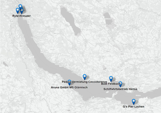
Abbildung 1: Karte mit Pedalos zum Mieten rund um den Zürichsee (Schweiz). Als Basiskarte dient der Kartenstil „Gray“. Pedalos und Kartendaten stammen vom freien Projekt OpenStreetMap (Copyright: Geodaten © OpenStreetMap contributors, Kartengrafik © CC-BY-SA).

Für den Druck reicht diese Karte mit den Markers und mit Beschriftung („Label“). Im Browser ist etwas Interaktivität möglich: Dort kann man auf einen Marker klicken und es öffnet sich eine “Infobox” (Abbildung 2). Diese Infobox enthält in unserem Falle Informationen, die aus den folgenden Feldern zusammengesetzt sind: “name“ (fett), “contact:phone“, “website” und “opening_hours“ (eventuell sind nicht immer Werte vorhanden). Mehr dazu später.

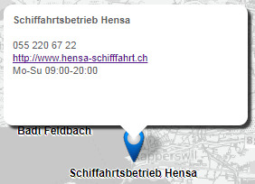
Abbildung 2. Infobox zu einem Pedalo-Standort nach Klick auf einen Marker (blauer Tropfen).

Für unsere Karte benötigen wir zwei "Layers” (Ebenen): einen Hintergrund zur Orientierung in Form einer Basiskarte und die eigentlichen thematischen Daten, die dann als Marker mit „Label“ und/oder „Infobox“ dargestellt werden. Im folgenden wird die Erstellung der Basiskarte und des thematischen Layers erläutert.

Basiskarte

Zuerst starte man QGIS. Falls QGIS noch nicht installiert ist, kann man es herunterladen (funktioniert auf allen Plattformen). Sobald QGIS gestartet ist, kümmern wir uns um die Basiskarte. Diese beschaffen wir mit Hilfe des Plugins „QuickMapServices“ (vgl. Menü Plugin => Manage Plugins...). Sobald das Plugin installiert ist, kann man über das Menü Web oder mit Klick auf das entsprechende Icon (blau, rund) darauf zugreifen. Für unser Beispiel benutzen wir die Karte „MapSurfer OSM Roads Grayscale” (Menü Web => QuickMapServices => MapSurfer.NET). Es gibt auch „OSM Outdoor“ oder andere Basiskarten-Stile.

Thematischer Layer

Nun wollen wir das QGIS-Projekt mit den eigentlichen thematischen Daten, den Miet-Pedalos, ergänzen. Im Idealfall stehen die Daten schon zur Verfügung. Ist dies nicht der Fall, so muss man sie sich selber beschaffen. Dies wollen wir nun tun.

Mit OpenStreetMap (kurz: OSM) steht eine nützliche Datenquelle frei zur Verfügung. Sie enthält hunderte Arten von „Points-of-Interests“ (POIs), wie Shops, Sitzbänke, Aussichtspunkte etc.. Falls die POIs noch nicht vorhanden sind, kann man diese selber in OpenStreetMap eintragen. Damit können die Daten von anderen verifiziert und ergänzt und später wiederverwendet werden.

Pedalo-Vermietungsstellen werden in OpenStreetMap mit „amenity=boat_rental“ und „pedalboat_rental=yes“ attributiert, die mit den oben erwähnten Feldern ergänzt werden (name, contact:phone, website und opening_hours). Wie man solche POIs in OpenStreetMap erfasst, kann man auf dem Wiki oder in diesem Beispiel nachlesen.

Nach der Erfassung der Daten in OpenStreetMap, kann man z.B. mit der Webapp Overpass-Turbo die gewünschten Daten herunterladen. Zuerst kann man mittels Zoom und Pan den Kartenausschnitt eingrenzen – hier auf das Gebiet rund um den Zürichsee. Dann benutzt man am einfachsten den dort eingebauten Wizard. Dort kann man einen „Tag“ eingeben nach dem gefiltert werden soll, hier also „pedalboat_rental=yes“. Hat man die gewünschten Daten ausgewählt, kann man auf „Export“ klicken, um die gefilterten Daten im Dateiformat „GeoJSON“ herunterzuladen (hier ein GeoJSON-Beispiel). Nach dem Export empfiehlt es sich, die Datei umzubenennen, z.B. in Miet-Pedalos.geojson.

Als weitere Vorarbeit muss die GeoJSON-Datei in QGIS eingefügt werden, was mittels einfachem Drag&Drop erreicht werden kann. Nennen wir den Layer „Miet-Pedalos“. Eventuell muss man in QGIS unten rechts das Koordinatenbezugssystem an die Daten anpassen, z.B. auf „EPSG:3857“. QGIS stellt für die Symbolisierung von Punktobjekten einen schönen Marker (blauer Tropfen) zur Verfügung. 

Ausserdem ist zu beachten, dass wir in QGIS die Beschriftung der Objekte ausschalten sollten, da die Beschriftung der POIs durch das Plugin übernommen wird.

Fertig zum Export, aber...

Nun ist die statische Karte eigentlich schon bereit! Sie kann mit einem “Print Screen” oder mit dem eingebauten QGIS Print Composer gedruckt und exportiert werden (z.B. als PNG oder JPG). Man beachte, dass da alles in eine einzige Rastergrafik "gepackt” wird, auch die Markers.

Da der Output eine reine Rastergrafik ist, lässt sich dort nachträglich kaum mehr etwas verändern. Will man jedoch zum Beispiel die Label-Grösse oder -Farbe mit CSS anpassen, dann kommt das unten beschriebene HTML Image Map Creator Plugin ins Spiel. 

Und wenn man mit informativen Infoboxen doch etwas Interaktivität (mit einfachem Javascript) ins Spiel bringen will, dann lese man das folgende Kapitel. Dieses ist also nicht zwingend nötig und kann übersprungen werden.

Informationen für die Infobox zusammenstellen (virtuelles Feld anlegen)

Das HTML Image Map Creator Plugin, dessen Konfiguration im nächsten Kapitel erklärt wird, erwartet für Label und Infoboxen je ein einziges Feld aus der Liste aller Felder/Attribute eines Layers/Tabelle. Im Falle der Infobox kann der Inhalt in HTML-Text formatiert sein, u.a. mit fettem Text, Line Breaks, Weblinks oder Bullets. Mit etwas Geschick kann nun mit den Mitteln von QGIS mehrere Felder (Attribute) einer Tabelle zusammenfassen, gegebenenfalls mit HTML-Markup ergänzen und das Resultat als Text in einem sogenannten „virtuellen“ Feld ablegen.

Um die Felder eines Layers (wie die Miet-Pedalos) um ein virtuelles Feld zu ergänzen, benutzt man in QGIS den Feldrechner (vgl. Abbildung 3) .

Abbildung 3: Ein Abakus als Symbol des Feldrechners in der Toolbar von QGIS.

Im Feldrechner-Dialog (Abbildung 4) muss man die Checkbox „neues Feld anlegen“ und die Checkbox „virtuelles Feld anlegen“ aktivieren. Nennen wir das virtuelle Feld “infobox”. Dann beim Dropdown „Ausgabefeldtyp“ den Datentyp „Text (string)“ wählen. Die Ausgabefeldlänge setzen wir hier auf 255 Zeichen, d.h. dass längere Zeichenketten dort abgeschnitten werden.

In der Mitte des Feldrechner-Dialogs gibt es ein grosses, leeres Textfeld im Tab “Expression”. Das ist ein Editor, der Ausdrücke als Text-Code erwartet. Nachfolgend sieht man den fertigen Expression-Code, der für unsere Infobox verwendet und im Expression-Editor mit Copy&Paste eingefügt werden kann (man beachte, dass das eine einzelne Zeile ist ohne Zeilenumbrüche):

'<b>' || "name" || '</b>' || '<br>' || '<br>' || "contact:phone" || '<br>' || coalesce('<a href =' || "website" || '>' || "website" || '</a>', 'Keine Webseite') || '<br>' || coalesce( "opening_hours", 'Keine Öffnungszeiten')'>

Hier eine kurze Erklärung dieses Expression-Codes:

Die HTML-Tags (hier: ‘<b>’, ‘<a href>’ und ‘<br>’) werden mit einfachen Hochkommas umschlossen

Die Felder/Attribute (hier: “name” etc.) werden mit doppelten Hochkommas umschlossen

der HTML-Tag <b>Titel</b> stellt “Titel" in fetter Schrift dar

der HTML-Tag <br> ohne schliessenden Tag erzeugt einen Zeilenumbruch (Line-Break)

der HTML-Tag <a href> definiert einen Weblink, der später im Browser angeklickt werden kann

|| verbindet die Zeichenketten miteinander (concatenate)

coalesce(x, y) ist eine eingebaute Funktion, die den Wert “x” testet: Wenn dieser „Null“ ist, wird stattdessen “y” zurückgegeben, hier: wenn das Feld “website” Null ist, wird “Keine Webseite” zurückgegeben.

Wer mehr zu den mächtigen Expression Functions in QGIS erfahren will, dem seien diese Workshop-Unterlagen empfohlen.

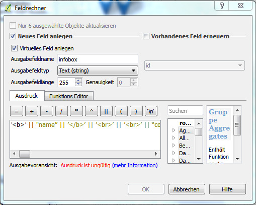
Abbildung 4: Feldrechner mit der Expression, die das zusätzliche virtuelle Feld „infobox“ mit HTML-Text füllt.

HTML Image Map Creator

Nun sind wir fast bereit, um die Webkarte zu erstellen. Wenn gewünscht, kann in der QGIS-Map View noch eine Untermenge der Objekte selektiert werden, die später als Marker auf der Karte erscheinen sollen.

In jedem Falle muss in QGIS ein passender Layer als aktiver Layer selektiert sein, bevor der HTML Image Map Creator gewählt wird (hier der Miet-Pedalos-Layer). Gültige Layer sind Vector-Layer vom Typ Punkt (Point oder Multi-Point) oder Fläche (Polygon oder Multi-Polygon).

Sind alle diese Vorarbeiten gemacht, kann das Plugin in QGIS über das Menü Web => HTML Image Map Creator => Create map… geöffnet werden.  

Der HTML Image Map Creator besteht aus einem einzigen Konfigurationsdialog (vgl. Abbildung 5). Im oberen Bereich des Dialogs findet sich eine kurze Beschreibung. Darunter sind die verschiedenen Informations- und Konfigurationsfelder, auf die im nächsten Abschnitt genauer eingegangen wird.

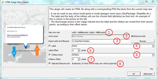
Abbildung 5: Konfigurationsdialog vom HTML Image Map Creator im QGIS. 

Der Konfigurationsdialog

Das erste Feld im Dialog ist ein Informationsfeld, das die Grösse des Map View, also des sichtbaren Kartenausschnitts in QGIS anzeigt. Diese Pixel-Werte müssen gegebenenfalls an das Layout der Publikation angepasst werden - zum Beispiel 800 Pixel breit und 600 Pixel hoch - indem man das Plugin verlässt, die Map View anpasst und dann das Plugin wieder öffnet.

Das zweite Feld „Active layer“ ist ebenfalls ein Informationsfeld. Dieses zeigt den Namen des aktiven Layers an. Ausserdem wird rechts neben dem Textfeld die Anzahl Objekte im Layer angezeigt. Dabei werden auch Objekte ausserhalb der Map View mitgezählt.

Das dritte Feld ist für die Namensgebung und die Wahl des Speicherortes der zu generierenden Dateien zuständig. Mit dem Knopf „Browse“ kann der Benutzer entscheiden, wo er seine Dateien abspeichern möchte und wie er sie benennen will. Alle Dateien werden beim gleichen Pfad abgespeichert. Wir wählen als Namen “Miet-Pedalos”.

Das vierte Feld ist eine Checkbox und eine Dropdown-Liste. Die Checkbox bestimmt, ob das Objekt auf der Karte als Label beschriftet wird. Der Benutzer muss dazu ein Feld des Layers wählen. Die Beschriftung wird mittig unter dem Marker platziert.

Das fünfte Feld dient der Label-Platzierung. Positive Offset-Werte führen zu einer Verschiebung nach unten, negative nach oben.

Das sechste Feld muss - wie bei "Label” - mittels Checkbox aktiviert werden. Es aktiviert die Infoboxen im Export. Wieder muss man ein Feld des Layers wählen. Wir empfehlen ein virtuelles Feld im Feldrechner von QGIS anzulegen (vgl. oben). Falls nicht schon getan, muss man das Plugin verlassen und kann es wieder öffnen, wenn das virtuelle Feld bereit ist.

Das siebte Feld dient der Infobox-Platzierung. Positive Offset-Werte führen zu einer Verschiebung nach unten, negative nach oben.

Das achte und letzte Zeile zeigt eine Checkbox “Selected features only” und eine kleine Statistik. Die Checkbox bestimmt, ob nur die ausgewählten Objekte exportiert werden. Die kleine Statistik zeigt wie viele Objekte im Layer ausgewählt wurden und wie viele dieser Objekte innerhalb der Map View sind.

Nachdem der Benutzer alle Felder ausgefüllt hat, kann ganz unten im Dialog der OK-Knopf gedrückt werden, der den Export startet.

Falls der Export erfolgreich war, sind nun folgende drei Dateien erzeugt worden:

Miet-Pedalos.html: beinhaltet den HTML5-Code (HTML, CSS, Javascript) inkl. den Image Map-Daten der POIs.

Miet-Pedalos.png: ist eine Raster-Grafik-Datei; sie enthält die Basiskarte und wird von HTML-Datei aufgerufen.

Miet-Pedalos.pgw.: ist eine Hilfsdatei (”Worldfile”), die v.a. von Geo-Informationssystemen gelesen wird, um die Karte weiterzuverarbeiten. Sie kann bei reinen Publikationen weggelassen werden.

Diese Dateien (v.a. die .png-Datei und der entsprechende Code-Abschnitt in der .html-Datei) können nun in einen eigenen Blog-Post eingebettet werden und gegebenenfalls angepasst werden. Es kann auch nur die Grafik-Datei Miet-Pedalo.png verwendet werden.

In jedem Falle ist es dem Autor überlassen, mit allen Mitteln, die QGIS zur Verfügung stellt, eine informative Karte zu entwerfen. Nun steht einer informativen Sommergeschichte nichts mehr im Wege!

P.S. Das HTML Image Map Creator QGIS Plugin ist Open Source und wurde in Python geschrieben. Feedback und weitere Software-Kontributoren sind herzlich willkommen!

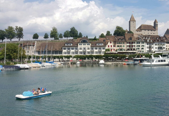
Abbildung 6: Abkühlung für den heissen Sommer: Miet-Pedalo im Zürichsee.

[geometalab]

Building Addresses in OpenStreetMap

Introduction 

Adding a building address to OpenStreetMap may sound too easy for you as to write a blog post specifically about it. However, it can be more complex as you may think. In this blog post - which continues our series of blogposts about “Targeted editing in OpenStreetMap” - we will explain the different ways to correctly enter a building address.

Essential building properties

Before we explain the details of the different methods, we will clarify which properties are essential for the correct mapping of buildings:

building = * marks that the selected area is a building outline and not for example a meadow or a lake. The tag value marks the building type: building = residential for example marks a residential building, building = yes just marks that it is a building, without specifying which type of building it is. You can find all building types on the OSM-Wiki.

addr:street name of the street that belongs to the address.

special case: If the house number is not tied to the street but rather to the name of a “place” (be it a place, a hamlet or something else), then you need to add that name with addr:place and not addr:street.

addr:housenumber (house number of the building).

Different methods

In OpenStreetMap there is more than one method to correctly map a building address. In the following section, we will explain the four approaches known to us in detail.

1. An address for a whole building

On the building outline you directly set the street with addr:street and the related house number with addr:housenumber.

Figure 1: Properties of a building with address on outline way.

2. An address per entrance

If a building has more than one address (for example a multi-family house), then the address can be attached to a building entrance. To define an entrance, you set a node on the outline way. On said node, you set entrance to yes. Now you can set the address to that node by using addr:street for the street name and addr:housenumber for the house number.

Figure 2: Properties of two segments of a multi-family house with different addresses, which have been set to the entrances.

3. Addresses for places within buildings

If a building contains multiple addresses (for example a shopping mall), then you can set the individual addresses using nodes. That for, you place a node within the area with a separate address (generally within a bigger building outline). Now you can set a street name with addr:street and a house number with addr:housenumber.

4. House numbers evenly (linear) distributed on a line

OpenStreetMap supports the so-called house number interpolation, which is suitable for streets, where the house numbers are not distributed by counting trough or even randomly but are distributed by distance (for example road running meters). To use the house number interpolation you need to set nodes on the first and on the last house of the houses you want to interpolate and define them as addresses with a street (addr:street) and the related house number (addr:housenumber). After that, you need to connect these two address nodes with a line. Now you can select the line and set the property addr:interpolation. From there on you can choose if the “to-be-distributed-house-numbers” should be even or odd.

Figure 3: House number interpolation of a row of houses with nodes on the first and the last house.

Conclusion

As you can see, the correct handling of building addresses in OpenStreetMap can be quite challenging in the beginning. However, you just need a push in the right direction, like this post, and everyone can master even this integral part of OpenStreetMap. As long as you keep doing it, mapping is going to get easier and the results will increase in quality. Have fun mapping!

[geometalab]

Gebäudeadressen in OpenStreetMap

Einleitung

Eine Gebäudeadresse in OpenStreetMap hinzuzufügen, hört sich wohl viel zu einfach an, als dass man dafür einen Blogpost schreiben müsste. Doch ist die Sache bei genauerem Hinschauen anspruchsvoller als man denkt. In diesem Blogpost, welcher unsere Reihe über "Targeted Editing in OpenStreetMap” fortsetzt, erläutern wir, welche Möglichkeiten es gibt, um eine Gebäudeadresse korrekt einzutragen.

Wichtige Gebäudeeigenschaften

Bevor wir auf die Details der einzelnen Varianten eingehen, stellen wir klar, welche Eigenschaften essentiell für das korrekte Mappen von Gebäuden sind:

building = * kennzeichnet, dass die markierte Fläche einen Gebäudeumriss angibt und nicht z.B. eine Wiese oder einen See. Der Tag-Value teilt den Gebäude-Typ mit: building = residential zeichnet z.B. ein Wohngebäude aus, building = yes sagt nur, dass es sich um ein Gebäude handelt, ohne den Typ zu spezifizieren. Alle Gebäudetypen findet man auf dem OSM-Wiki.

addr:street Name der zur Adresse gehörenden Strasse.

Spezialfall: Bezieht sich die Hausnummer nicht auf eine Strasse, sondern auf den Namen eines „Orts“ - sei es ein Platz, ein Weiler oder etwas Anderes - so ist dieser Name als addr:place anstatt als addr:street einzutragen.

addr:housenumber Hausnummer des Gebäudes.

Verschiedene Vorgehensweisen

In OpenStreetMap gibt es mehr als eine Möglichkeit, um eine Gebäudeadresse korrekt zu mappen. Im folgenden Abschnitt werden die vier uns bekannten Varianten beschrieben:

1. Eine Adresse für ein ganzes Gebäude

Man setzt auf dem Gebäudeumriss direkt die zugehörige Strasse mittels addr:street und mit addr:housnumber die dazugehörige Hausnummer.

Abbildung 1: Eigenschaften eines Gebäudes mit Adresse auf Umriss-Way.

2. Eine Adresse pro Eingang

Hat ein Gebäude mehrere Adressen (z.B. ein Mehrfamilienhaus), so kann die Adresse an einen Eingang angehängt werden. Um einen Eingang zu definieren, benutzt man einen Node auf dem Umriss-Way. Auf besagtem Node kann man dann die Eigenschaft entrance=yes setzen. Danach kann man diesem Node einen Strassennamen mittels addr:street und eine dazugehörige Hausnummer mittels addr:housenumber hinzufügen.

Abbildung 2: Eigenschaften von 2 Segmenten eines Mehrfamilienhauses mit verschiedenen Adressen, die bei den Eingängen gesetzt wurden.

3. Adressen für Orte innerhalb von Gebäuden

Falls ein Gebäude selbst mehrere Adressen beinhaltet (z.B. ein Einkaufszentrum), so kann man die einzelnen Adressen mittels Nodes setzen. Dazu platziert man einen Node innerhalb der Gebäudeumrisses mit eigener Adresse. Nun kann man den einzelnen Nodes wie gewohnt eine Hausnummer (addr:housenumber) und einen Strassennamen (addr:street) geben. 

4. Hausnummern gleichmässig (linear) auf Linie verteilen

Letztlich unterstützt OpenStreetMap auch die sogenannte Hausnummern-Interpolation, die sich für Strassen eignet, bei denen die Gebäude regelmässig aufsteigend nummeriert sind, gerade Nummern auf der einen, ungerade auf der anderen Strassenseite. Dafür setzt man beim ersten und letzten Haus je einen Node und definiert beide als Adresse mit zugehöriger Strasse (addr:street) sowie der jeweiligen Hausnummer (addr:housenumber). Danach zieht man eine Linie, welche diese beiden Punkte verbindet. Nun kann man der Linie die Eigenschaft addr:interpolation verleihen und sogleich angeben, ob die zu verteilenden Hausnummern auf dieser Strassenseite gerade (= even) oder ungerade (= odd) sind.

Abbildung 3: Hausnummer-Interpolation einer Häuserreihe mit Start- und Endpunkt

Schlusswort

Wie man also sehen kann, mag der richtige Umgang mit Gebäudeadressen in OpenStreetMap fürs Erste ein wenig herausfordernd sein. Doch die Realität verlangt, dass auch die Daten entsprechend erfasst werden. Wir hoffen, mit diesem Blogpost das Mappen ein wenig verständlicher gemacht zu haben und wünschen frohes Mappen!

[geometalab]

How Rapperswil turned into 3D with OpenStreetMap

We introduce ourselves

Welcome to a series of blog posts about making a 3D model of the real world using OpenStreetMap and the related activity we call mapping. We, Severin Fritschi and Emil Sivro, interns at the Institute for Software at HSR, will give you an initial insight into your mapping adventure.

Introduction

When we first heard about OpenStreetMap, abbreviated OSM, almost all of it was new to us. In order to be able to enter the vast world of OSM, we were referred to the OSM-Wiki and LearnOSM, and shortly after we received a first "Mapping" assignment. Once we got familiar with using the OSM webpage, our assignment was to map the houses in the old town of Rapperswil or rather to fill out their properties as close to reality as possible, so that extern “3D renderers” like for example F4map or OSM2World can display them correctly. There are multiple usages for that like for example:

Good basis for developing virtual reality games

Manage an otherwise not manageable area like the Central Park (getting an overview)

Planning festivals or other big public events

Resource for analysing shadows

Hereby we are reporting our experience with OSM, hoping that we can motivate some people to try OSM themselves, as well as pass on our knowledge to tomorrow's mappers.

Precise procedure: simple building

As a mapping example, we will take a simple building located in Rapperswil. When mapping a simple building many things are very easy since you can get a good picture of the building area or roof shape. Most of the time you can even see them clearly. The selection of the roof shape is simplified by the OSM-Wiki.

In the following picture you can see all of the predefined roof possibilities.

Figure 1: Predefined simple roof shapes (source: OSM-Wiki).

Should the roof, which you want to map, have a more complex roof shape, which under circumstances can be a combination of the predefined roofs, you should consider asking an experienced mapper for help, since it is a complicated process. You set the roof shape via the property roof:shape. If nothing else is set the roof will always run along the longer edge (roof:orientation = along). If this should not be the case and the roof of the building runs along the shorter edge, you can set that via roof:orientation = across.

Fine-tuning

When mapping precisely, a trip to the real outside world is inevitable. With help of a “color picker app” you can determine the building colour and roof colour pretty close to actual reality and add them to OSM as properties. In our specific example we used the app “ColorHelper” from the app store. When using such an app, you need to be careful since the display of colours on pictures may vary because of daytime and

Weather. The building height and the roof height are set via building:levels (unit in floors) and roof:height (unit in meters). The roof shape and the building shape are set via the properties building:colour and roof:colour and the associated colours. Also you can set, with which material the building has been built. Note: If you set colour and material as building or roof properties, different renderers will have different results. For example F4Map will always display the set colour. The properties have not been combined but rather material was overwritten by colour. Nevertheless it is good to set both properties since the interpretation varies from renderer to renderer.

In the follosing figure 2 are a few sample images to illustrate the mapping process.

Figure 2: From left to right: Building from F4Map, building from OSM, properties table from OSM.

Conclusion

As it is shown from the pictures, the mapping and tagging of simple buildings is quite simple and easy to learn for everyone. It does not require any topological or geometric knowledge to mark a small house in OSM, nor do you need extensive geographic knowledge to define the roof color and shape, type of building, etc., since you can look up everything on the OSM-Wiki. The effect, on the other hand, is enormous. So it was possible in an adventurous way to present a part of Rapperswil in 3D in a relatively short time and to learn a lot about our environment, which we will continue to do in the future. For this reason, we can recommend the mapping with OSM to everyone, because even the smallest contribution improves the most comprehensive open world map, which we call OpenStreetMap.

[geometalab]

Wie Rapperswil mit OpenStreetMap zu 3D wurde

Wir stellen uns vor

Willkommen zu einer Reihe von Blogposts über OpenStreetMap, die damit verbundene Tätigkeit des Mappens und wie man dadurch ein 3D-Modell der realen Welt erhält. Wir, das sind Severin Fritschi und Emil Sivro, Praktikanten am Institut für Software an der HSR, werden euch hierbei auf eurem Mapping-Abenteuer einen ersten Einblick gewähren.

Einleitung

Als wir zuerst von OpenStreetMap, abgekürzt OSM, hörten, war vieles für uns noch Neuland. Um zuerst einmal in die Welt von OSM eintauchen zu können, wurden wir auf das OSM-Wiki und LearnOSM verwiesen und erhielten sogleich einen ersten „Mapping“-Auftrag. Einmal auf der OSM-Karte zurecht gefunden, ging es darum, die Häuser in der Altstadt in Rapperswil zu mappen, sprich deren Eigenschaften so realitätsnah wie möglich in OSM festzuhalten, sodass diese von externen „3D-Renderern“, wie beispielsweise „F4map“ oder „OSM2World“, visualisiert werden können.

Dies kann unter anderem folgenden Nutzen haben:

Datengrundlage für die Entwicklung von Virtual-Reality-Spielen

Überblick über Gebiet verschaffen, wie z.B. den Central Park

Festivals oder andere Veranstaltungen planen

Räumliche Analysen z.B. von Gebäideschatten

Hierbei berichten wir nun von unseren bisherigen Erfahrungen mit OSM um unser Wissen an die Mapper von morgen weiterzugeben und in der Hoffnung, den einen oder anderen motivieren können, sich selbst an OSM zu versuchen.

Vorgehen: Einfaches Gebäude

Als Beispiel zum Mappen nehmen wir ein simples Gebäude aus Rapperswil. Beim Mappen von einfachen Gebäuden fällt vieles leicht, da man sich mit den Luftbildern meist ein gutes Bild von der Gebäudefläche und der Dachform machen kann oder sie oft sogar deutlich erkennt. Die Auswahl des Daches wird einem durch den Editor und das OSM-Wiki vereinfacht.

Wir verwenden hier eine Vorlage namens “Simple 3D_buildings”. In folgender Abbildung 1 sieht man alle vordefinierten Möglichkeiten einer Dachform.

Abbildung 1: Vordefinierte simple Dachformen aus dem OSM-Wiki.

Man legt die Dachform mit der Eigenschaft roof:shape fest. Es wird angenommen, dass die Dachform entlang der langen Kante verläuft (roof:orientation = along). Ist dies nicht der Fall und das Dach des Hauses verläuft entlang der kürzeren Kante, kann man das mittels roof:orientation = across festlegen.

Sollte das Gebäude, das man mappen will, eine komplexere Dachform haben als in Abbildung 1 vorgegeben, sollte man sich zuerst hier im OSM-Wiki erkundigen, und dann ggf. einen erfahrenen Mapper anfragen.

Feinschliff

Beim genauen Mappen von Gebäuden bleibt der Gang an die Frischluft nicht erspart. Mit Hilfe einem „Color Picker“ kann man Gebäude- und Dach-Farben bestimmen und in OSM als Eigenschaft hinzufügen. In unserem Beispiel wurde der „ColorHelper“ aus dem App Store verwendet, es gibt auch Webtools (z.B. colorpicker.com). Dabei ist zu beachten, dass man beim Benutzen der App nicht immer die genaue Farbe des Gebäudes kriegt, da diese auf Fotos zu verschiedenen Tageszeiten und Witterungen verschieden angezeigt werden.

Die Dach- und Gebäudehöhe wird mittels building:levels (Einheit in Stockwerken ohne das Dach) und roof:height (Einheit in Metern) festgelegt. Die Dach- und Gebäudefarbe wird mit den Eigenschaften building:colour und roof:colour und die dazugehörigen Farben festgelegt. Man kann auch angeben, aus welchem Material das Gebäude und das Dach bestehen mittels building:material und roof:material. Jedoch ist dabei zu beachten, dass wenn colour und material an einem Gebäude oder dessen Dach festgelegt sind, die verschiedenen Renderer unterschiedlich konfiguriert sind. F4map z.B. zeigt dann nur noch die angegebene colour an, d.h. dass das material von colour überschrieben wird. Trotzdem ist es gut, wenn möglich immer beide Eigenschaften einzutragen.

Es folgen noch ein paar Beispielbilder zur Veranschaulichung des Mapping-Prozesses (Abbildung 2):

Abbildung 2: Von links nach rechts: Gebäude aus F4map, Gebäude aus OpenStreetMap, Eigenschaftentabelle aus dem OpenStreetMap-Wiki.

Schlusswort

Wie aus den Bildern hervorgeht, ist das Mapping und Tagging von einfachen Gebäuden ziemlich simpel und somit für jedermann leicht erlernbar. Es bedarf keiner besonderen geographischen Kenntnisse, um ein kleines Häuschen in OSM zu markieren, noch braucht man ein Fachwissen zur Festlegung von Dachfarbe und -form, Art des Gebäudes etc., da man alles im OSM-Wiki nachschlagen kann. Die Wirkung hingegen ist enorm.

So war es uns auf abenteuerliche Art und Weise möglich, in relativ kurzer Zeit einen Teil von Rapperswil in 3D aufzuarbeiten und dabei noch so manches über unsere Umgebung zu lernen. Aus diesem Grund können wir das Mappen mit OSM allen empfehlen, denn auch schon der kleinste Beitrag verbessert die umfangreichste frei zugängliche Weltkarte, die wir OpenStreetMap nennen.

[geometalab]

OSMNames: Free Street/Place Names Database from OpenStreetMap

Modern websites are using more and more maps, and there is a growing need to search for place names in order to locate oneself geographically. This search for a coordinate given a place name is enabled by a geocoding or gazetter service - and this service needs data.

OSMNames is a new open source project which offers a geonames database. Thanks to being based on OpenStreetMap it covers the whole planet and has a clear open license (ODbL). The dataset currently consists of street names, villages, towns and city names together with their areal extent (bounding box), the country they are in and their “importance”. This dataset can be naturally extended in the near future with topographic names (like lakes or mountains; see Toponymy) and even POIs. This enables coarse-grained (”street-level”) geocoding.

Figure: Homepage of OSMNames.org - The street/place names database with easy delivery and installation, clear licensing and clear code!

Postal addresses (house numbers) and zip codes are not included because they are of separate nature: They are typically of point geometry type and their fuzzy search and display formatting is kind of black magic. In addition, they often are related to private organizations and sometimes have unclear licensing. Thus postal addresses probably are a separate kind of data set suitable for fine-grained geocoding (as described in Wikipedia; see also e.g. openaddresses.io).

This data is delivered in Tab Separated Value (TSV) format. It’s content is quite similar to parts of Nominatim. For example, the importance of place names is calculated by using Wikipedia data and actually Nominatim tools are used for accomplishing this.

The workflow to produce this worldwide data has been dockerized so that it can be easily deployed on any system. The simplicity of the installation and the clear arrangement of code plus the fast processing time make this open source project unique.

The OSMNames database has been successfully integrated in a coarse-grained geocoder webservice by Klokan Technologies (see this

blog post

) which uses Sphinx for parsing and geocoding.

We invite all to join us over at GitHub to set up a worldwide, openly licensed database!

Give OSMNames a spin at http://osmnames.org !