#Central Limit Theorem

[emmy-noethers-rings]

feel free to reblog. “sample size” and all that

[micandrea]

sooooooo exhausted. weekend was awful :( and i don't understand math

[wordacrosstime]

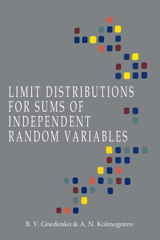
Limit Distributions for Sums of Independent Random Variables

[Limit Distributions for Sums of Independent Random Variables, by BV Gnedenko (Author), AN Kolmogorov (Author), KL Chung (Translator). Paperback (Reprint of the 1954 Edition) - 5 Aug 2021. Publisher - Martino Fine Books (5 Aug 2021). Language - English. Paperback - 276 pages. ISBN-10 - 1684225795. ISBN-13 - 978-1684225798. Dimensions - 15.6 x 1.57 x 23.39 cm. (details thanks to Amazon)]

[Author full names: Boris Vladimirovich Gnedenko (Russian: Бори́с Влади́мирович Гнеде́нко; 1 January 1912 – 27 December 1995); Andrey Nikolaevich Kolmogorov (Russian: Андре́й Никола́евич Колмого́ров, IPA: [ɐnˈdrʲej nʲɪkɐˈlajɪvʲɪtɕ kəlmɐˈɡorəf], 25 April 1903 – 20 October 1987) (details thanks to Wikipedia)]

***

A number of years ago I set about a course of self-improvement. For me that meant reading as much as possible from works written by world-class thinkers. This list of august minds was often, though not solely, driven by Nobel Prize winners and other winners of similar or equivalent awards in other areas (mathematics, for example, where the Fields Medal and Abel Prize are the highest honors). However, I am a statistician among other things, and so I have also kept a keen eye out for important works by the giants of that field.

I am not well-acquainted with Boris Gnedenko, though his name has certainly come up from time to time over the years that I’ve both studied and practiced statistics. The name that has come up repeatedly in reverential tones is Andrey Kolmogorov, who is one of a handful of mathematicians who are credited with giving the theoretical underpinnings of statistics a solid and rigorous mathematical foundation.

The volume under review here is one of Kolmogorov’s most important publications. In it, he and Gnedenko elicit the basis and application of results like the Central Limit Theorem (CLT) and the Law of Large Numbers (LLN). These are two of the most important results in all of statistics and probability theory and the slightly more general theory of stochastic (random) processes.

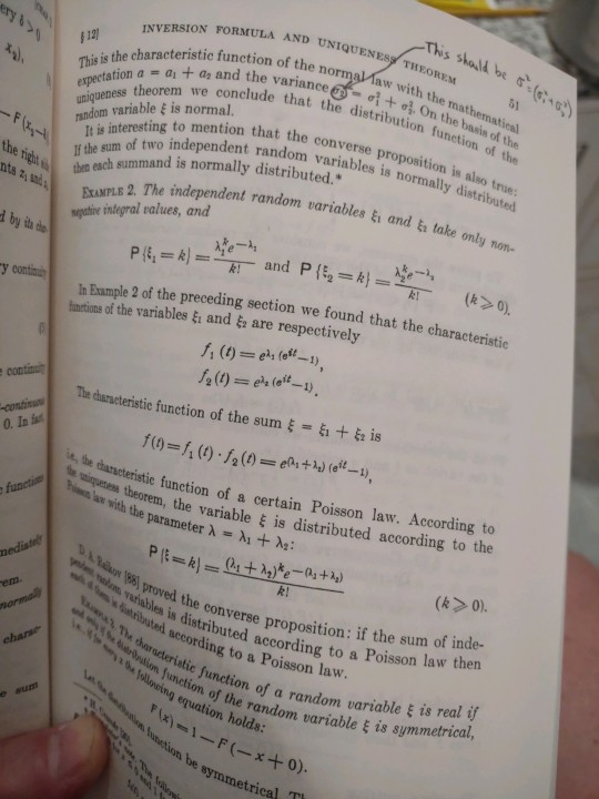
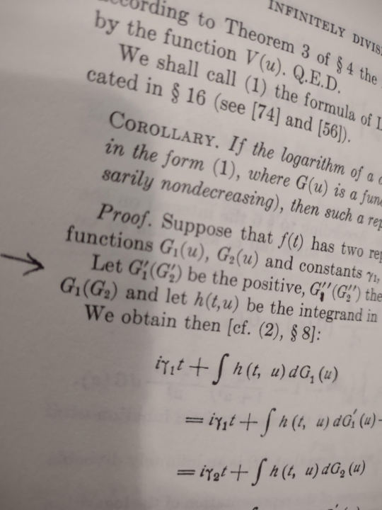
I should mention that this volume was originally published in the Soviet Union in 1949 in Russian. The edition I read here was translated into English in 1954 by KL Chung, and the actual ISBN citation is this particular reprint; there are others from different time periods, and of course if one is a true purist, then one should definitely read the original Russian text. However, according to the preface, all of the formulas and other special figures in the text are actually photostats from the original monograph.

I really enjoyed this book. The writing style of Gnedenko and Kolmogorov is delightfully lofty and at times quite flowery, but their explanations of proofs and motivations for results are really first-rate. I wasn’t sure what to expect, given the high intellectual bar these gentlemen set, but I was very pleasantly surprised. Professor Chung, the translator, added quite a few helpful comments and clarifications where appropriate, but overall he seems to have let the book flow as it was originally set down. One of the Appendices was written by another legendary statistician, JL Doob, providing a bit of bridge material related to some measure-theoretic issues that arise in Chapter 1.

My only complaint (a very small one to be sure) is that there were a number of typos that remained intact despite the extensive editorial review this monograph has surely had over the past 70+ years. I wouldn’t exactly call it a super-power, but I personally seem to have a knack for finding typos and grammatical errors in even very technical material. I’ve taken photos of two of the ones I found early in the text as examples here (see below). For some reason my eye was instinctively drawn to these and others. I would thus advise the reader to pause if something seems slightly amiss – it very well might be. I’m happy to say that these errata were few and far between, and in no case do I recall them rendering the explanations or results indecipherable.

Who would enjoy this tome? Anyone who is interested in the theoretical basis for many of the classic results in modern non-Bayesian statistics. The foreword by the translator advises that a solid background in calculus is a must, and mathematical maturity a definite plus. Beyond that, the book itself is remarkably self-contained. This is likely due to the political environment in which it was written. Post-World War II was a difficult time for Soviet intellectuals since they were generally denied access to journals and results outside their own country.

Here are the two examples of typos that I detected early in the book – I think they speak for themselves, but you can be the judge:

[Image credits numbered from top: (1 & 2) two pages from the book photographed by reviewer- with thanks to © publishers and estates of authors. (3 & 4) book cover front and back - with thanks to © publishers (5) Boris Vladimirovich Gnedenko - with thanks, no details of © copyright holder / photographer known (6) Andrey Nikolaevich Kolmogorov - with thanks, no details of © copyright holder / photographer known]

Kevin Gillette

Words Across Time

12 January 2024

wordsacrosstime

[sandu-zidian]

Pride and Prejudice read through I got to the Darcy proposal… holy shit I was not expecting it to happen then and the revelations after 😭😭😭

[buthappysoverrated]

do you think math student liebgott works or

[streetlight-haver]

i use my CLT for means til i normally distribute

[monado-stew]

something downright sexual about the way that you can force pretty much any average value to act like a normal distribution if you've got a large enough sample size

[monocotyledons]

every once in a while i rediscover 3blue1brown and go through a binge watching period of watching the videos i missed and rewatching his older videos that are my faves like wow i love his stuff so much

[darkmaga-retard]

I'll show you the easiest way to do that in this article. However, it doesn't appear that any of the New Zealand lawmakers or health authorities are interested in what the data shows.

Steve Kirsch

Sep 14, 2024

Executive summary

Recently, I took another look at the New Zealand data leaked by Barry Young.

It turns out it is trivial to show that the 1 year mortality from the time of the shot is batch dependent, varying by a factor of 2 or more. That’s a huge problem for the mean mortality rates to have such a huge variation.

The other important realization (that I’m apparently the first person to point out) is that for a given age range and vaccination date, if you do a histogram of the mortality rates of the batches, if the vaccines are safe, these will form a normal distribution because of the central limit theorem. That simply doesn’t happen. So that’s another huge red flag that the vaccines are not safe.

The code and the data

The code for the New Zealand batch analysis was trivial to write. It can be found in my NewZealand Github.

Batches vary by over 2X in mortality rate, even if they are given in the same month to the same age range of people

You can’t have a 2X variation in the 1-year mortality rate for a given vaccination date and 5 year age range. That suggests that the vaccine is not safe. We can do a Fisher exact test to prove our point.

Let’s take the 80-84 year old line because there are lots of deaths there so it’s easier to show the differences between the batches are statistically significant (which should never happen if the vaccines are all safe).

Statistics for batch 34 vs. batch 38 for ages 80 to 84 given Jan 1, 2022 to Feb 28, 2022. The Fisher matrix is (5381 2859 139 194 8573).

One-sided p-value 7.956587575710554e-18 Max likelihood estimate of the Odds ratio= 2.6265352736010104 95% Confidence Interval(low=2.091, high=3.305)

So we’re done. You can try values higher than 34 and you’ll see this wasn’t cherry picked. The 2X variation is easy to find and is statistically significant when we have enough data in the batches.

[emmy-noethers-rings]

Broke: any random variable is Gaussian ↯

Woke: any sun of random variables is Gaussian

Bespoke: any sun of n > 60 random variables is Gaussian

[yourbestamericangirlmp3]

horse plinko central limit theorem

[taumoeba]

Yall need to start romanticizing learning statistics because I cant scroll past another tumblr poll post (which i cant even see on tumblr mobile) with wrong terminology.... "Reblog bc we need a larger sample size for more accurate results" how about randomization to control for selection bias 😂😂😭 central limit theorem is not going to save you

[nostalgebraist]

Another way to look at the Kelly criterion is to think about betting on a variable number of independent things at once.

If you make a single bet repeatedly, and you use the Kelly criterion, then over time, your log(wealth) is a sum of IID random variables.

So the Law of Large Numbers and Central Limit Theorem hold...

asymptotically, as time passes

for log(wealth)

Now imagine that instead, you diversify your wealth across many identical and independent bets. (And you use Kelly to decide how to bet on each one, given the fraction of wealth assigned to it.)

Here, the limit theorems hold...

asymptotically, as the number of simultaneous bets grows

for wealth

which is better in both respects. You control the number of bets, so you can just set "n" to a large number immediately rather than having to wait. And the convergence is faster and tighter in term of real money, because the thing that converges doesn't get magnified by an exp() at the end.

This is regular diversification, which is very familiar. And then, making sequential independent bets turns out to be kind of like "diversifying across time," because they're independent. But it's not as nice as what happens in regular diversification.

In fact, the familiar knee-jerk intuition "never go all-in, bet less than everything!" comes from this distinction, rather than from any result about how to bet on a single random variable if forced to do so.

In the real world, you're not stuck in an eternal casino with exactly one machine. If you keep some money held back from your bet, it doesn't just sit there unused. Money you hold back from a bet can be used for things, including other independent bets.

(The Kelly criterion holds money back so it can be used on future rounds of the same bet, which are a special case of "other independent bets.")

Of course, if you have linear utility (i.e. no risk aversion), you should still go all-in on whichever bet has highest expected return individually. If this were really true, your life would be so simple that most of finance would be irrelevant to it (and vice versa). You'd just put 100% in whichever asset you thought was best at any given time.

[naveenkrishna002]

Unveiling Market Insights: Exploring the Sampling Distribution, Standard Deviation, and Standard Error of NIFTY50 Volumes in Stock Analysis

Introduction:

In the dynamic realm of stock analysis, exploring the sampling distribution, standard deviation, and standard error of NIFTY50 volumes is significant. Providing useful tools for investors, these statistical insights go beyond abstraction. When there is market volatility, standard deviation directs risk evaluation. Forecasting accuracy is improved by the sample distribution, which functions similarly to a navigational aid. Reliability of estimates is guaranteed by standard error. These are not only stock-specific insights; they also impact portfolio construction and enable quick adjustments to market developments. A data-driven strategy powered by these statistical measurements enables investors to operate confidently and resiliently in the financial world, where choices are what determine success.           

NIFTY-50 is the tracker of Indian Economy, the index is frequently evaluated and re-equalizing to make sure it correctly affects the shifting aspects of the economic landscape in India. Extensively pursued index, this portrays an important role in accomplishing, investment approach ways and market analyses.

Methodology

The data was collected from Kaggle, with the (dimension of 2400+ rows and 8 rows, which are: date, open, close, high, low, volume, stock split, dividend. After retrieving data from the data source, we cleaned the null values and unnecessary columns from the set using Python Programming. We removed all the 0 values from the dataset and dropped all the columns which are less correlated.

After completing all the pre-processing techniques, we imported our cleaned values into RStudio for further analysis of our dataset.

Findings:

Our aim lies in finding how the samples are truly representing the volume. So, for acquiring our aim, we first took a set of samples of sizes 100 and 200 respectively. Then we performed some calculations separately on both of the samples for finding the mean, standard deviation, sampling distribution and standard error. At last we compared both of the samples and found that the mean and the standard deviation of the second sample which is having the size of 200 is more closely related to the volume.

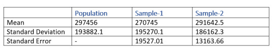
From the above table, the mean of the sample-2 which has a size of 200 entity is 291642.5 and the mean of the sample-1 is 270745. From this result, it is clear that sample-2 is better representative of the volume as compared to sample-1

            Similarly, when we take a look at the standard error, sample-2 is lesser as compared to sample-1. Which means that the sample-2 is more likely to be closer to the volume.

Population Distribution.

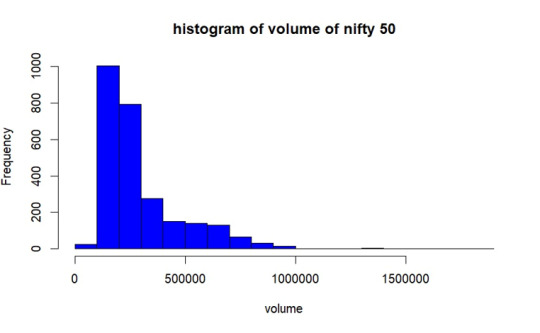
As per the graph, In most of the days from the year 2017 to 2023 December volume of trading of NIFTY50 was between 1lakh- 2.8lakhs.

Sample Selection

We are taking 2 sample set having 100 and 200 of size respectively without replacement. Then we obtained mean, standard deviation and standard error of both of the samples.

Sampling Distribution of Sample- 1

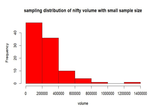
From the above graph, the samples are mostly between 0 to 2 lakhs of volume. Also, the samples are less distributed throughout the population. The mean is 270745, standard deviation is 195270.5 and the standard error of sampling is 19527.01.

Sampling Distribution of Sample- 2

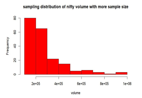
From the above graph, the samples are mostly between 0 to 2 lakhs of volume. Also, the samples are more distributed than the sample-1 throughout the volume. The mean is 291642.5, standard deviation is 186162.3 and the standard error of sampling is 13163.66.

Replication of Sample- 1

Here, we are duplicating the mean of every sample combination while taking into account every conceivable sample set from our volume. This suggests that the sample size is growing in this instance since the sample means follow the normal distribution according to the central limit theorem.

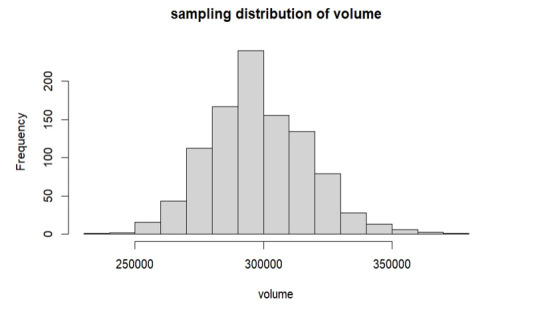
As per the above graph, it is clear that means of sample sets which we have replicated follows the normal distribution, from the graph the mean is around 3 lakhs which is approximately equals to our true volume mean 297456 which we have already calculated.

Conclusion

In the observed trading volume range of 2 lakhs to 3 lakhs, increasing the sample size led to a decrease in standard error. The sample mean converges to the true volume mean as sample size increases, according to this trend. Interestingly, the resulting sample distribution closely resembles the population when the sample mean is duplicated. The mean produced by this replication process is significantly more similar to the population mean, confirming the central limit theorem's validity in describing the real features of the trade volume.