#Delete blank columns in excel vba

[feelvewor]

Delete blank columns in excel vba

Delete blank columns in excel vba how to#

Delete blank columns in excel vba code#

Delete blank columns in excel vba free#

Covering all of the cases exceeds the scope of this VBA tutorial. The criteria you use to identify those columns varies from case to case. In order to delete columns using VBA, the first thing you need to do is identify which columns to delete. For a thorough explanation of VBA loops, you can refer to the detailed tutorial I prepared here. I provide a very basic explanation of these constructs in the relevant sections below. The following sections introduce several VBA constructs that may help you in each of these steps.įurther to the above, some of the sample macros below rely on the following 2 VBA structures: Delete the complete columns you've selected.Identify the columns you want to delete.If you want to create a macro to delete columns with VBA, you'll generally proceed in the following 3 steps: Let's start then by taking a look at some… Excel VBA Constructs To Delete Columns Books Referenced In This Excel VBA Tutorial.Macro Example #8: Delete Columns Based On Header Contents.Macro Example #7: Delete Columns Based On Cell Value.Macro Example #6: Delete Columns Based On Header (String).Macro Example #4: Delete Columns With Blank Cells.Excel Macro Examples #1 To #3: Delete Specific Column(s).Relevant VBA Structures To Delete Columns.Step #3: Delete Cells With The Range.Delete Method.The following table of contents lists the main topics I cover within this VBA tutorial:

Delete blank columns in excel vba free#

You can get immediate free access to this example workbook by subscribing to the Power Spreadsheets Newsletter. This Excel VBA Delete Column Tutorial is accompanied by an Excel workbook containing the data and macros I use in the examples below.

Delete blank columns in excel vba how to#

For example, if your objective is to delete empty columns (like example #5 below) or columns with blank cells (code example #4 below), the examples within my blog post on how to delete blank rows or rows with empty cells can provide further guidance. Therefore, I try to cover a wide variety of circumstances in the examples below.ĭepending on the particular case you're working on, other tutorials within Power Spreadsheets may also help you craft the precise macro you need to delete columns. I'm aware that, depending on the situation, you may use different criteria to determine the columns that Visual Basic for Applications deletes.

Delete blank columns in excel vba code#

Each of these macro code examples is accompanied by a detailed step-by-step explanation.

Show you 8 different sample macros that you can easily adjust and start using immediately to delete columns.

Explain some of the most common VBA constructs that you can use to delete columns.

In this particular Excel tutorial, I focus on explaining several ways in which you can automate the deletion of columns using VBA macros. At the same time, if you set up your macros properly, they can reduce the risk of mistakes during the process. At the same time, it's important to ensure the accuracy of the data you're using for your analysis.Įxcel VBA macros can help you automate some data-cleanup activities. You're probably aware that the process of cleaning up data can be annoying and time consuming.

[wbspeedsite]

Visual basic for applications examples

Here we find the Last used Row in the Sheet #19 – Find the Last Used Column in the Sheet #18 – Find the Last Used Row in the Sheet 'Note: RmDir delete only a empty folder On Error GoTo 0 End SubĬhange the folder path, which is marked in red as per your folder deletion. RmDir "C:UsersAdmin_2.Dell-PcDesktopDelete Folder" 'Firstly it will delete all the files in the folder 'Then below code will delete the entire folder if it is empty 'You can use this to delete entire folder On Error Resume Next Error Resume Next VBA On Error Resume Statement is an error-handling aspect used for ignoring the code line because of which the error occurred and continuing with the next line right after the code line with the error. Kill "C:UsersAdmin_2.Dell-PcDesktopDelete Folder*.*"Ĭhange the folder path, which is marked in red as per your folder deletion. '' On Error Resume Next Error Resume Next VBA On Error Resume Statement is an error-handling aspect used for ignoring the code line because of which the error occurred and continuing with the next line right after the code line with the error. 'You can use this to delete all the files in the folder Test The above code hides all the sheets except the sheet named “Main Sheet.” You can change the worksheet name as per your wish. If Ws.Name "Main Sheet" Then Ws.Visible = xlSheetVeryHidden It will highlight all the blank cells with green color. Result: #13 – Highlight All the Blank Cellsĭ(xlCellTypeBlanks).Interior.Color = vbGreenįirst, select the data range and run the code. #12 – Highlight All the Commented CellsĬode: Sub HighlightCellsWithCommentsInActiveWorksheet()Ī(xlCellTypeComments).Interior.ColorIndex = 4 It will convert all the text values to lower case characters in excel Lower Case Characters In Excel There are six methods to change lowercase in excel - Using the lower function to change case in excel, Using the VBA command button, VBA shortcut key, Using Flash Fill, Enter text in lower case only, Using Microsoft word. #11 – Change All To Lower Case Charactersįirst, select the data and run the code. It will convert all the text values to upper case characters. #10 – Change All To Upper Case Charactersįirst, select the data and run the code. It will highlight the cells which have spelling mistakes. If Not Application.CheckSpelling(Word:=MySelection.Text) Thenįirst, select the data and run the VBA code VBA Code VBA code refers to a set of instructions written by the user in the Visual Basic Applications programming language on a Visual Basic Editor (VBE) to perform a specific task. #9 – Highlight Spelling Mistakeįor Each MySelection In ActiveSheet.UsedRange #8 – Insert Blank Row After Every Other RowĬode: Sub Insert_Row_After_Every_Other_Row()ĭim rng As Range Dim CountRow As Integer Dim i As Integer Set rng = Selectionįor this first, you need to select the range where you would like to insert alternative blank rows. This will delete all the blank worksheets from the workbook we are working on. If WorksheetFunction.CountA(ws.UsedRange) = 0 ThenĪpplication.ScreenUpdating = True End Sub #7 – Delete All Blank Worksheets From the WorkbookĪpplication.ScreenUpdating = False For Each ws In ActiveWorkbook.Worksheets Just specify the number in the input box and click on Ok, it will insert those many sheets immediately. This will ask you to enter the number of worksheets you would like to insert. If ShtCount = False Then Exit Sub Else For i = 1 To ShtCount ShtCount = Application.InputBox("How Many Sheets you would like to insert?", #6 – Insert Worksheets as Much as You want This will insert serial numbers from 10 to 1 from the top. This will insert serial numbers from 1 to 20 from the bottom.

This will insert serial numbers from 1 to 10 from the top. Let’s see each of these examples in detail. Delete All Blank Worksheets From the Workbook.Source: VBA Examples () List of Top 19 Examples You are free to use this image on your website, templates etc, Please provide us with an attribution link How to Provide Attribution? Article Link to be Hyperlinked Ok, if you struggled with VBA and still a beginner in this article, we will give some of the useful examples of VBA Macro code in Excel. I know oftentimes you might have thought of some of the limitations excel has but with VBA coding, you can eliminate all of those. Right from small tasks to big tasks, we can automate by using the VBA coding language. Macros are your best friend when it comes to increase your productivity or save some time at your workplace.

[milascl]

Removing hyperlinks in excel 2016

REMOVING HYPERLINKS IN EXCEL 2016 CODE

You have been able to remove all hyperlinks with a small bit of Excel VBA code. This instruction was already entered into the module for us when started the type the name of the Macro.

REMOVING HYPERLINKS IN EXCEL 2016 CODE

Once of all of the looping of worksheets has been completed then the code finally ends. If the used range in each of the worksheets contains hyperlinks they are deleted. The next link of code looks at the used range in each of the worksheets. Looping is usually used when we need to perform the same activity over and over again in the workbook. The line of code will loop through each of the worksheets in the current workbook. I have created the variable as below to store the worksheet names. This simply creates a memory container for the values. Now all that is needed is the rest of the code in between these two lines of code.įirst, I need to declare a variable in this macro. Why Is My Personal Macro Workbook Not Loading Automatically?Ĭreate A Shortcut To Your Personal Excel Macro Workbook Write The Code To Remove Hyperlinks.Īs you type the name of the Macro and hit return, Excel will automatically insert End Sub. To remove more than one hyperlink, select a range containing multiple hyperlinks (such as a range. In Excel 2010/2013, click File > Options and in Excel 2007, click Office button > Excel Options to open the Excel Options dialog. A: Excel 2010 provides a new option called Remove Hyperlinks (pluralwith an s) that enables you to remove multiple hyperlinks (prior editions of Excel provide only the Remove Hyperlink option, which removes only one hyperlink at a time). The build-in Autocorrect Options in Excel can help you to disable the automatic hyperlinks when you enter the web address. If you want more details on creating and updating your personal macro workbook then I recommend my blog posts below.Ĭreating and Updating Your Personal Macro Workbook Prevent automatic hyperlinks with Autocorrect Options in Excel. So, I will make sure to save this in my Personal Macro Workbook. This is a really useful macro that I want to reuse over and over again. Clear cells, tables, hyperlinks, styles, formulas, shapes or charts of Excel XLS, XLSX, XLSM, XLSB, CSV, TXT, Tab Delimited, TSV and OpenDocument ODS files, remove blank rows / columns, remove. By default, this macro workbook is named Personal.xlsb. There are several ways to paste special in Excel, including right-clicking on the target cell and selecting. Now you can select all those by holding the shift key convert those formulas to values by using paste special Using Paste Special Paste special in Excel allows you to paste partial aspects of the data copied. When you select this option then Excel creates (if it is not already created) this workbook and saves the macro in that location. The results of all the external links will be shown in the same dialogue box. In this instance, I may want to reuse the code so I will store it in my Personal Macro Workbook. If you store it in the current workbook then use is restricted to that workbook. If you save the code in your Personal Macro workbook it will be available in any Excel workbooks. What Is The Difference In The Locations?. To store your code either in your Personal Macro Workbook or.Before you begin to write any code you need to decide where to store the code.

[manvewor]

Easy way to delete empty rows in excel

Now there are 2 ways to delete blank rows. Then under Home> Cells> Delete> Delete sheet rows. The advise given is on the Home tab> Editing> Find & Select> Go to Special> Blanks. The Safe Definition Of Devops Includes Which Three Concepts? 10. You need to place the cursor in the first blank row of the (28)….Remove All Blank Rows from Bottom/a Range in Excel Office 365!! When you bring data from another source into an Excel worksheet, the data often includes rows that you’ll want to delete. How to Delete Blank or Unneeded Rows, Method 1 All of your rows beneath with automatically be (26)… 9. The empty row will be deleted, and the rows beneath will move up to fill the empty space. If you have several blank rows one 3.Select “Delete”. You’ll see the entire empty row get selected when you right-click. If you only have a row or two that you need to delete, you can quickly do it with your mouse.2.Right-click on the row number that you want to delete. Right-click the selected row and delete the row ġ4 steps1.Find the row that you want to remove. Click on the row number on the left to select Select the entire dataset (A1:C13 in this (24)….Go to each blank row and delete it manually (too tedious and time-consuming). Delete Blank Rows in Excel (with and without VBA) In this blog, we’ll teach you how get rid of (23)… 8. Sometimes in an Excel sheet, blank rows make it harder to focus and may cause some errors. You do not need to select the entire data (22)… Steps to Remove Blank Cells or Rows from a Range in Excel Select the column or row that contains the blank cells. If you have an Excel spreadsheet with blank rows, you can delete them all at once rather than having to do them one at time. How To Delete Blank Rows In Excel – The Florida Bar Click OK and then all the blank rows/cells (20)… 7. Go to the tab “DATA”-“Data Tool”-“Delete Duplicates”. To remove the same rows in Excel, select the entire table. How to Remove a Bigger Number of Blank Rows from a Large Table If you want to remove the blank rows in a table, go to ‘Home’ tab, group ‘Editing’ and click on (18)… On the Home tab, click to open the drop-down menu beneath ” (17)… To remove blank rows in the table, hold “Ctrl” and click one cell in each row you want to remove. How to Delete Blank Rows in Excel | Techwalla Hold your Ctrl/Control key as you select each row. If you spot several blank rows, you can remove them all at once. If there are few Empty Rows to delete in an Excel worksheet, you can manually delete them by right-clicking on the row and selecting the Delete option in (14)…Ĭlick Kutools > Delete > Delete Blank Rows, then in the sub drop-down list, choose one operation as you need. How to Hide or Delete Empty Rows in Excel – Techbout Manually Deleting Blank Rows in Excel The easiest way to remove blank rows is to select the blank rows manually and delete them. If you now click “Entire row”, Excel removes the entire (12)… In the “Home” tab, you will find the option “Delete cells…” under the option “Delete”. The simple way to remove an individual blank row, or even a few next to each other, is to select them, which you can do by clicking their number (11)… To select multiple rows, press Ctrl and (9)…Īt this point, to delete the empty rows, go to the Home ribbon and click the drop-down of the Delete button in the Cells group. Select a row by clicking on the row number on the left side of the screen.How to Remove Blank Rows in Excel the Easy Way Go to the Ablebits Tools tab > Transform group.How to remove empty rows in 4 easy steps Click its heading or select a cell in the row and press Shift + spacebar. How to Delete Blank Rows in Excel (5 Fast Ways to Remove …Įasy Ways to Remove Blank or Empty Rows in Excel In the Go to Special dialogue box, choose Blanks and hit OK. In the resulting Go To dialog box, click Special.(4)…Ī quick way to delete blank rows in Excel Alternatively, select and right-click on the rows which are completely blank. Go to the Home tab and click Delete > Delete Sheet Rows. How to Remove Blank Rows in Excel | GoSkills How To Turn On Cellular Data On Apple Watch? 2.

[strangehoot]

New Post has been published on Strange Hoot - How To’s, Reviews, Comparisons, Top 10s, & Tech Guide

New Post has been published on https://strangehoot.com/how-to-delete-multiple-rows-in-excel-sheet-at-once/

How To Delete Multiple Rows in Excel Sheet at Once

Delete multiple rows in Excel is a task that is done while performing data cleanup. The data cleanup process may be required when we get a dataset from the team we are working with or the vendor with whom we have corporate relations or we ourselves want to perform some predictive analysis in Excel. 

Why there is a need of deleting rows in Excel 

You need to remove a certain segment of data that is not important or there are endless blank cells that you need to delete to evaluate the data or cleaning up the datasheet and making it ready to structure the data. 

When you bring data from another source to the Excel worksheet, the imported data contains unwanted blank rows / columns in between and you want to erase them. 

You may want to delete multiple rows in Excel which are irrelevant data. When dealing with large data sets, you will need to delete multiple rows quickly to save time. As working with large data in the Excel sheet requires a lot of time performing the steps. It is necessary to know shortcuts and perform the steps faster to finish the task quickly.

Excel Features 

Microsoft Excel has so many useful features that project managers and analysts maintain the projects on MS Excel. Let us see some interesting features of Excel.

Add Header and Footer:

MS Excel enables you to keep the header and footer in the spreadsheet and when you take the print, you will see header and footer printed on the paper. Usually, company logo and taglines are part of headers and page number and company website URL is part of footer.

Find the order of text and replace it:

MS Excel helps us to locate the appropriate data (text, numbers, alphanumeric) in the workbook and also substitute the current data with a new one. For example, you are searching the text with “Adam”, you will see the cell containing the word and you can use the arrow key to go to the next result of the same word and so on. While formatting the data, you can use the replace feature to replace the found word one by one or all at once.

Filtration of data

Filtering is a fast and simple way to locate and run a subset of data within a range. Only rows that follow the requirements you define for a column are shown in the filtered set. MS Excel offers two filtering range commands: 

AutoFilter, which includes a filter by choice, for simple criteria;

Advanced Filter – to filter with more nuanced criteria.

Post filtering the data, it becomes easier to clean up the data using the “delete multiple rows” action with the options given in Excel.

Sorting of data

Data sorting is the method of organising data in a logical order. MS Excel helps you to sort data in ascending or descending order. You can also define the order of sorting the data. 

Formulae built-in:

Microsoft Excel includes several predefined, or built-in, formulas that are known as functions. 

Functions may be used to render basic or complex calculations. The most widely used function is the SUM function, which is used to add numbers to a set of cells. All complex mathematical formulas are available as built-in is used for quick calculation for larger datasets. Manually working on formulas is time consuming. Excel helps us to do the calculations quicker and easily.

Auditing Formula

Using formula auditing, we can graphically view or trace the relationship between cells and formulas with blue arrows. Precedents (cells that provide data to a specific cell) or dependents (cells that depend on the value in a specific cell) may be tracked.

Build Pivot Table and Charts (Pivot Table Report):

Creating a Pivot table for the data given in Excel is simpler. Arranging the dataset manually again is a question of correctness. There might be errors doing manual tasks. Excel gives functionality to generate Pivot within a fraction of a minute.

MS Excel helps us to construct various visual charts, such as bar graphs, pie-charts, line graphs, etc. This helps us interpret and compare data very quickly. Analysis related tasks are done easily generating charts from the given data in Excel. 

Security of Excel sheet / workbook using Password Protection

It helps users to protect their workbooks from unauthorised access to their details by using a password.

Add-ins / Macros

Excel offers a variety of add-ins to use certain tasks and calculations. One of them is Analysis ToolPack. For doing calculations of mathematical formulas and running regressions, this add-in is very useful. Running Macros using VBA editor in Excel works as a programming application. You can perform some repeated actions in your dataset using Macros. It is just awesome.

Insert and Delete Columns / Rows [step-by step guide]

There are 16384 total columns available in the Excel Worksheet. When you insert a new column, the total number of columns available in the Excel worksheet will not change. If the last columns (equivalent to the number of columns inserted) in the Excel worksheet are empty, the columns are deleted from the worksheet to accommodate the newly inserted Columns.

Let us see different ways to insert columns in Excel.

Method 1: Using Right-click menu

Open your worksheet with data.

Pick the column where you want to insert a new blank column by clicking on the column letter.

Right-click the column letter of the column immediately to the right of where you intend to insert the new column.

Click Insert from the right-click menu. 

A new column is now added to the left of the column.

Method 2: Using Excel Ribbon

Alternatively, to get the same result is by running the command, Insert Sheet Columns from Excel Ribbon > Insert menu button as shown.

Click Insert Sheet Columns.

Method 3: Using DOSE Add-in

Click DOSE. A toolbar with multiple options will be shown.

From Insert, click the option highlighted with red border.

A new blank column is placed at the position of the selected column. All columns from the position of the selected column are moved to the right to accommodate the newly added column as seen in the image below.

Blank column(s) are inserted in between.

To delete columns, perform the following steps:

Method 1: Using shortcut

Select the column that you want to remove.

Press Ctrl and then, press – . The column will be removed.

Method 2: Using right-click menu

Select columns.

To select more than one column at a time, hold down CTRL and click each applicable letter.

Right-click and select the column(s) you want to delete. In this case, choose the Delete columns B – C option.

To insert rows, perform the following steps.

Method 1: Using right-click

Pick a cell in the row that you want to remove.

Right-click and pick Insert from the pop-up menu.

You will see a new row inserted.

Method 3: Using the row selection

Click on the number associated with the appropriate row to highlight all cells in the row. 

Right-click the highlighted row.

To select more than one row at a time, hold down CTRL and click each applicable number.

To delete rows, perform the following steps. 

Method 1: Using right-click menu

Pick a cell in the row that you want to remove.

Right-click and pick Delete from the pop-up menu.

When the Delete window appears. You have the next option to delete a row or a column. Select row. The selected row will be removed.

Method 2: Using shortcut

Pick the row that you want to remove.

Press CTRL and then press –. The column will be removed.

Delete Multiple Rows in Excel at Once [step-by step guide]

To delete multiple rows at once, perform the following steps.

Method 1: Using shortcut

Open a Microsoft Excel sheet containing a dataset.

Filter the data to get the subset. 

Once filtered, you can select the unwanted rows.

Press CTRL + – to remove the selected rows.

Method 2: Using right-click

Open a Microsoft Excel sheet containing a dataset.

Filter the data to get the subset. 

Once filtered, you can select the unwanted rows.

Right-click and select Delete.

Method 3: Using Go To Special

Open a Microsoft Excel sheet containing a dataset.

On the icon toolbar, click Find & Select.

A menu appears with the list of options. Choose Go To Special.

From the dialog box, choose Blanks and OK.

Blank cells are selected choosing the above option. 

Choose Delete.

From the list of options that appear, choose Delete Sheet Rows.

All blanks with rows are deleted. The sheet will be cleaned up as shown below.

MS Excel is irreplaceable

Excel has strong capabilities to do analysis and execute regression models on the server. It also has a network sharing facility that allows the team to work on the same datasheet. It is a perfect tool for storing data that changes from time to time.

Google sheets, Mac OS Numbers are the spreadsheets with limited features and cannot beat MS Excel. There are scenarios where people use Windows OS only for MS Excel as other operating systems do not give its features in totality.

Knowing how to delete multiple rows in Excel at once is a simple and quick trick on your sleeve.

Read: How to Create a Waterfall Chart in Microsoft Excel?

[enterinit]

Office Insider for Windows Version 2006 release notes

Office Insider for Windows Version 2006 release notes.

Build 12920.20000 (May 29, 2020)

Outlook 

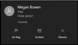
Quick Action buttons now appear in pop-up notifications   You’ll start seeing Quick Action buttons in your pop-up notifications when running Outlook on Windows 10. Now you’ll be able to flag, delete, or complete other actions from the notification. To configure the actions, right click in the Outlook message list and choose Set Quick Actions.  

PowerPoint

Faster playback comes to Microsoft Stream videos  Microsoft Stream lets people in your organization upload, view, and share videos securely. You can share recordings of classes, meetings, presentations, training sessions, or other videos that your team needs. We previously enabled Stream as one of the supported online video sources in PowerPoint. Over the last few months, we've made significant performance improvements to the video playback experience. Now you’ll experience faster playback of Stream videos in your PowerPoint presentations.   Learn more.  Notable fixes: We fixed an issue where slides were not centered after zooming using the mouse wheel.

Word 

Notable fixes: We fixed an issue where copy and pasting text to a comment pane would not be displayed.We fixed an issue where comment hint bubbles appeared blurry at 100% zoom.We fixed an issue where files with long path names (greater than 32K) would not open and an appropriate error message was not being displayed.We fixed an issue where enabling policy Word 2007 and later Binary Documents and Templates would cause some co-authoring cases to fail.

Excel 

Notable fixes: We fixed an issue where Excel would occasionally shut down when engaging OneDrive.We fixed an issue where clicking a bookmarked hyperlink within the same workbook would cause the workbook to be hidden.We fixed an issue where some copy and pasted chart links used mapped drive addresses rather than universal addresses.We fixed an issue where Excel could become unresponsive after using Ctrl+Shift+Arrow keys to scroll when the Excel window was shared through Teams.

Build 12914.20000 (May 22, 2020)

Excel, Word, and PowerPoint  Pin your folders makes saving Office files easier  We received feedback that users want more control over the folders available when a new file is saved. We're excited to bring a new capability to you: pin your folders in the Save dialog. This new capability will make saving your Word, Excel, and PowerPoint files easier.  Learn more.  

Excel  Notable fixes: We fixed an issue where the error message “This workbook is currently referenced by another and cannot be closed” would appear because add-ins were being loaded in alphabetical order rather than in a user specified order.We fixed an issue where memory was being corrupted when managing fonts between Excel and some third-party assistive technology applications.We fixed an issue where Excel would crash when add-ins ask for Host Items on worksheets that contain shapes with noSelect locks. Word  Notable fixes: We fixed an issue where hyperlinks in comments weren’t working.We fixed an issue where pasting HTML into WordMail for Calendar wasn’t working.We fixed an issue where replying to a comment in a co-authored session could sometimes cause Word to freeze.We fixed an issue where zooming in and out from the presentation area resulted in a gap between the zoomed selection marquee and the mouse pointer.We fixed an issue where Word would crash when add-ins ask for Host Items on documents that contain shapes with noSelect locks. PowerPoint   Notable fixes: We fixed an issue where zooming in and out from the presentation area resulted in a gap between the zoomed selection marquee and the mouse pointer. Outlook  Notable fixes: We fixed an issue where the Folder.BeforeItemMove event didn't fire correctly when a user moved items between folders.We fixed an issue where users saw calendar items that spanned the midnight threshold as All day events.We fixed an issue where Outlook crashed when two add-ins added a button to the same group in the ribbon.We fixed an issue where users were unable to share a calendar with a guest user.

Project 

Notable fixes: We fixed an issue where Project would crash after clicking on Options.

Build 12905.20000 (May 15, 2020)

PowerPoint  Use your Surface Earbuds to control your PowerPoint presentations  If you forget your clicker or don’t want to use, your Surface earbuds have you covered. You can swipe forward and backward on the left earbud to navigate your presentation when it is in Slide Show mode. You can play or pause videos embedded in your presentation by double tapping.   How it works: Once paired, you'll need to enable the feature in PowerPoint.   Start a presentation by pressing F5 or selecting Slide Show > From Beginning.In Slide Show, right click on the slide and under Surface Earbuds Settings choose Use Gestures to Control Presentation. This setting will be remembered for all future presentations. Learn more.

Notable fixes: We fixed an issue where keyboard shortcuts and spell check wouldn’t function as expected when using an English Switzerland (QWERTZ) keyboard. Excel   Import and refresh data from PDF documents   We’re excited to announce that the #9 request on the Data Import related asks on Excel UserVoice is now available. You can now import and analyze data from PDF documents. To enable this feature, select the Data tab > Get Data > From Files > From PDF.   Notable fixes: We fixed an issue that caused printer names to be duplicated in the list of available printers.We fixed an issue that resulted in improved performance time for users when they deleted merged columns. Outlook  Find just what you need Narrow your search with options like folder, sender, date, attachment info, and more. Word  Notable fixes: We fixed an issue where files with custom xml values opened extremely slowly.We fixed an issue where inserting or updating an Index in a document containing more than a hundred entries would result in the application crashing.We fixed an issue where adding a new comment on a blank document wouldn't do anything. Office Suite   Notable fixes: We fixed an issue in Visual Basic for Applications in Microsoft Office where certain VBA projects that contain references to code libraries with double-byte characters in the library name or library path would be viewed by the Office application as corrupt on load. Read the full article

[siva3155]

300+ TOP MS EXCEL Interview Questions and Answers

MS EXCEL Interview Questions for freshers and experienced :-

1. What is Microsoft Excel Microsoft Excel is said to be a spreadsheet application or an electronic worksheet that is helpful for storing, analyzing data, manipulating data, and organizing reports. 2. Provide the different types of data formats available in Excel Accounting, Date, Percentage, Number, and Text are the different data formats available in Excel. 3. Define Format Painter If you want to copy the format of a cell, text, image etc and apply on another text, the Format painter is used. 4. Define cells in Excel The place where we store the data is called a cell. 5. Why to use comments in Excel? Comments in Excel are used to describe a formula given in a cell and leave notes for the users for any extra/special information. 6. How will you add comments in Excel? To add comments in Excel, perform the below actions: Right-click on the cell Select “Insert” from the toolbar Click “Comment”. Comment box appears. You can enter the required information here. 7. List out the charts available in MS Excel Pie, Bar, Scatter, Line are some of the available charts in MS Excel, which is useful to provide graphical representation of a report/analysis. 8. What is Ribbon in Excel A specific area that runs at the top of the application, comprised of toolbar and menu items is called a Ribbon. There are various tabs available in ribbon containing a set of commands to use in the application. 9. What is the shortcut key to hide the ribbon in Excel? Ctrl+F1 is the shortcut key to hide the ribbon in Excel 10. How will you protect a sheet in Excel? To protect the worksheet in Excel, navigate to Menu bar -> Review -> Protect sheet -> Password. Provide a password to protect the worksheet and avoid copying the data.

MS EXCEL Interview Questions 11. What is the function used to get the total of columns and rows in Excel? To get the total of columns and rows in Excel, use the function ‘SUM’. 12. How many report formats are available in Excel? Report, Compact and Tabular are the formats available in Excel. 13. What is the use of ‘IF’ function in Excel? To verify whether the conditions are true or false, the function ‘IF’ is used in Excel. 14. Give the advantage of Look Up function in Excel To return a value for array, you can use the function Look Up 15. What is the shortcut key to delete the blank columns? To delete the blank columns in Excel, press Ctrl+-. 16. How many rows and columns are present in Microsoft Excel 2013? There are 1048576 rows and 16384 columns in Microsoft Excel 2013. 17. Provide the syntax for VLookUp The syntax for VLookUp is given below: VLOOKUP(lookup_value,table_array,col_index_num,) 18. How the errors are highlighted in Excel? The different errors displayed in Excel are #REF!, #DIV/0!, #NUM, #N/A, #NAME, and #VALUE!. 19. While evaluating formulas in Excel, what is the operations order used? PEMDAS is the acronym given for the order of operations in Excel. P – Parenthesis/ Brackets E – Exponentiation (^) M – Multiplication D – Division A – Addition S – Subtraction 20. Provide the major functions performed in Excel The major functions performed in Excel are SUMIF, INDEX/MATCH, VLOOKUP, IFERROR and COUNTIF. 21. In excel, what is the function used to get the length of a string? Use the function ‘LEN’ to find the text string length. 22. Describe volatile functions When there is a modification performed in the worksheet, make use of volatile function to recalculate the formula repeatedly. 23. Provide the list of volatile formulas TODAY(), NOW(), and RAND(. are the highly volatile formulas. INDIRECT(), OFFSET(), INFO(), and CELL(. are the other volatile formulas. 24. Provide the shortcut for find and replace Ctrl+F is the shortcut key to open the find tab and Ctrl+H is the shortcut to open find and replace tab. 25. How will you open the spellcheck dialog box using a shortcut key? To open a spell-check dialog box, the shortcut key is F7. 26. To perform auto-sum on the rows and columns, what is the shortcut? ‘ALT=’ is the shortcut to perform auto-sum on the rows and columns. 27. How will you open a new Excel workbook using a shortcut key? Ctrl+N is the shortcut to open a new Excel workbook. 28. Can you give us the different sections in a Pivot Table? Filter Area, Columns Area, Values Area, and Rows Area are the sections available in Pivot Table. 29. What is Slicer in Excel The 2010 version Excel has the feature called Slicer in Pivot Table. With the help of Slicer in Pivot table, users can filter the data while selecting one or more options in slicer box. 30. Who designed the Bullet Chart? Stephen Few is a dashboard expert who designed Bullet Charts and this chart has been extensively acknowledged as one of the topmost graphical representation to show the performance report. 31. What are the different types of data filter available in Excel? Date filter, Text Filter and Number Filter are the different types of data filter available in Excel. 32. What are the popular methods to transpose a data set in Excel? Using Transpose function and Paste Special Dialog Box are the two (2. methods to transpose a data set in Excel. 33. Is it possible to remove duplicates in Excel from a data set? There is an in-built feature in Excel to remove duplicates from a data set. Steps to remove duplicates is given below: Select Data -> Select ‘Data’ tab -> Click ‘Remove Duplicates’. 34. Provide the two macro languages available in MS Excel Visual Basic Applications (VBA. and XLM are the two (2. macro languages available in MS Excel. 35. Mention the event used to check the status of a Pivot Table modification Use the event ‘PivotTableUpdate’ to check the status of a Pivot Table modification in a worksheet. 36. What is the syntax of SUBSTITUTE function in Excel? Syntax of SUBSTITUTE function in Excel: ‘SUBSTITUTE(text, oldText, newText, )’ 37. What is the syntax of REPLACE function in Excel? Syntax of REPLACE function in Excel: REPLACE(oldText, startNumber, NumberCharacters, newText) 38. What are the keys used to move to the previous worksheet in Excel? The keys Ctrl + PgUp is used to move to the previous worksheet in Excel 39. What are the keys used to move to the next worksheet in Excel? The keys Ctrl + PgDown is used to move to the previous worksheet in Excel 40. Which filter is used to analyse the list that is employed with database function? Advanced Criteria Filter is used to analyse the list employed with database function. 41. What is the shortcut key to minimize the workbook? The keys ‘Ctrl+F9’ is the shortcut key to minimize the workbook. 42. How will you cancel an entry using the shortcut key? ‘Esc’ key is used to cancel the entry in Excel. 43. Will we be able to change the font and color of the multiple sheet tabs? Yes, we can easily change the font and color of the sheet tabs in Excel. 44. What are the key elements to give a best dashboard? The key elements such as Minimum distractions, visual presentation of information, easy to communicate, and provide useful data to the business stands out to be the best dashboard. 45. What are the new enhancements available in Excel latest version? Slicers, Tables, IFERROR, Powerpivot, and Sparklines are the new enhancements available in Excel latest version. 46. Is it possible to close all the open excel files at a time? Yes, it is possible to close all the open excel files at a time. 47. In Excel, what is Name Manager? We give a name for a cell or a Range which is called Name Manager. Using the Name manager, Table gets managed. 48. Which symbol is used to lock or fix the reference? The symbol ‘$’ is used to lock or fix the reference. 49. What is the advantage of Freeze panes in Excel? If you want to lock a specific column or row, Freeze panes can be used. 50. Do you think we have unique address for each cell? Yes, we have a uniue address for each cell based on the value of the row and column. MS EXCEL Questions and Answers Pdf Download Read the full article

[seotipsandtricks-me]

Here’s a list of some of the less well known Excel formulas and macros that regularly come in handy for keyword marketers. That could be SEOs, PPCs or anyone who works with large spreadsheets containing keywords and associated data like search volume, CPC & categories. Think of it as an excel cheat sheet designed for keyword marketers, but useful for anyone wanting to grow their Excel bag of tricks. Enjoy! FORMULAS Get domain from URL Get subdomain from URL Remove first x characters from cell Remove last x characters from a cell Group keyword phrases automatically based on words they contain Word count Find out if a value exists in a range of other values Get true or false if a word or string is in a cell Remove first word from cell (all before & including 1st space) Replace the first word in a cell with another word Super trim – more reliable trimming of spaces from cells Perform text-to-columns using a formula Extract the final folder path from a URL Extract the first folder path from a URL Remove all text after the xth instance of a specific character Create an alphabetical list of column letters for use in other formulas Count instances of a character in a cell Count the number of times a specific word appears in a cell Return true if there are no numbers in a cell Get the current column letter for use in other formulas Put your keywords into numbered batches for pulling seasonal search volume data Word order flipper Find the maximum numerical value in a row range, and return the column header Find position of nth occurrence of character in a cell Get all characters after the last instance of a string Get all characters after the first instance of a string Get URL path from URL in Google Analytics format Get the next x characters after a string VBA Convert all non-clickable URLs in your spreadsheet to clickable hyperlinks Conditional formatting by row value Remove duplicates individually by column Merge adjacent cells in a range based on identical value Remove all instances of any text between and including 2 characters Highlight mis-spelled words Lock all slicers in position Split delimited values in a cell into multiple rows with key column retained Make multiple copies of a worksheet at once Add a specific number of new rows based on cell value Column stacker Superfast find and replace for huge datasets Paste all cells as values in a worksheet in the active range Format all cells to any format without having to select them Formula activation – insert equals at the beginning for a range of cells Consolidate all worksheets from multiple workbooks into one workbook Fast deletion of named columns Find and replace based on a table Unhide all sheets in a workbook Change pivot table data source for all pivot tables on a worksheet Convert all ‘numbers stored as text’ to general     Get domain from URL: =LEFT(A2,FIND("/",A2,9)) This works by bringing back everything to the left of the first trailing slash found after the initial 2 in ‘http..://’, which in a URL is the slash occurring after the TLD.   Get subdomain from URL: =IF(SUBSTITUTE(SUBSTITUTE(SUBSTITUTE(SUBSTITUTE(LEFT(A2,FIND(".",A2)),"http://",""),".",""),"https://",""),"domain","")="","none",SUBSTITUTE(SUBSTITUTE(SUBSTITUTE(SUBSTITUTE(LEFT(A2,FIND(".",A2)),"http://",""),".",""),"https://",""),"domain","")) When you just need the subdomains in a big list from a bunch of differently formatted URLs. This formula works regardless of the presence of the protocol. What it lacks in elegance, it more than makes up for in usefulness.   Remove first X characters from cell: =RIGHT(A1,LEN(A1)-X) If there’s something consistent that you want to remove from the front of data in your cells, such as an html tag like

, you can use this to remove it by specifying its length in characters in this formula, so X would be 7 in this case.   Remove last X characters from a cell: =LEFT(B2,LEN(B2)-X) You might use this to remove the trailing slash from a list of URLs, for example, with X as 1.   Group keyword phrases automatically based on words they contain: =IFERROR(LOOKUP(2^15,SEARCH($C$2:$C$200,A2),$D$2:$D$200),"/") This little chap deserves a blog post all its own. Here’s what it does: Example: Bulk categorisation of keywords by colour and hair type groups. Using the formula to group your keywords: $C$2:$C$200 is your string-to-search-for range (the list of all the possible words you want to check for in the keyword). $D$2:$D$200 is your Label to return when string found, put it in the next column along lined up (this can just be the word you’re checking for if you want – same as above) A2 is the cell containing the keyword string which you are searching to see if it contains any of the listed strings so you can label it as such “/” is what gets returned when none of the strings are matched Using the formula   Word count: =IF(LEN(TRIM(A2))=0,0,LEN(TRIM(A2))-LEN(SUBSTITUTE(A2," ",""))+1) See how many words are in your keyword to identify if it’s long tail and get a measure of potential intent.   Find out if a value exists in a range of other values: =ISNUMBER(MATCH(A2,B:B,0)) This is my favourite, so often we just need to know if URLs in list A are contained within list B. No need to count vlookup columns or iferror. It gives TRUE or FALSE.   Get TRUE or FALSE if a word or string is in a cell: =ISNUMBER(SEARCH("text-to-find",A2)) If you fancy a break from using the ‘contains’ filter, this can be a way to get things done faster and in a more versatile way.   Remove first word from cell (all before & including 1st space): =RIGHT(A2,LEN(A2)-FIND(" ",A2)) To remove the last word instead, just use LEFT instead of RIGHT.     Replace the first word in a cell with another word: =REPLACE(A2,1,LEN(LEFT(A2,FIND(" ",A2)))-1,"X") “X” is the word you want to replace the incumbent first word with, or this can be a cell reference.     Super trim – more reliable trimming of spaces from cells: =TRIM(SUBSTITUTE(A2,CHAR(160),CHAR(32))) Sometimes using =TRIM() fails because of an unconventional space character from something you’ve pasted into Excel. This gets them all.   Perform text-to-columns using a formula: =TRIM(MID(SUBSTITUTE($A2," ",REPT(" ",LEN($A2))),((COLUMNS($A2:A2)-1)*LEN($A2))+1,LEN($A2))) This is handy for template building. It provides a way of doing text-to-columns automatically with formulas, using a delimiter you specify. In the example, space ” ” is used as the delimiter.     Extract the final folder path from a URL: =IF(AND(LEN(A2)-LEN(SUBSTITUTE(A2,"/",""))=3,RIGHT(A2,1)="/"),"",IF(RIGHT(A2,1)="/",RIGHT(LEFT(A2,LEN(A2)-1),LEN(LEFT(A2,LEN(A2)-1))-FIND("@",SUBSTITUTE(LEFT(A2,LEN(A2)-1),"/","@",LEN(LEFT(A2,LEN(A2)-1))-LEN(SUBSTITUTE(LEFT(A2,LEN(A2)-1),"/",""))),1)),RIGHT(A2,LEN(A2)-FIND("@",SUBSTITUTE(A2,"/","@",LEN(A2)-LEN(SUBSTITUTE(A2,"/",""))),1)))) Good for when you need to get just the last portion of a URL, that pertains to the specific page:   Extract the first folder path from a URL: =IF(LEN(A2)-LEN(SUBSTITUTE(A2,"/",""))>3,LEFT(RIGHT(A2,LEN(A2)-FIND("/",A2,9)),FIND("/",RIGHT(A2,LEN(A2)-FIND("/",A2,9)))-1),RIGHT(A2,LEN(A2)-FIND("/",A2,9))) Good for extracting language folder.   Remove all text after the Xth instance of a specific character: =LEFT(A2,FIND(CHAR(160),SUBSTITUTE(A2,"/",CHAR(160),LEN(A2)-LEN(SUBSTITUTE(A2,"/",""))-0))) Say you want to chop the last folder off a URL, or revert a keyword cluster to a previous hierarchy level. The “/” is the character where the split will occur, change it to whatever you want. The “-0” at the end chops off everything after the last instance. Changing it to -1 would chop off everything after the penultimate instance, and so on.   Create an alphabetical list of column letters for use in other formulas A,B,C…AA,BB etc: =SUBSTITUTE(ADDRESS(1,ROWS(A$1:A1),4),1,"") Unlike with numbers, Excel doesn’t automatically give you the next letter of the alphabet if you drag down after selecting cells with ‘a’ and ‘b’ but you can use this to achieve that effect. It runs through the columns, so it will keep working past Z, giving you AA and AB etc. That’s handy for making indirect references in formulas.   Count instances of a character in a cell: =LEN(A2)-LEN(SUBSTITUTE(A2," ","")) Countif “*”&”x”&”*” doesn’t cut it for this task because it counts cells, not occurrences. The example here is for ” ” space character.   Count the number of times a specific word appears in a cell: =(LEN(A2)-LEN(SUBSTITUTE(A2,B2,"")))/LEN(B2) The formula above works for individual characters, but if you need to count whole words this will work – handy for checking keyword inclusion in landing page copy for SEO. In the example, B2 should contain the word you are counting the instances of within A2.   Return TRUE if there are no numbers in a cell: =COUNT(FIND({0,1,2,3,4,5,6,7,8,9},B28))<1 Change the end to >0 to show TRUE if there are numbers present. Handy for isolating and removing cells of data which can be identified as unwanted by the presence or absence of a number, such as a mix of item names and item product codes when you only want the item names.   Get the current column letter for use in other formulas: =MID(ADDRESS(ROW(),COLUMN()),2,SEARCH("$",ADDRESS(ROW(),COLUMN()),2)-2) If you’re using indirect references and want a fast way to just get the current column letter placed into your formula, use this.   Put your keywords into numbered batches for pulling seasonal search volume data: =IF(A2=43,1,A2+1) To save you having to count out 2,500 keywords each time. This batches them up so you just have to filter for the batch number, ctrl A, ctrl C, ctrl V – 43 is the number of keywords in your list divided by 2500, which is the keyword planner limit. Use the blank row insertion macro to make the batches easily selectable.     Word order flipper: =TRIM(MID(F18,SEARCH(" ",F18)+1,250))&" "&LEFT(F18,SEARCH(" ",F18)-1) Turns ‘dresses white wedding’ into ‘white wedding dresses’. Use it in steps inside itself to further rearrange words in a different order.   Find the maximum numerical value in a row range, and return the column header: =INDEX($A$1:$F$1,MATCH(MAX(A2:F2),A2:F2,0)) So if your column headers are months or categories, this brings back which one contains the highest value for that row. Useful for showing which month has the highest search volume for a keyword.   Find position of nth occurrence of character in a cell: =FIND(CHAR(1),SUBSTITUTE(A1,"c",CHAR(1),3)) Useful as a part of other formulas.   Get all characters after the last instance of a string: =SUBSTITUTE(RIGHT(A2,LEN(A2)-FIND("@",SUBSTITUTE(A2," > ","@",(LEN(A2)-LEN(SUBSTITUTE(A2," > ","")))/LEN(" > ")))),"> ","") Gets ‘category 3’ from ‘category 1 > category 2 > category 3’, splitting on the last ‘>’.   Get all characters after the first instance of a string: =TRIM(MID(A2,SEARCH(" > ",A2)+LEN(" > "),255)) Like the above, but chops off the first category e.g. gets ‘category 2 > category 3’ from ‘category 1 > category 2 > category 3’, splitting on the first ‘>’.   Get URL path from URL in Google Analytics format: ="/"&RIGHT(A2,LEN(A2)-FIND("/",A2,9)) Gets ‘/folder/file’ from ‘http://www.domain.com/folder/file’, I use this to convert URLs to the path format used in Google Analytics exports when I need to vlookup data from the export into another sheet containing full URLs. You could do a find and replace instead, but that doesn’t catch the subdomains and other oddities you may have in your URL list.   Get the next x characters after a string: This one is cool. If your cell contained ‘product ID:0123 london’, you could tell this formula to get ‘0123’ based on the presence of ‘product ID:’ in front of it. It says ‘find this, and bring back the next x characters’.  =IFERROR(LEFT(RIGHT(A2,LEN(A2)-(SEARCH("STRING",A2)+6)),6),"") There are 3 parts you need to change. Replace STRING with your string to search for e.g. ‘product ID:’ Replace ‘+6’ with the length of your string to search for, so for ‘product ID:’ it would be ‘+11’ Replace the next number, ‘6’, with the number of characters you want to capture after the end of the string to search for. So to capture ‘0123’ from ‘product ID:0123’ you’d put ‘4’. =IFERROR(LEFT(RIGHT(A2,LEN(A2)-(SEARCH("product ID:",A2)+11)),4),"") So it’s a bit like regex capture. I used this to get the width and height of images in raw HTML.   EXCEL VBA  MODULES VBA does stuff to your spreadsheets by pressing a button. Usually this is stuff that would take a long time to do (or be hard / impossible to do) using the normal Excel ribbon & formula capabilities. To use these: Save your workbook as .xlsm Reopen it and hit alt + f11 In the menu, insert > module Paste in the code Press the play button There’s no need to understand the code. But be careful to save a backup copy of your workbook before running any of these – they can’t be undone with ctrl + z!     Convert all non-clickable URLs in your spreadsheet to  clickable hyperlinks: So you can visit the URLs easily if you need to e.g. for optimisation of a lot of pages, so you don’t have to mess about double clicking each one to get it ready. Sub HyperAdd() For Each xCell In Selection ActiveSheet.Hyperlinks.Add Anchor:=xCell, Address:=xCell.Formula Next xCell End Sub     Conditional formatting by row value: So the colour intensity is relative to each row only, rather than the entire range. You need to use this to complete the search landscape document seasonality tab. Sub NewCF() Range("B1:P1").Copy For Each r In Selection.Rows r.PasteSpecial (xlPasteFormats) Next r Application.CutCopyMode = False End Sub     Remove duplicates individually by column: If you have a lot of columns, each of which needs duplicates removing individually e.g. if you have a series of category taxonomies to clean – you can’t do this from the menu: Sub removeDups() Dim col As Range For Each col In Range("A:Z").Columns With col .RemoveDuplicates Columns:=1, Header:=xlYes End With Next col End Sub     Merge adjacent cells in a range based on identical value: To save you doing it individually when you need to make a spreadsheet look good: Sub MergeSameCell() 'Updateby20131127 Dim Rng As Range, xCell As Range Dim xRows As Integer xTitleId = "KutoolsforExcel" Set WorkRng = Application.Selection Set WorkRng = Application.InputBox("Range", xTitleId, WorkRng.Address, Type:=8) Application.ScreenUpdating = False Application.DisplayAlerts = False xRows = WorkRng.Rows.Count For Each Rng In WorkRng.Columns For i = 1 To xRows - 1 For j = i + 1 To xRows If Rng.Cells(i, 1).Value <> Rng.Cells(j, 1).Value Then Exit For End If Next WorkRng.Parent.Range(Rng.Cells(i, 1), Rng.Cells(j - 1, 1)).Merge i = j - 1 Next Next Application.DisplayAlerts = True Application.ScreenUpdating = True End Sub     Remove all instances of any text between and including 2 characters from a cell (in this example, the < and >): Especially good for removing HTML tags from screaming frog extractions, kind of a stand in for regex. Public Function DELBRC(ByVal str As String) As String While InStr(str, "<") > 0 And InStr(str, ">") > InStr(str, "<") str = Left(str, InStr(str, "<") - 1) & Mid(str, InStr(str, ">") + 1) Wend DELBRC = Trim(str) End Function     Highlight mis-spelled words: This can help you identify garbled / nonsense keywords from a large set, or just to spellcheck in Excel if you need to. Sub Highlight_Misspelled_Words() For Each cell In ActiveSheet.UsedRange If Not Application.CheckSpelling(Word:=cell.Text) Then cell.Interior.ColorIndex = 3 Next End Sub     Lock all slicers in position: If you send Excel documents to clients with slicers in them, you might worry that they’ll end up moving the slicers around while trying to use them – a poor experience which makes your document feel less professional.  But there’s a way around it – run this code and your slicers will be locked in place across all worksheets, while still operational. This effect persists when the document is re-saved as a normal .xlsx file. Option Explicit Sub DisableAllSlicersMoveAndResize() Dim oSlicerCache As SlicerCache Dim oSlicer As Slicer For Each oSlicerCache In ActiveWorkbook.SlicerCaches For Each oSlicer In oSlicerCache.Slicers oSlicer.DisableMoveResizeUI = True Next oSlicer Next oSlicerCache End Sub     Split delimited values in a cell into multiple rows with key column retained: It’s easy to put a delimited string (Keyword,Volume,CPC…) into columns using text-to-columns but what if you want it split vertically instead, into rows? This can help: Sub SliceNDice() Dim objRegex As Object Dim X Dim Y Dim lngRow As Long Dim lngCnt As Long Dim tempArr() As String Dim strArr Set objRegex = CreateObject("vbscript.regexp") objRegex.Pattern = "^s+(.+?)$" 'Define the range to be analysed X = Range([a1], Cells(Rows.Count, "b").End(xlUp)).Value2 ReDim Y(1 To 2, 1 To 1000) For lngRow = 1 To UBound(X, 1) 'Split each string by "," tempArr = Split(X(lngRow, 2), ",") For Each strArr In tempArr lngCnt = lngCnt + 1 'Add another 1000 records to resorted array every 1000 records If lngCnt Mod 1000 = 0 Then ReDim Preserve Y(1 To 2, 1 To lngCnt + 1000) Y(1, lngCnt) = X(lngRow, 1) Y(2, lngCnt) = objRegex.Replace(strArr, "$1") Next Next lngRow 'Dump the re-ordered range to columns C:D [c1].Resize(lngCnt, 2).Value2 = Application.Transpose(Y) End Sub     Make multiple copies of a worksheet at once: If you are making a reporting template for example, and want to get the sheets for all 12 weeks created in one go: Sub swtbeb4lyfe43() ThisWS = "name-of-existing-worksheet" '# of new sheets s = 6 '# of new sheets For i = 2 To s Worksheets("name-of-existing-worksheet-ending-with-1").Copy After:=Worksheets(Worksheets.Count) ActiveSheet.Name = ThisWS & i Next i End Sub     Add a specific number of new rows based on cell value: Saves repeatedly using insert row, pressing F4 etc: Sub test() On Error Resume Next For r = Cells(Rows.Count, "E").End(xlUp).Row To 2 Step -1 For rw = 2 To Cells(r, "E").Value + 1 Cells(r + 1, "E").EntireRow.Insert Next rw, r End Sub     Column stacker: This one’s great when you have lots of columns of information that you want to be combined all into one master column: Sub ConvertRangeToColumn() 'UpdatebyExtendoffice Dim Range1 As Range, Range2 As Range, Rng As Range Dim rowIndex As Integer xTitleId = "KutoolsforExcel" Set Range1 = Application.Selection Set Range1 = Application.InputBox("Source Ranges:", xTitleId, Range1.Address, Type:=8) Set Range2 = Application.InputBox("Convert to (single cell):", xTitleId, Type:=8) rowIndex = 0 Application.ScreenUpdating = False For Each Rng In Range1.Rows Rng.Copy Range2.Offset(rowIndex, 0).PasteSpecial Paste:=xlPasteAll, Transpose:=True rowIndex = rowIndex + Rng.Columns.Count Next Application.CutCopyMode = False Application.ScreenUpdating = True End Sub     Superfast find and replace for huge datasets: To match partial cell, change to ‘X1Part”. Sub Macro1() Application.EnableEvents = False Application.ScreenUpdating = False Application.Calculation = xlCalculationManual ' fill your range in here Range("S2:AJ252814").Select ' choose what to search for and what to replace with here Selection.Replace What:="0", Replacement:="/", LookAt:=xlWhole, SearchOrder:=xlByRows, MatchCase:=False, SearchFormat:=False, ReplaceFormat:=False Application.EnableEvents = True Application.ScreenUpdating = True Application.Calculation = xlCalculationAutomatic Application.CalculateFull End Sub     Paste all cells as values in a worksheet in the active range: For when your spreadsheet is too slow to do it manually Sub ToVals() With ActiveSheet.UsedRange .Value = .Value End With End Sub     Format all cells to general format or whatever you like, without having to select them: Another good one for when your spreadsheet is too slow. Sub dural() ActiveSheet.Cells.NumberFormat = "General" End Sub     Formula activation – Insert equals at the beginning for a range of cells: If you’re making something complex with a lot of formulas that you don’t want switched on yet, but you want to be able to use other formulas at the same time (i.e. can’t turn off calculations) this can help. It’s also good for just adding things to the start of cells: Sub Insert_Equals() Application.ScreenUpdating = False Dim cell As Range For Each cell In Selection cell.Formula = "=" & cell.Value Next cell Application.ScreenUpdating = True End Sub     Consolidate all worksheets from multiple workbooks in a folder on your computer into a single workbook with all the worksheets added into it: If you have a big collection of workbooks which you want consolidated into one, you can do it in a single step using this macro. Especially good for when the workbooks you need to consolidate are big and slow. Sub CombineFiles() Dim Path As String Dim FileName As String Dim Wkb As Workbook Dim WS As Worksheet Application.EnableEvents = False Application.ScreenUpdating = False Path = "C:scu" 'Change as needed FileName = Dir(Path & "*.xl*", vbNormal) Do Until FileName = "" Set Wkb = Workbooks.Open(FileName:=Path & "" & FileName) For Each WS In Wkb.Worksheets WS.Copy After:=ThisWorkbook.Sheets(ThisWorkbook.Sheets.Count) Next WS Wkb.Close False FileName = Dir() Loop Application.EnableEvents = True Application.ScreenUpdating = True End Sub     Fast deletion of named columns in a spreadsheet which is responding slowly: Sometimes, one does not simply ‘delete a column’. This is for those times. Sub Delete_Surplus_Columns() Dim FindString As String Dim iCol As Long, LastCol As Long, FirstCol As Long Dim CalcMode As Long With Application CalcMode = .Calculation .Calculation = xlCalculationManual .ScreenUpdating = False End With FirstCol = 1 With ActiveSheet .DisplayPageBreaks = False LastCol = .Cells(3, Columns.Count).End(xlToLeft).Column For iCol = LastCol To FirstCol Step -1 If IsError(.Cells(3, iCol).Value) Then 'Do nothing 'This avoids an error if there is a error in the cell ElseIf .Cells(3, iCol).Value = "Value B" Then .Columns(iCol).Delete ElseIf .Cells(3, iCol).Value = "Value C" Then .Columns(iCol).Delete End If Next iCol End With With Application .ScreenUpdating = True .Calculation = CalcMode End With End Sub     Find and replace based on a table in another worksheet: Use X1Part for string match & replace within a cell, or X1 whole for whole cell match & replace: Sub Substitutions() Dim rngData As Range Dim rngLookup As Range Dim Lookup As Range With Sheets("Sheet1") Set rngData = .Range("A1", .Range("A" & Rows.Count).End(xlUp)) End With With Sheets("Sheet2") Set rngLookup = .Range("A1", .Range("A" & Rows.Count).End(xlUp)) End With For Each Lookup In rngLookup If Lookup.Value <> "" Then rngData.Replace What:=Lookup.Value, _ Replacement:=Lookup.Offset(0, 1).Value, _ LookAt:=xlWhole, _ SearchOrder:=xlByRows, _ MatchCase:=False End If Next Lookup End Sub         Unhide all sheets in a workbook: Do your hidden sheets tell the tale of 1,000 previous clients? You don’t need me to tell you this can look unprofessional. Bring those hidden sheets up from the dregs in one go with this vba code so you can delete them. Otherwise, you’ll have to tediously unhide them 1 by 1 – there is no option in the interface to do this all at once. Sub Unhide_All_Sheets() Dim wks As Worksheet For Each wks In ActiveWorkbook.Worksheets wks.Visible = xlSheetVisible Next wksEnd Sub   Change pivot table data source for all pivot tables on a worksheet: Your data source has changed. You have 12 pivot tables to update. You just lost your lunch break. Or did you? To update all their data sources in one fell swoop, replace WORKSHEETNAME with the name of your worksheet and DATA with the name of your data source: Sub Change_Pivot_Source()    Dim pt As PivotTable    For Each pt In ActiveWorkbook.Worksheets("WORKSHEETNAME").PivotTables             pt.ChangePivotCache ActiveWorkbook.PivotCaches.Create _                (SourceType:=xlDatabase, SourceData:="DATA")    Next ptEnd Sub   Convert all ‘numbers stored as text’ to general: “Number stored as text!” .We’ve all seen it. We’ve all been annoyed by it. I had several thousand rows to convert and this took minutes, not seconds. Skip it all using this, replacing your range: Sub macro()Range("AG:AK").Select 'specify the range which suits your purposeWith SelectionSelection.NumberFormat = "general".Value = .ValueEnd WithEnd Sub There are other ways to do it, but if you have a big dataset, this is the fastest way.   BONUS TIPS If you have a slow spreadsheet that’s locked up Excel while it’s calculating, but you still need to use Excel for other stuff, you can open a completely new instance of Excel by holding Alt, clicking Excel in the taskbar, and answering ‘yes’ to the pop up box. This isn’t just a new worksheet – it’s a totally new instance of Excel. To open a new workbook in the same instance of Excel a bit more quickly than usual when you already have workbooks open, you can use a single middle mouse click on Excel in the taskbar.       We’ve written some other blog posts about excel, you can find them here: 5 GREAT USES OF THE IF FORMULA IN EXCEL (YOU MAY NOT KNOW ABOUT) 10 GREAT EXCEL SHORTCUTS (YOU MIGHT NOT KNOW ABOUT) 5 GREAT TIME-SAVING EXCEL TIPS (YOU MAY NOT KNOW ABOUT) The post Excel Cheat Sheet for Keyword Marketers appeared first on FOUND.

[file-formats-programming]

Apply MS Excel Advanced Filter to Display Records & Tile Picture as a Texture in Shape in Android

What’s new in this release?

Aspose development team is pleased to announce the new release of Aspose.Cells for Android v17.9.0. This release includes a number of new features, enhancements and several bug fixes that further improve the overall stability and usability of the API. Aspose.Cells supports image tiling feature which allows users to display images that are too large to be displayed entirely as a single unit on a typical computer. The feature allows users to display by segmenting it into smaller, more manageable image tiles. Sometimes, developers need to embed formula in Smart Markers. Aspose.Cells allows to make use of Formula parameter in Smart marker field. Microsoft Excel allows users to apply Advanced Filter on worksheet data to display records that meet complex criteria. Users can apply Advanced Filter with Microsoft Excel via its Data > Advanced command. Aspose.Cells also allows to apply the Advanced Filter using the Worksheet.advancedFilter() method.  Aspose.Cells can import data to worksheet from ResultSet object which can be created from any database. However, the following article specifically creates ResultSet object from Microsoft Access Database. If users are using Microsoft Excel in Russian Locale or Language or any other Locale or Language, it will display Errors and Boolean values according to that Locale or Language. Users can achieve the similar behavior of Microsoft Excel using Aspose.Cells with the GlobalizationSettings class. Numbers is a spreadsheet application developed by Apple Inc. Aspose.Cells can read Numbers spreadsheet but it does not support writing to it. It can read Numbers spreadsheet’s Data, Style and Formulas. When saving to PDF or image, Aspose.Cells will first try to use Workbook’s default font. This behavior can be changed using DefaultFont attribute in PdfSaveOptions/ImageOrPrintOptions. Most of the time, paper size of the worksheet is automatic. When it is automatic, it is often set as Letter. Sometime user sets the paper size of the worksheet as per their requirements. In this case, the paper size is not automatic. Users can find if the worksheet paper size is automatic or not using a method.  If the sheet is empty, then Aspose.Cells will not print anything when users export worksheet to image. When users save your Excel file to HTML, then Aspose.Cells reveal Downlevel Conditional Comments. These conditional comments are mostly relevant to old versions of Internet Explorer and are irrelevant to modern Web Browsers. Aspose.Cells provides a new method that users can use to add digital signature to an already signed Excel file. Aspose.Cells allows users to copy VBA project from one Excel file into another Excel file. VBA project consists of various types of modules i.e. Document, Procedural, Designer etc. All modules can be copied with simple code but for Designer module, there is some extra data called Designer Storage needs to be accessed or copied. When there are multiple shapes present in the same location then how will they be visible is decided by their z-order positions. Aspose.Cells provides Shape.toFrontOrBack() method which changes the z-order position of the shape. If users want to send shape to back users will use negative number like -1, -2, -3 etc. and if users want to send shape to front, users will use positive number like 1, 2, 3 etc. Users can sort data in the column using custom list. This can be done using a new method. However, this method works only if the items in custom list do not have commas inside them. If they have commas like “USA,US”, “China,CN” etc., then users must use DataSorter.addKey(int key, SortOrder order, String[] customList) method. Named Destinations are special kinds of bookmarks or links in PDF that do not depend on PDF pages. It means, if pages are added or deleted from PDF, bookmarks may become invalid but named destinations will remain intact. An Excel file may contain external resources e.g. linked images or objects. When users convert an Excel file to Pdf, Aspose.Cells retrieves these external resources and renders them to Pdf. But sometimes, users do not want to load these external resources and more than that, users want to manipulate them. This release includes plenty of improved features and bug fixes as listed below

Add a property to indicate whether to output an empty page or not when there is nothing to print

Support Advanced Filter (MS Excel) feature to display records that meet a complex criteria

Cell width shown in the resulted PDF is not the same as in the Excel file when using the "Show formula" feature

Implementing Named Destination when rendering to PDF output (Bookmark query)

ResultSet imports zero instead of null value in XLSX file

CellsHelper.setSignificantDigits() should not be (global) static function

InterruptMonitor takes more time to interrupt the Workbook saving process for a large file having PivotTable

Formula is not displayed in the resulted PDF

WEEKDAY formula returns wrong value on workbook formula calculation

Have to enumerate all shapes to set the Z-Order of the shape properly

Set name of ActiveX Control (ListBox)

PivotTable issues(missing rows, pivot field headers printed twice, Date converted to numeric values, etc.) for HTML rendering

Extra characters present in HTML output of Excel file

Image does not get displayed in the output HTML when HtmlSaveOptions.setExportHiddenWorksheet is set to false

HTML could not be converted to Excel file properly

Issue with HTML table to Excel rendering

Issue with calculating Print Area when specifying formulas

Chart does not get updated if it exists in separate sheet

Cell value is appended at the start when we click on an existing cell (having some value)

When XLSX is saved as PDF, the words are mirrored

Extra characters present in output PDF/image of Excel file

Bars are missing in Bar chart's PDF output

Chart image is wrong in the output HTML

Image of the chart is incorrect in the output HTML

Content is missing when Excel Chart is converted to PDF

Chart's PDF has wrong date format of x-axis labels

Incorrect Y-axis scaling in the output PDF

Style/formatting is wrong when save to HTML

Option to compress images is not preserved on opening and saving the Excel file

Background color of cells in File2 gets changed on opening and saving Workbook

Background color of cells in File1 gets changed on opening and saving Workbook

Excel formula cell becomes non-formula cell when setting text for the shape

Workbook.getFonts() shows additional font after reloading the same spreadsheet

Some shapes are distorted and changed in Excel to PDF rendering

Mdashes and ndashes inserted into TextBoxes in charts are not rendered properly in chart's PDF

Wrong results when using SUMIFS formulas

Aspose.Cells is unable to calculate the value of cell B4 of Calculations worksheet

Weird result when converting from Excel to PDF or PDF/A using threads

Changes to comment author field are not preserved

Wrong IconSet returned

Chart's background is missing after setting a picture's data

Aspose.Cells is not able to convert the HTML file correctly while MS-Excel is able to convert it properly

For Number 39 MS Excel formats negative value with '-' instead of '()' for Italy

Label text is displaced for the Pie chart

Various styles of the Waterfall chart don't render properly.

The Waterfall chart always shows connection lines

Shape is not updated with correct value

Excel to PDF conversion hanged for an XLSX file

Unable to import XLSB file (by Aspose.Cells APIs) into MS-Access database

HTML output of Excel document contains hash values instead of actual values

Saving "2.2 CompleteEmail.html" to Xlsx format generates corrupt file

Loading "2.1 CompleteEmail.html" in Workbook object throws NullPointerException

Workbook Calculation is wrong for Lookup Excel formula

Array formula in the sheet is calculated differently via Aspose.Cells

Incorrect Hyperlinks and PDF content

Rendering - Chart image is not correct

Category axis labels are missing when converting Excel to Pdf

Color of Negative Bars is not correct when Excel is converted to Pdf

Bar color changed while converting Excel to PDF when using setCrossAt()

Value of major units of axis in the chart is returned wrong

Datalabels from cell range are not coming when exported to Pdf

Missing Datalabels for a Series which is having Bar Values as 100

Chart is Blank in the output PNG

Chart is Blank in the output PDF

Character references parsed incorrectly by Aspose Cells

Copying workbook and then saving corrupts the output Excel file

Other most recent bug fixes are also included in this release.

Newly added documentation pages and articles

Some new tips and articles have now been added into Aspose.Cells for Android documentation that may guide users briefly how to use Aspose.Cells for performing different tasks like the followings.

Tile Picture as a Texture inside the Shape

Output Blank Page when there is Nothing to Print

Overview: Aspose.Cells for Android

Aspose.Cells for Android is a MS Excel spreadsheet component that allows programmer to develop android applications for reading, writing & manipulate Excel spreadsheets (XLS, XLSX, XLSM, SpreadsheetML, CSV, tab delimited) and HTML file formats without needing to rely on Microsoft Excel. It supports robust formula calculation engine, pivot tables, VBA, workbook encryption, named ranges, custom charts, spreadsheet formatting, drawing objects like images, OLE objects & importing or creating charts.

More about Aspose.Cells for .NET

Homepage of Aspose.Cells for Android

Download Aspose.Cells for Android

Online documentation of Aspose.Cells for Android

[wemakeitx-blog]

Excel VBA – delete all blank columns without any content

Excel VBA – delete all blank columns without any content

This is a function to identify when the column(s) doesn’t have any content in each cell, then delete that entire column(s).  It is a amazing function to clean up your spreadsheets before modifying your data.

Function DeleteBlankColumns() Dim Col As Long, ColCnt As Long, rng As Range

Application.ScreenUpdating = False Application.Calculation = xlCalculationManual

On Error GoTo Exits:

If…

[access-excel-tip]

New Post has been published on Access-Excel.Tips

New Post has been published on http://access-excel.tips/excel-vba-unmerge-columns-automatically/

Excel VBA unmerge columns automatically

This Excel VBA tutorial explains how to unmerge columns automatically and then delete blank column.

You may also want to read:

Excel VBA reformat merged cells to row

Excel VBA separate line break data into different rows

Excel VBA unmerge columns automatically

For some systems, when you export a non-Excel report (e.g. PDF) to Excel format, some columns could be merged in order to fit the width of the original report layout. Even for Sharepoint, this formatting issue also happens.

In order to address this issue, I have created a Macro to unmerge those merged columns.

VBA Code -unmerge columns automatically

Press ALT+F11, copy and paste the below Procedures to a new Module.

Public Sub unmerge()     If ActiveSheet.UsedRange.SpecialCells(xlCellTypeLastCell).MergeCells = True Then         ActiveSheet.UsedRange.SpecialCells(xlCellTypeLastCell).unmerge     End If          usedRangeLastColNum = ActiveSheet.UsedRange.SpecialCells(xlCellTypeLastCell).Column     For c = usedRangeLastColNum To 1 Step -1         If Cells(1, c).Value = "" Then             Columns(c).EntireColumn.Delete         End If     Next End Sub

Explanation:

This Macro loops through the row 1 of right column to left column. If the Cell value is blanked, then delete the whole column.

Take field C as example.

Cell C1, D1 and E1 are merged. For merged cells, the Cell value lies in the first Cell on the left. Therefore C1 value is “Field C”, but D1 and E1 are blank.

When looping through range E1 to C1, column D and E are deleted because they contain blank value, leaving only column C.

For column G to J is a little tricky. The last used cell is G12, not J12, so I cannot delete column H to J.  As a workaround, I check whether column H12 is merged, then unmerge it so that I can loop from J1.

Example -unmerge columns automatically

Run the Macro to get the below result.

[enterinit]

Office Insider for Windows Version 2006 release notes

Office Insider for Windows Version 2006 release notes.

Build 12914.20000 (May 22, 2020)

Excel, Word, and PowerPoint  Pin your folders makes saving Office files easier  We received feedback that users want more control over the folders available when a new file is saved. We're excited to bring a new capability to you: pin your folders in the Save dialog. This new capability will make saving your Word, Excel, and PowerPoint files easier.  Learn more.  

Excel  Notable fixes: We fixed an issue where the error message “This workbook is currently referenced by another and cannot be closed” would appear because add-ins were being loaded in alphabetical order rather than in a user specified order.We fixed an issue where memory was being corrupted when managing fonts between Excel and some third-party assistive technology applications.We fixed an issue where Excel would crash when add-ins ask for Host Items on worksheets that contain shapes with noSelect locks. Word  Notable fixes: We fixed an issue where hyperlinks in comments weren’t working.We fixed an issue where pasting HTML into WordMail for Calendar wasn’t working.We fixed an issue where replying to a comment in a co-authored session could sometimes cause Word to freeze.We fixed an issue where zooming in and out from the presentation area resulted in a gap between the zoomed selection marquee and the mouse pointer.We fixed an issue where Word would crash when add-ins ask for Host Items on documents that contain shapes with noSelect locks. PowerPoint   Notable fixes: We fixed an issue where zooming in and out from the presentation area resulted in a gap between the zoomed selection marquee and the mouse pointer. Outlook  Notable fixes: We fixed an issue where the Folder.BeforeItemMove event didn't fire correctly when a user moved items between folders.We fixed an issue where users saw calendar items that spanned the midnight threshold as All day events.We fixed an issue where Outlook crashed when two add-ins added a button to the same group in the ribbon.We fixed an issue where users were unable to share a calendar with a guest user.

Project 

Notable fixes: We fixed an issue where Project would crash after clicking on Options.

Build 12905.20000 (May 15, 2020)

PowerPoint  Use your Surface Earbuds to control your PowerPoint presentations  If you forget your clicker or don’t want to use, your Surface earbuds have you covered. You can swipe forward and backward on the left earbud to navigate your presentation when it is in Slide Show mode. You can play or pause videos embedded in your presentation by double tapping.   How it works: Once paired, you'll need to enable the feature in PowerPoint.   Start a presentation by pressing F5 or selecting Slide Show > From Beginning.In Slide Show, right click on the slide and under Surface Earbuds Settings choose Use Gestures to Control Presentation. This setting will be remembered for all future presentations. Learn more.

Notable fixes: We fixed an issue where keyboard shortcuts and spell check wouldn’t function as expected when using an English Switzerland (QWERTZ) keyboard. Excel   Import and refresh data from PDF documents   We’re excited to announce that the #9 request on the Data Import related asks on Excel UserVoice is now available. You can now import and analyze data from PDF documents. To enable this feature, select the Data tab > Get Data > From Files > From PDF.   Notable fixes: We fixed an issue that caused printer names to be duplicated in the list of available printers.We fixed an issue that resulted in improved performance time for users when they deleted merged columns. Outlook  Find just what you need Narrow your search with options like folder, sender, date, attachment info, and more. Word  Notable fixes: We fixed an issue where files with custom xml values opened extremely slowly.We fixed an issue where inserting or updating an Index in a document containing more than a hundred entries would result in the application crashing.We fixed an issue where adding a new comment on a blank document wouldn't do anything. Office Suite   Notable fixes: We fixed an issue in Visual Basic for Applications in Microsoft Office where certain VBA projects that contain references to code libraries with double-byte characters in the library name or library path would be viewed by the Office application as corrupt on load. Read the full article

[enterinit]

Office Insider for Windows Version 2006 release notes

Office Insider for Windows Version 2006 release notes.

Build 12905.20000 (May 15, 2020)

PowerPoint  Use your Surface Earbuds to control your PowerPoint presentations  If you forget your clicker or don’t want to use, your Surface earbuds have you covered. You can swipe forward and backward on the left earbud to navigate your presentation when it is in Slide Show mode. You can play or pause videos embedded in your presentation by double tapping.   How it works: Once paired, you'll need to enable the feature in PowerPoint.   Start a presentation by pressing F5 or selecting Slide Show > From Beginning.In Slide Show, right click on the slide and under Surface Earbuds Settings choose Use Gestures to Control Presentation. This setting will be remembered for all future presentations. Learn more.

Notable fixes: We fixed an issue where keyboard shortcuts and spell check wouldn’t function as expected when using an English Switzerland (QWERTZ) keyboard. Excel   Import and refresh data from PDF documents   We’re excited to announce that the #9 request on the Data Import related asks on Excel UserVoice is now available. You can now import and analyze data from PDF documents. To enable this feature, select the Data tab > Get Data > From Files > From PDF.   Notable fixes: We fixed an issue that caused printer names to be duplicated in the list of available printers.We fixed an issue that resulted in improved performance time for users when they deleted merged columns. Outlook  Find just what you need Narrow your search with options like folder, sender, date, attachment info, and more. Word  Notable fixes: We fixed an issue where files with custom xml values opened extremely slowly.We fixed an issue where inserting or updating an Index in a document containing more than a hundred entries would result in the application crashing.We fixed an issue where adding a new comment on a blank document wouldn't do anything. Office Suite   Notable fixes: We fixed an issue in Visual Basic for Applications in Microsoft Office where certain VBA projects that contain references to code libraries with double-byte characters in the library name or library path would be viewed by the Office application as corrupt on load. Read the full article

[access-excel-tip]

New Post has been published on Access-Excel.Tips

New Post has been published on http://access-excel.tips/excel-delete-duplicated-data/

Excel delete duplicated data in consecutive rows

This Excel tutorial explains how to delete duplicated data in consecutive rows (delete the value, not delete row).

You may also want to read:

Excel delete blank rows

Remove duplicates in text

Excel delete duplicated data in consecutive rows

In conventional Pivot Table layout (Tabular), all data are grouped together and duplicated data would not repeat.

Division Department Div1 Dept1 Div2 Dept2 Dept3 Dept4 Div3 Dept5 Dept6

  In database, data are stored in each row with repeating value, therefore you would download the data from most systems as below.

Division Department Div1 Dept1 Div2 Dept2 Div2 Dept3 Div2 Dept4 Div3 Dept5 Div3 Dept6

In my old post, I wrote a Macro to convert the Pivot Table layout to database layout, in this post I will demonstrate how to convert the database layout to Pivot Table layout.

Excel delete duplicated data in consecutive rows – non VBA

The easiest way to convert from database layout to Pivot Table layout is to create a Pivot Table. Unfortunately, the order of the data will be sorted. If you want to maintain the same order, follow the below example.

Suppose you want to remove duplicate in column A, create an assist column in column C. In C3, type the formula as below, Autofill the formula down the row.

  Because C2 (the first data) 7does not need formula, simply copy A2 to C2.

Excel delete duplicated data – VBA

If you don’t like creating an assist column, or you have more than one columns to convert, you can consider using VBA.

Press ALT+F11, copy and paste the below code in a new Module.

Public Sub removeDuplicate()     Dim delCellArr()     'Define the data range     Set dataRng = ActiveSheet.Range("B2:C8")          For Each Rng In dataRng         If Rng.Value = Rng.Offset(-1, 0).Value Then             n = n + 1             ReDim Preserve delCellArr(n)             delCellArr(n) = Rng.Address         End If     Next              For i = 1 To UBound(delCellArr())         Range(delCellArr(i)).Value = ""     Next i End Sub

Excel delete duplicated data – Example

Suppose we have the below data with repeating Division and Department.

Define the delete Range in the VBA code as B2:C8, then run the Macro. Now all the duplicated values in column B and column C are removed.