#Linear Differential Equations with Constant Coefficients

[satyam-mathematics]

1.अवकल समीकरण में पूरक फलन और विशिष्ट समाकल ज्ञात करने की विधि (Method of Finding Out CF and PI in DE)अचर गुणांकों वाले रैखिक अवकल समीकरण (Linear Differential Equations with Constant Coefficients):

अवकल समीकरण में पूरक फलन और विशिष्ट समाकल ज्ञात करने की विधि (Method of Finding Out CF and PI in DE) से कुछ विशिष्ट सवालों को हल करके व्यापक हल ज्ञात करना सीखेंगे।

Read More:Method of Finding Out CF and PI in DE

[jessecmckeown]

Whence Fabulous Faulhaber?

should I promise not to make this a habit?

Dear Mr. Haran, I'm grateful to you and correspondent Eischen (and Conway) for putting the name of Faulhaber on a calculation which heretofore I'd only known quoted, without attribution, by Heinrich Dörrie in Triumf der Mathematik---(which I've only read in translation). However, I'm most frustrated that neither Dörrie nor Eischen give any satisfying motivation for why the postulate should work.

For bystanders still catching up, this postulate is that if one defines a sequence of numbers $B_k$ "by expanding" $$(B-1)^{k+1} = B^{k+1}$$ and transcribing exponents to subscripts... one finds that the differences $$ (n + B)^{k+1} - B^{k+1} $$ similarly treated are equal to cumulative power sums, $$(k+1) \sum_{j \leq n} j^k$$

So the calculation is doable. My Beef is Dilemmimorphic: Either the notational abuse of $(n + B)^k$ suggests that $B$ should be Some Kind Of Linear Operator, in which case what is it? Or else there's an Amazing Coincidence being Overlooked!

It's a comparative Triviality that the power sums $\sum_1^N n^k$ should be polynomials of $N$, and that the leading term be $\frac{1}{k+1} N^{k+1}$ , so indeed it is perfectly reasonable to consider coefficients $B_{k,j}$ defined by $$ \sum_1^N n^k = \frac{1}{k+1} \sum \binom{k+1}{j} B_{k,j} N^{k+1-j} $$ BUT WHY SHOULD WE ASSUME that in fact $B_{k,j}$ depends only on $j$? That's STAGE MAGIC, and the fact that indeed it somehow works does not explain "where it comes from" (Eischen's favourite phrase on the matter).

So, in my customary way of starting with the actual problem and throwing at it what seems to me the minimum of thought, let's first explicate that "comparative triviality": the sequence of polynomials $p_k(j) = \binom{j+k}{j}$ are integral generators for the Integral-valued polynomials, and are recursively definable as iterated cumulative sums of the constant polynomial $p_0 \equiv 1$: $$\binom{j+k+1}{j} = \binom{j+k}{j} + \binom{j+k}{j-1}$$. Hence, cumulative sums of any polynomial, written in the binomial basis, can be obtained just by incrementing: $$\sum_{j=1}^N \sum a_n p_n(j) = \sum a_n p_{n+1}(N)$$

Next, cumulative sums are themselves defined by induction: $"\sum_{j=1}^0" P(j) = 0$ and $\sum_{j=1}^{N+1} P(j) = P(N+1) + \sum_{j=1}^N P(j)$, or said differently, by the Difference equation $$ SP(N+1) - SP(N) = P(N+1).$$ In other words we are trying to solve the Difference Equations $$ S_k(N) - S_k(N-1) = N^k,$$ but in the basis of Monomials $N^j$ instead of Binomials $p_j(N)$.

The binomial theorem, $$ (x+y)^k = \sum \binom{k}{j} x^{k-j} y^j $$ makes the Taylor-MacLaurin formula a Theorem for polynomials $$ (x+y)^k = \sum y^j \frac{1}{j!} \frac{d^j}{dx^j} x^k $$ which is fruitfully abbreviated $$ P(x+y) = e^{y\\, d/dx} P(x) $$ the Backwards Difference, then, is similarly $$ P(x) - P(x-1) = (1 - e^{- d/dx}) P(x) $$

Shall we say, The kernel of the Backward Difference is reasonably well understood? The differential operator is the retract of the Integral operator $\int_0$, so the Taylor-MacLaurin formula provides us also a section for the Forward Difference operator, $$ 1-e^{-x} = \frac{d}{dx} + A\frac{d^2}{dx^2} $$ where, for now, the main point is that the unbounded-degree differential operator $A$ commutes with $d/dx$, so that, for example $$ (1 - e^{-d/dx}) \left(\int_0 \sim dx - A + A^2 \frac{d}{dx} - A^3\frac{d^2}{dx^2} + - \cdots \right) P(x) = P(x)$$

Of course, there are various paths to the power series, other than via expansion of the powers of $A$, but there is a (Laurent) power series $$ \frac{1}{1-e^{-t}} = \frac{1}{2}\coth(\frac{t}{2})+\frac{1}{2} = \frac{1}{t} + \sum \frac{B_j}{j!} t^{j-1} $$ where $B_j$ are the faBulous Bernoulli numbers.

In any case, applied to simple powers, $$ \left( \int_0 \sim dx + \frac{1}{2} + \sum_{j=2}^{\infty} \frac{B_j}{j!} \frac{d^{j-1}}{dx^{j-1}} \right) x^k = \frac{1}{k+1} x^{k+1} + \sum_{j=1}^{k} \frac{k!}{j!(k-j+1)!} x^{k-j+1} B_j \\\\ {} = \frac{1}{k+1} \sum_{j=0}^{k} \binom{k+1}{j} B_j x^{k+1-j} $$ Finally, the power sum polynomials $S_k$ vanish both at zero (formally an empty sum) and at $-1$ (since $S_k(0) - S_k(-1) = 0^k$), so that in particular, $$ \sum_{j=0}^k \binom{k+1}{j} B_j (-1)^{k-j} = 0$$ THAT'S WHERE THIS IS COMING FROM.

[fulltestbank]

Test Bank For Elementary Differential Equations and Boundary Value Problems, 12th Edition  William E. Boyce

TABLE OF CONTENTS   Preface v   1 Introduction 1   1.1 Some Basic Mathematical Models; Direction Fields 1   1.2 Solutions of Some Differential Equations 9   1.3 Classification of Differential Equations 17   2 First-Order Differential Equations 26   2.1 Linear Differential Equations; Method of Integrating Factors 26   2.2 Separable Differential Equations 34   2.3 Modeling with First-Order Differential Equations 41   2.4 Differences Between Linear and Nonlinear Differential Equations 53   2.5 Autonomous Differential Equations and Population Dynamics 61   2.6 Exact Differential Equations and Integrating Factors 72   2.7 Numerical Approximations: Euler’s Method 78   2.8 The Existence and Uniqueness Theorem 86   2.9 First-Order Difference Equations 93   3 Second-Order Linear Differential Equations 106   3.1 Homogeneous Differential Equations with Constant Coefficients 106   3.2 Solutions of Linear Homogeneous Equations; the Wronskian 113   3.3 Complex Roots of the Characteristic Equation 123   3.4 Repeated Roots; Reduction of Order 130   3.5 Nonhomogeneous Equations; Method of Undetermined Coefficients 136   3.6 Variation of Parameters 145   3.7 Mechanical and Electrical Vibrations 150   3.8 Forced Periodic Vibrations 161   4 Higher-Order Linear Differential Equations 173   4.1 General Theory of n?? Order Linear Differential Equations 173   4.2 Homogeneous Differential Equations with Constant Coefficients 178   4.3 The Method of Undetermined Coefficients 185   4.4 The Method of Variation of Parameters 189   5 Series Solutions of Second-Order Linear Equations 194   5.1 Review of Power Series 194   5.2 Series Solutions Near an Ordinary Point, Part I 200   5.3 Series Solutions Near an Ordinary Point, Part II 209   5.4 Euler Equations; Regular Singular Points 215   5.5 Series Solutions Near a Regular Singular Point, Part I 224   5.6 Series Solutions Near a Regular Singular Point, Part II 228   5.7 Bessel’s Equation 235   6 The Laplace Transform 247   6.1 Definition of the Laplace Transform 247   6.2 Solution of Initial Value Problems 254   6.3 Step Functions 263   6.4 Differential Equations with Discontinuous Forcing Functions 270   6.5 Impulse Functions 275   6.6 The Convolution Integral 280   7 Systems of First-Order Linear Equations 288   7.1 Introduction 288   7.2 Matrices 293   7.3 Systems of Linear Algebraic Equations; Linear Independence, Eigenvalues, Eigenvectors 301   7.4 Basic Theory of Systems of First-Order Linear Equations 311   7.5 Homogeneous Linear Systems with Constant Coefficients 315   7.6 Complex-Valued Eigenvalues 325   7.7 Fundamental Matrices 335   7.8 Repeated Eigenvalues 342   7.9 Nonhomogeneous Linear Systems 351   8 Numerical Methods 363   8.1 The Euler or Tangent Line Method 363   8.2 Improvements on the Euler Method 372   8.3 The Runge-Kutta Method 376   8.4 Multistep Methods 380   8.5 Systems of First-Order Equations 385   8.6 More on Errors; Stability 387   9 Nonlinear Differential Equations and Stability 400   9.1 The Phase Plane: Linear Systems 400   9.2 Autonomous Systems and Stability 410 9.3 Locally Linear Systems 419   9.4 Competing Species 429   9.5 Predator – Prey Equations 439   9.6 Liapunov’s Second Method 446   9.7 Periodic Solutions and Limit Cycles 455   9.8 Chaos and Strange Attractors: The Lorenz Equations 465   10 Partial Differential Equations and Fourier Series 476   10.1 Two-Point Boundary Value Problems 476   10.2 Fourier Series 482   10.3 The Fourier Convergence Theorem 490   10.4 Even and Odd Functions 495   10.5 Separation of Variables; Heat Conduction in a Rod 501   10.6 Other Heat Conduction Problems 508   10.7 The Wave Equation: Vibrations of an Elastic String 516   10.8 Laplace’s Equation 527   A Appendix 537   B Appendix 541   11 Boundary Value Problems and Stur-Liouville Theory 544   11.1 The Occurrence of Two-Point Boundary Value Problems 544   11.2 Sturm-Liouville Boundary Value Problems 550   11.3 Nonhomogeneous Boundary Value Problems 561   11.4 Singular Sturm-Liouville Problems 572   11.5 Further Remarks on the Method of Separation of Variables: A Bessel Series Expansion 578   11.6 Series of Orthogonal Functions: Mean Convergence 582   Answers to Problems 591   Index 624         Read the full article

[erikabsworld]

Mastering Linear System Modeling: A Step-by-Step Guide

Are you struggling with linear system modeling assignments? Do you find yourself lost in a maze of equations and concepts? Fear not! In this comprehensive guide, we'll demystify linear system modeling and provide you with a step-by-step approach to tackle even the toughest assignment questions. Let's dive in!

Understanding Linear System Modeling

Linear system modeling is a fundamental concept in various fields such as engineering, physics, economics, and more. It involves representing real-world systems using mathematical models to analyze their behavior and predict outcomes. These systems can range from electrical circuits to chemical processes to economic markets.

At its core, linear system modeling deals with relationships between inputs and outputs of a system, assuming linearity, which means the output is directly proportional to the input. This simplifies the analysis and allows for the use of powerful mathematical tools like matrix algebra and differential equations.

Sample Assignment Question:

Consider a spring-mass-damper system with the following properties:

Mass (m) = 1 kg

Spring constant (k) = 10 N/m

Damping coefficient (c) = 2 Ns/m

Given an external force (F(t)) of 5 N acting on the system, find the equation of motion and determine the system's response.

Step-by-Step Guide:

Understand the System: Before diving into calculations, it's crucial to understand the system's components and behavior. In this case, we have a spring (providing restorative force), a mass (subject to inertia), and a damper (dissipating energy).

Formulate the Equation of Motion: The equation of motion for this system can be derived using Newton's second law, which states that the sum of forces acting on an object equals its mass times acceleration (F = ma). In our case, the equation is: m(d^2x/dt^2) + c(dx/dt) + kx = F(t) . Where x represents the displacement of the mass from its equilibrium position.

Solve the Differential Equation: This is where we apply mathematical techniques to solve the differential equation obtained in the previous step. Depending on the nature of the external force (F(t)), solutions can vary. Common methods include Laplace transforms, numerical integration, or analytical solutions for simpler cases.

Analyze the System's Response: Once we have the solution for x(t), we can analyze the system's behavior over time. This includes studying transient and steady-state responses, stability, frequency response, and any other relevant characteristics.

How We Can Help:

At matlabassignmentexperts.com, we understand the challenges students face when dealing with complex topics like linear system modeling. That's why we offer expert linear system modeling assignment help to guide you through your assignments, ensuring clarity and accuracy in your solutions. Our team of experienced tutors is dedicated to providing personalized support tailored to your specific needs, helping you excel in your studies and achieve academic success.

In conclusion, mastering linear system modeling requires a solid understanding of the underlying principles and a systematic approach to problem-solving. By following the steps outlined in this guide and seeking assistance when needed, you can confidently tackle any assignment question that comes your way. Remember, practice makes perfect, so don't hesitate to put your newfound knowledge to the test!

[anumberofcatschilling]

Both parts are at least somewhat related to each other. I'll clarify for any FAQ's later when I have the spoons.

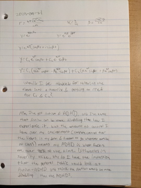
Transcript:

A number of calculations for a general solution for a linear second-order differential equation with constant coefficients. The assumption here is that for coefficients a, b, and c in the differential equation, b-squared is less than 4ac, resulting in complex roots for the quadratic. The root in the upper two quadrants of the Complex Plane is used to get constant coefficients alpha and beta, and then raising e to the power of alpha plus i times beta results in two solutions that solve the differential equation because of Euler's formula. The general solution and its first derivative are written with constant coefficients C1 and C2.

Would I be rebuked for throwing the above (the general solution and its derivative) into a matrix & getting to rref for C1 and C2?

Also, I've got Autism & ADHD, and I'm aware that Autism can be more disabling than how I experience it, but the amount of control I have over my environment (complete control over the lights in my dorm & freedom to go wherever outside of class) means my ADHD is what fucks me over 75% of the time. Differences in severity aside, why do I get the impression that the general public would look at Autism + ADHD and think the Autism would be more disabling than the ADHD?

[vvijaykumar]

https://answerkeyformath.com/higher-order-linear-differential-equations-i-ii-constant-coefficients/

AnswerkeyformathSolutionsforBscmathematicschapter5

[assignmenttutoronline]

程序代写案例-CHE452/ME452

ENGR452/BIOE452/CHE452/ME452 Instructor: Parisa Khodabakhshi Class 22 Review Topics for Test 2 Inhomogeneous linear ordinary differential equations. Method of undetermined coefficients for polynomial, trigonometric, and exponential forcing terms; cases when forcing term satis- fies homogeneous equation. Constant coefficient and Cauchy-Euler problems. Variation of parameters. Reduction of order…

[assignmentfreelancers]

程序代写案例-CHE452/ME452

ENGR452/BIOE452/CHE452/ME452 Instructor: Parisa Khodabakhshi Class 22 Review Topics for Test 2 Inhomogeneous linear ordinary differential equations. Method of undetermined coefficients for polynomial, trigonometric, and exponential forcing terms; cases when forcing term satis- fies homogeneous equation. Constant coefficient and Cauchy-Euler problems. Variation of parameters. Reduction of order…

[myassignmentonline]

程序代写案例-CHE452/ME452

ENGR452/BIOE452/CHE452/ME452 Instructor: Parisa Khodabakhshi Class 22 Review Topics for Test 2 Inhomogeneous linear ordinary differential equations. Method of undetermined coefficients for polynomial, trigonometric, and exponential forcing terms; cases when forcing term satis- fies homogeneous equation. Constant coefficient and Cauchy-Euler problems. Variation of parameters. Reduction of order…

[assignmenttutorsforyou]

程序代写案例-CHE452/ME452

ENGR452/BIOE452/CHE452/ME452 Instructor: Parisa Khodabakhshi Class 22 Review Topics for Test 2 Inhomogeneous linear ordinary differential equations. Method of undetermined coefficients for polynomial, trigonometric, and exponential forcing terms; cases when forcing term satis- fies homogeneous equation. Constant coefficient and Cauchy-Euler problems. Variation of parameters. Reduction of order…

[satyam-mathematics]

1.रैखिक समीकरण में रैखिक अवकल समीकरण (Linear Differential Equation in DE),अचर-गुणांकों वाले रैखिक अवकल समीकरण (Linear Differential Equations with Constant Coefficients):

रैखिक समीकरण में रैखिक अवकल समीकरण (Linear Differential Equation in DE) के इस आर्टिकल में अचर-गुणांकों वाले रैखिक अवकल समीकरणों का पूरक फलन तथा विशिष्ट समाकल ज्ञात करके व्यापक हल ज्ञात करना सीखेंगे।

Read More:Linear Differential Equation in DE

[goalrolli]

System of equation calculator

#System of equation calculator how to#

#System of equation calculator series#

Which method do you prefer?Ĭan you duplicate this? PTC Mathcad makes engineering calculations both easy and fun.

#System of equation calculator how to#

I especially recommend learning how to use Solve Blocks, as I have found them to be useful in many situations. By familiarizing yourself with these tools, you can apply them to a variety of engineering and math problems. Mathcad provides multiple methods for solving systems of equations. Now you have formulas for each of the variables. After selecting the solve keyword, type in a comma followed by the variables that you want to solve symbolically: We can do this using the Symbolic Evaluation operator and the solve keyword. Sometimes when we have a system of equations, instead of solving them numerically, we want to solve for the variables as functions of the coefficients or constants on the right-hand side of the expressions. You can also assign the lsolve function to a variable if desired. Evaluate the lsolve function using the matrix and the vector as the inputs.Create a vector of the constants appearing on the right-hand side of the system of equations.Create a matrix that contains the coefficients of the variables in your system of equations.To use lsolve, perform the following steps: Mathcad has a built-in function for solving a linear system of equations called lsolve. In a nonlinear system, one or more variables are raised to a power higher than one.Īlso, Mathcad will warn you if you have an inconsistent system of equations-that is, one for which a solution does not exist. A linear system is one in which the variables are all raised to the first power and the equation results in a line. I like Solve Blocks because they can be used to solve both linear and nonlinear systems of equations. Then outside of the Solve Block, evaluate the vector or individual variables to see the solutions. Then use the Definition operator to assign the Find function for the same variables. Solver: create a vector for the variables you want to solve for.Note that you use the Comparison operator, not the Evaluation operator, for the equals sign. Constraints: you write your system of equations here.If I have no idea what to use, I will use a value of 1. Guess Values: in this section, you initialize the variables that you want to solve for using the Definition operator to assign a value.The Solve Block is initiated from the Math tab. If you are going to use Mathcad for engineering calculations, I highly recommend you learn how to use this construct. In addition to solving systems of equations, it can be used to perform optimizations – finding the minimum or maximum for a function – and differential equations. The Solve Block is a special structure in Mathcad. where the constants (a,b,c and d) can be zero as long as. Let’s take a look at how to use each of these methods. A linear system of two equations with two variables is any system that can be written in the form. PTC Mathcad has a few methods that we can use to solve for the variables. Real-world examples that require solving a system of equations include Kirchhoff’s Law for electrical resistance and aerodynamic trajectories.

#System of equation calculator series#

In math and engineering, we often are left with a series of equations with an equal number of variables that we want to solve for.

[mathprofessorquotes]

Today we’ll be dealing with homogeneous constant coefficient second order linear differential equations, or as I prefer to call them, equations.

Differential Equations professor, Lancaster University

[musicallisto]

math has absolutely nothing to do with intelligence i can solve second order linear differential equations with non-constant coefficients but I've tried to understand inflation since 9th grade and i still don't fucking get it

[ask-the-path]

How are you enjoying "The Feynman Lectures on Physics"? What is a cool physics fact you learned from it that you would like to share with us?

Hi friend!!!

I enjoy all human books that I read!!

Right now I am on the chapter about the Harmonic Oscillator!! Which is perhaps the simplest mechanical system whose motion follows a linear differential equation with constant coefficients is a mass on a spring: first the spring stretches to balance the gravity; once it is balanced, we then discuss the vertical displacement of the mass from its equilibrium position. We shall call this upward displacement x, and we shall also suppose that the spring is perfectly linear, in which case the force pulling back when the spring is stretched is precisely proportional to the amount of stretch. That is, the force is −kx (with a minus sign to remind us that it pulls back). Thus the mass times the acceleration must equal −kx

Fun!!!

[vvijaykumar]

https://answerkeyformath.com/higher-order-linear-differential-equations-i-ii-constant-coefficients/

AnswerkeyformathSolutionsforBscmathematicschapter5