#Principal Component Analysis
Explore tagged Tumblr posts
Visit Tumblr Blog
Explore Tumblr blogs with no restrictions, modern design and the best experience.
Last Seen Tumblr Blogs


Fun Fact
Tumblr was attacked by a cross-site scripting worm deployed by the Internet troll group GNAA on Dec 3, 2012.
Text
Step-by-Step Guide to Principal Component Analysis (PCA)
A comprehensive guide to performing Principal Component Analysis (PCA). Follow the step-by-step process to understand how PCA reduces data dimensionality and aids in data visualization and analysis.
0 notes
Link
1 note
·
View note
Text
principal component analysis (PCA)
Dive into "What is Principal Component Analysis?" Simplify data intricacies, revealing key insights through effective dim

1 note
·
View note
Text
I think “alcohol and salads” is the funniest PCA-based dietary pattern, but I’m open to changing my mind. "Southern" is also kinda funny.
1 note
·
View note
Text
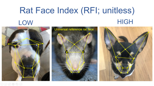
#courtesy of my functional ecology lecture#teaching us about principal component analysis#biology#zoology#ecology#ratblr#animal#dog#science
897 notes
·
View notes
Text
Reference archived on our website
TL;DR: 69.1% of people who've recovered from mild covid had lingering cognitive impairment.
Attempting to curb only severe acute disease opens us up to lingering post-viral illness that can be just as severe.
Abstract
Background:
Coronavirus disease 2019 (COVID-19) causes persistent symptoms, including brain fog. Based on limited research on the long-term consequences of mild COVID-19, which has yielded inconsistent results, we investigated which cognitive functions were most affected by COVID-19 in non-hospitalized Asian patients with long-term COVID and subjective cognitive complaints.
Methods:
Fifty-five non-hospitalized patients with long COVID and brain fog (24 males and 31 females, mean age: 45.6 ± 14.6 years, mean duration of education: 14.4 ± 3.0 years) were recruited. Neuropsychological assessments included screening tests for overall cognition, and comprehensive tests for memory, executive function, processing speed, and subjective emotional and disease symptoms. Cognitive test scores were converted into Z-scores. Moreover, principal component analysis (PCA) was employed to define cognitive domains across subtest scores.
Results:
Comprehensive assessments revealed cognitive impairment in 69.1% of patients (<1.5 standard deviation in at least one test). The processing speed (27.3%), memory recall (21.8%), memory learning (20.0%), and inhibitory control (18.2%) were the most affected areas. Self-reported anxiety and depression were observed in 35% and 33% of patients, respectively. Furthermore, the degree of self-anxiety can be used to predict learning performance.
Conclusion:
Nearly 70% of patients with subjective cognitive complaints and long COVID had objective cognitive impairments. A comprehensive evaluation is essential for patients with long COVID and brain fog, including those with mild symptoms.
#mask up#covid#pandemic#covid 19#wear a mask#public health#coronavirus#sars cov 2#still coviding#wear a respirator#long covid#covid conscious#covid is airborne
40 notes
·
View notes
Text


Found: first actively forming galaxy as lightweight as young Milky Way
For the first time, the NASA/ESA/CSA James Webb Space Telescope has detected and ‘weighed’ a galaxy that not only existed around 600 million years after the Big Bang, but also has a mass that is similar to what our Milky Way galaxy’s mass might have been at the same stage of development. Other galaxies Webb has detected at this period in the history of the Universe are significantly more massive. Nicknamed the Firefly Sparkle, this galaxy is gleaming with star clusters — 10 in all — each of which researchers examined in great detail.
“I didn’t think it would be possible to resolve a galaxy that existed so early in the Universe into so many distinct components, let alone find that its mass is similar to our own galaxy’s when it was in the process of forming,” said Lamiya Mowla, co-lead author of the paper and an assistant professor at Wellesley College in Massachusetts. “There is so much going on inside this tiny galaxy, including so many different phases of star formation.”
Webb was able to image the galaxy in sufficient detail for two reasons. One is a benefit of the cosmos: a massive foreground galaxy cluster radically enhanced the distant galaxy’s appearance through a natural effect known as gravitational lensing. And when combined with the telescope’s specialisation in high-resolution imaging of infrared light, Webb delivered unprecedented new data about the galaxy’s contents.
“Without the benefit of this gravitational lens, we would not be able to resolve this galaxy,” said Kartheik Iyer, co-lead author and NASA Hubble Fellow at Columbia University in New York. “We knew to expect it based on current physics, but it’s surprising that we actually saw it.”
Mowla, who spotted the galaxy in Webb’s image, was drawn to its gleaming star clusters, because objects that sparkle typically indicate they are extremely clumpy and complicated. Since the galaxy looks like a ‘sparkle’ or swarm of fireflies on a warm summer night, they named it the Firefly Sparkle galaxy.
Reconstructing the galaxy’s appearance
The research team modelled what the galaxy might have looked like if its image weren’t stretched by gravitational lensing and discovered that it resembled an elongated raindrop. Suspended within it are two star clusters toward the top and eight toward the bottom. “Our reconstruction shows that clumps of actively forming stars are surrounded by diffuse light from other unresolved stars,” said Iyer. “This galaxy is literally in the process of assembling.”
Webb’s data show the Firefly Sparkle galaxy is on the smaller side, falling into the category of a low-mass galaxy. Billions of years will pass before it builds its full heft and a distinct shape. “Most of the other galaxies Webb has shown us aren’t magnified or stretched, and we are not able to see their ‘building blocks’ separately. With Firefly Sparkle, we are witnessing a galaxy being assembled brick by brick,” Mowla said.
Stretched out and shining, ready for close analysis
Since the image of the galaxy is warped into a long arc, the researchers easily picked out 10 distinct star clusters, which are emitting the bulk of the galaxy’s light. They are represented here in shades of pink, purple, and blue. Those colours in Webb’s images and its supporting spectra confirmed that star formation didn’t happen all at once in this galaxy, but was staggered in time.
“This galaxy has a diverse population of star clusters, and it is remarkable that we can see them separately at such an early age of the Universe,” said Chris Willott of the National Research Council Canada, a co-author and the observation programme’s principal investigator. “Each clump of stars is undergoing a different phase of formation or evolution.”
The galaxy’s projected shape shows that its stars haven’t settled into a central bulge or a thin, flattened disc, another piece of evidence that the galaxy is still forming.
‘Glowing’ companions
Researchers can’t predict how this disorganised galaxy will build up and take shape over billions of years, but there are two galaxies that the team confirmed are ‘hanging out’ within a tight perimeter and may influence how it builds mass over billions of years.
Firefly Sparkle is only 6500 light-years away from its first companion, and its second companion is separated by 42 000 light-years. For context, the fully formed Milky Way is about 100 000 light-years across — all three would fit inside it. Not only are its companions very close, the researchers also think that they are orbiting one another.
Each time one galaxy passes another, gas condenses and cools, allowing new stars to form in clumps, adding to the galaxies’ masses. “It has long been predicted that galaxies in the early Universe form through successive interactions and mergers with other tinier galaxies,” said Yoshihisa Asada, a co-author and doctoral student at Kyoto University in Japan. “We might be witnessing this process in action.”
“This is just the first of many such galaxies JWST will discover, as we are only starting to use these cosmic microscopes”, added team member Maruša Bradač of the University of Ljubljana in Slovenia. “Just like microscopes let us see pollen grains from plants, the incredible resolution of Webb and the magnifying power of gravitational lensing let us see the small pieces inside galaxies. Our team is now analysing all early galaxies, and the results are all pointing in the same direction: we have yet to learn much more about how those early galaxies formed.”
The team’s research relied on data from Webb’s CAnadian NIRISS Unbiased Cluster Survey, which include near-infrared images from NIRCam (Near-InfraRed Camera) and spectra from the microshutter array aboard NIRSpec (Near-Infrared Spectrograph). The CANUCS data intentionally covered a field that NASA’s Hubble Space Telescope imaged as part of its Cluster Lensing And Supernova survey with Hubble programme.
This work was published on 12 December 2024 in the journal Nature.
More information
Webb is the largest, most powerful telescope ever launched into space. Under an international collaboration agreement, ESA provided the telescope’s launch service, using the Ariane 5 launch vehicle. Working with partners, ESA was responsible for the development and qualification of Ariane 5 adaptations for the Webb mission and for the procurement of the launch service by Arianespace. ESA also provided the workhorse spectrograph NIRSpec and 50% of the mid-infrared instrument MIRI, which was designed and built by a consortium of nationally funded European Institutes (The MIRI European Consortium) in partnership with JPL and the University of Arizona.
Webb is an international partnership between NASA, ESA and the Canadian Space Agency (CSA).
Image Credit: NASA, ESA, CSA, STScI, C. Willott (NRC-Canada), L. Mowla (Wellesley College), K. Iyer (Columbia)
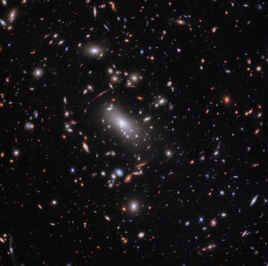
TOP IMAGE: Thousands of glimmering galaxies are bound together by their own gravity, making up a massive cluster formally classified as MACS J1423.
The largest bright white oval is a supergiant elliptical galaxy that is the dominant member of this galaxy cluster. The galaxy cluster acts like a lens, magnifying and distorting the light from objects that lie well behind it, an effect known as gravitational lensing that has big research benefits. Astronomers can study lensed galaxies in detail, like the Firefly Sparkle galaxy.
This 2023 image is from the James Webb Space Telescope’s NIRCam (Near-InfraRed Camera). Researchers used Webb to survey the same field that the Hubble Space Telescope imaged in 2010. Thanks to its specialisation in high-resolution near-infrared imagery, Webb was able to show researchers many more galaxies in far more detail.
[Image description: Thousands of overlapping objects at various distances are spread across this field, including galaxies in a massive galaxy cluster, and distorted background galaxies behind the galaxy cluster. The background of space is black.]Credit:
NASA, ESA, CSA, STScI, C. Willott (NRC-Canada), L. Mowla (Wellesley College), K. Iyer (Columbia)
CENTRE IMAGE: For the first time, astronomers have identified a still-forming galaxy that weighs about the same as our Milky Way if we could wind back the clock to see our galaxy as it developed. The newly identified galaxy, the Firefly Sparkle, is in the process of assembling and forming stars, and existed about 600 million years after the Big Bang.
The image of the galaxy is stretched and warped by a natural effect known as gravitational lensing, which allowed researchers to glean far more information about its contents. (In some areas of Webb’s image, the galaxy is magnified over 40 times.)
While it took shape, the galaxy gleamed with star clusters in a range of infrared colours, which are scientifically meaningful. They indicate that the stars formed at different periods, not all at once.
Since the galaxy image is stretched into a long line in Webb’s observations, researchers were able to identify 10 distinct star clusters and study them individually, along with the cocoon of diffuse light from the additional, unresolved stars surrounding them. That’s not always possible for distant galaxies that aren’t lensed. Instead, in many cases researchers can only draw conclusions that apply to an entire galaxy. “Most of the other galaxies Webb has shown us aren’t magnified or stretched and we are not able to see the ‘building blocks’ separately. With Firefly Sparkle, we are witnessing a galaxy being assembled brick by brick,” explains astronomer Lamiya Mowla.
There are two companion galaxies ‘hovering’ close by, which may ultimately affect how this galaxy forms and builds mass over billions of years. Firefly Sparkle is only about 6500 light-years away from its first companion, and 42 000 light-years from its second companion. Let’s compare these figures to objects that are closer to home: the Sun is about 26 000 light-years from the centre of our Milky Way galaxy, and the Milky Way is about 100 000 light-years across. Not only are Firefly Sparkle’s companions very close, the researchers also suspect that they are orbiting one another.
[Image description: Horizontal split down the middle. At left, thousands of overlapping objects at various distances are spread across this galaxy cluster. A box at bottom right is enlarged on the right half. A central oval identifies the Firefly Sparkle galaxy, a line with 10 dots in various colours.]Credit:
NASA, ESA, CSA, STScI, C. Willott (NRC-Canada), L. Mowla (Wellesley College), K. Iyer (Columbia)
LOWER IMAGE: Thousands of glimmering galaxies are bound together by their own gravity, making up a massive cluster formally classified as MACS J1423.
The largest bright white oval is a supergiant elliptical galaxy that is the dominant member of this galaxy cluster. The galaxy cluster acts like a lens, magnifying and distorting the light from objects that lie well behind it, an effect known as gravitational lensing that has big research benefits. Astronomers can study lensed galaxies in detail, like the Firefly Sparkle galaxy.
This 2023 image is from the James Webb Space Telescope’s NIRCam (Near-Infrared Camera). Researchers used Webb to survey the same field the Hubble Space Telescope imaged in 2010. Thanks to its specialisation in high-resolution near-infrared imagery, Webb was able to show researchers many more galaxies in far more detail.
The north and east compass arrows show the orientation of the image on the sky.
The scale bar is labelled in arcseconds, which is a measure of angular distance on the sky. One arcsecond is equal to an angular measurement of 1/3600 of one degree. There are 60 arcminutes in a degree and 60 arcseconds in an arcminute. (The full Moon has an angular diameter of about 30 arcminutes.) The actual size of an object that covers one arcsecond on the sky depends on its distance from the telescope.
This image shows invisible near-infrared wavelengths of light that have been translated into visible-light colours. The colour key shows which NIRCam filters were used when collecting the light. The colour of each filter name is the visible light colour used to represent the infrared light that passes through that filter.
NIRCam filters from left to right: F115W and F150W are blue; F200W and F277W are green; F356W and F444W are red.
[Image description: A graphic labelled “James Webb Space Telescope; MACS J1423.8+2404.” A rectangular image shows thousands of galaxies of various shapes and colours on the black background of space.]Credit:
NASA, ESA, CSA, STScI, C. Willott (NRC-Canada), L. Mowla (Wellesley College), K. Iyer (Columbia)
youtube
9 notes
·
View notes
Text

february 1st, 2024
one thing i was hoping to learn during my post-bac but never really got around to was spike sorting. in my neural engineering class, i'm finally learning how to do that!
although i don't plan on collecting neural data at this level, i do hope to collect LFPs as part of my research so learning this signal processing in general is going to be extremely helpful. so far, i've determined my threshold and plotted the threshold line within the data. the hard part is everything that comes next of template matching, principal component analysis (PCA), and all the like. after not really using MATLAB in yeeears, this has been an adventure but i'm surprised at how much i've been able to recall and proud of myself for having no shame in googling MATLAB functions lol. i know i can figure this out, i'm smart(ish).
this hw is due feb 7th (with possibility of an extension if other people in the class take a while) so time to get her done. ft my pupper knocked out on the floor
#alexistudies#alexi's phd year 1#studyblr#matlab#biomedical engineering#engblr#gradblr#phdblr#phd life#grad student#study aesthetic#studyspo#genspen#hey gen#morningkou#stemblr#scienceblr#collegeblr#uniblr#study blog#study motivation#student life#studying#learning#learnign#elkstudies#studyingchemeng#selkiestudies
48 notes
·
View notes
Text
K-2 and K-4 Visas
The K-2 and K-4 visas are non-immigrant visa categories that allow eligible children of U.S. fiancé(e) or spouse visa applicants to enter the United States and accompany their parent pending adjustment of status to lawful permanent resident (Green Card holder). These visa types are critical components of family unification under U.S. immigration law, offering minor children lawful admission rights linked to their parent’s K-1 (fiancé(e)) or K-3 (spouse) visa application.
For Thai nationals, understanding the nuanced legal framework and procedural requirements behind the K-2 and K-4 visa processes is essential, especially when navigating consular processing at the U.S. Embassy in Bangkok or the U.S. Consulate General in Chiang Mai.
This article provides a comprehensive, legal, and procedural analysis of the K-2 and K-4 visa pathways from Thailand, highlighting eligibility rules, documentary requirements, application steps, and strategic pitfalls to avoid.
1. Legal Basis and U.S. Immigration Framework
1.1 Governing Laws
Immigration and Nationality Act (INA) § 101(a)(15)(K): Defines K visa classifications
8 CFR § 214.2(k): Regulatory guidance for K-2 and K-4 visa procedures
Department of State Foreign Affairs Manual (FAM): Consular officer guidelines for adjudicating K visas
1.2 Purpose of K-2 and K-4 Visas
K-2 Visa: For unmarried children under 21 years old of a K-1 fiancé(e) visa holder.
K-4 Visa: For unmarried children under 21 years old of a K-3 spouse visa holder.
Both allow children to travel to the U.S. alongside or after the principal visa holder and apply for adjustment of status to become lawful permanent residents once the parent marries (in K-1 cases) or completes immigrant visa processing (in K-3 cases).
Important: Stepchildren of U.S. citizens applying for K-4 visas must establish that the marriage between the U.S. citizen and the foreign spouse occurred before the child's 18th birthday under U.S. immigration law.
2. Procedural Steps for Thai Applicants
3.1 K-2 Visa Linked to K-1 Parent (Fiancé(e))
Form I-129F Petition: U.S. citizen fiancé(e) must list child(ren) on the petition.
USCIS Approval: Petition sent to the National Visa Center (NVC) for processing.
Consular Processing:
Apply separately for each K-2 child through DS-160 forms.
Schedule a visa interview at the U.S. Embassy Bangkok or U.S. Consulate Chiang Mai.
Medical Exam: Conducted at an approved clinic.
Interview and Visa Issuance:
Child’s eligibility is separately assessed.
Parent and child may be interviewed together or separately.
Entry into the U.S.: Child enters with K-2 visa.
Adjustment of Status: File Form I-485 after parent's marriage to U.S. citizen within 90 days.
2.2 K-4 Visa Linked to K-3 Parent (Spouse)
Form I-130 and Form I-129F Petitions: U.S. citizen files both petitions for the foreign spouse.
K-3 Approval: Visa processing through NVC.
K-4 Visa Application:
No separate petition required for child if marriage occurred before the child’s 18th birthday.
Complete DS-160 application.
Medical Exam and Interview.
Entry into the U.S.: K-4 child accompanies parent.
Adjustment of Status: File Form I-485 once the immigrant petition (I-130) is approved.
Thai birth certificates and legal documents must be translated into English and certified.
3. Important Legal and Practical Considerations
3.1 Age-Out Risks
A child must enter the U.S. while still under 21 years of age.
The Child Status Protection Act (CSPA) may offer limited protection by "freezing" the child's age, but K-2/K-4 beneficiaries must generally act quickly.
3.2 Adjustment of Status Timing
K-2 child must apply for adjustment of status after the principal K-1 holder marries the U.S. citizen.
K-4 child must adjust status after the approval of the immigrant petition (I-130).
3.3 Separate Applications
Children must file separate Form I-485s when adjusting status—there is no automatic derivation based on parent’s adjustment.
3.4 Work and Travel Authorization
K-2 and K-4 visa holders may apply for:
Employment Authorization Document (EAD) by filing Form I-765.
Advance Parole for travel outside the U.S. while the adjustment application is pending.
4. Consular Processing at U.S. Embassy Bangkok / Consulate Chiang Mai
High scrutiny of family relationship authenticity.
Officers may require original birth certificates, proof of continuous relationship, and even school records.
K-2 and K-4 children must be prepared for basic questions at interviews about:
Family circumstances
Relationship to U.S. sponsor
Intent to reside in the U.S. with parent
Costs for biometrics, translations, and courier services are additional.
5. Conclusion
The K-2 and K-4 visas offer essential immigration pathways for minor children to reunite with their parents in the United States under the family-based immigration system. However, they require careful coordination between the K-1/K-3 process, Thai document standards, and U.S. immigration timelines, especially given the strict age and marital status restrictions.
For Thai applicants, successful outcomes depend on meticulous documentary preparation, attention to procedural deadlines, and a clear understanding of the parent-child relationship requirements. Failure to align the timelines correctly or prepare adequate documentation can result in severe setbacks, including visa refusal or aging out of eligibility.
3 notes
·
View notes
Text
Born to smoke weed, forced to do principal component analysis </3
2 notes
·
View notes
Text
Understanding Principal Component Analysis (PCA)

The world of data is vast and complex. Machine Learning thrives on this data, but with great power comes great responsibility (to manage all those features!). This is where Principal Component Analysis (PCA) steps in, offering a powerful technique for simplifying complex datasets in Machine Learning.
What is Principal Component Analysis?
Imagine a room filled with clothes. Each piece of clothing represents a feature in your data. PCA helps you organize this room by identifying the most important categories (like shirts, pants, dresses) and arranging them efficiently.
It does this by transforming your data into a lower-dimensional space while capturing the most significant information. This not only simplifies analysis but also improves the performance of Machine Learning algorithms.
Fundamentals of Principal Component Analysis (PCA)
At its core, Principal Component Analysis (PCA) is a technique used in Machine Learning for dimensionality reduction. Imagine a room filled with clothes, each piece representing a feature in your data.
PCA helps organize this room by identifying the most important categories (like shirts, pants, dresses) and arranging them efficiently in a smaller space. Here’s a breakdown of the fundamental steps involved in PCA:
Standardization
PCA assumes your data is centered around a mean of zero and has equal variances. Standardization ensures this by subtracting the mean from each feature and scaling them to have a unit variance. This creates a level playing field for all features, preventing biases due to different scales.
Covariance Matrix
This matrix captures the relationships between all features in your data. A high covariance value between two features indicates they tend to move together (e.g., height and weight). Conversely, a low covariance suggests they are relatively independent.
Eigenvectors and Eigenvalues
PCA finds a set of directions (eigenvectors) that explain the most variance in your data. Each eigenvector is associated with an eigenvalue, which represents the proportion of variance it captures.
Think of eigenvectors as new axes along which your data can be arranged, and eigenvalues as measures of how “important” those axes are in capturing the spread of your data points.
Component Selection
You choose the most informative eigenvectors (based on their corresponding eigenvalues) to create your new, lower-dimensional space. These eigenvectors are often referred to as “principal components” because they capture the essence of your original data.
By selecting the top eigenvectors with the highest eigenvalues, you retain the most important variations in your data while discarding less significant ones.
Understanding these fundamentals is crucial for effectively using PCA in your Machine Learning projects. It allows you to interpret the results and make informed decisions about the number of components to retain for optimal performance.
Applications of PCA in Machine Learning
PCA is a versatile tool with a wide range of applications:
Dimensionality Reduction
As mentioned earlier, PCA helps reduce the number of features in your data, making it easier to visualize, analyze, and use in Machine Learning models.
Feature Engineering
PCA creates new, uncorrelated features (principal components) that can be more informative than the originals for specific tasks.
Anomaly Detection
By identifying patterns in the principal components, PCA can help you detect outliers and unusual data points.
Image Compression
PCA plays a role in compressing images by discarding less important components, reducing file size without significant visual degradation.
Recommendation Systems
PCA can be used to analyze user preferences and recommend relevant products or services based on underlying patterns.
Implementing PCA in Machine Learning Projects
While the core concepts of PCA are crucial, its real power lies in its practical application. This section dives into how to implement PCA in your Machine Learning projects using Python libraries like Scikit-learn.
Prerequisites
Basic understanding of Python programming
Familiarity with Machine Learning concepts
Libraries
We’ll be using the following libraries:
Pandas: Data manipulation
Numpy: Numerical computations
Scikit-learn: Machine Learning algorithms (specifically PCA from decomposition)
Note: Make sure you have these libraries installed using pip install pandas, numpy, scikit-learn.
Sample Dataset
Let’s consider a dataset with customer information, including features like age, income, spending habits (various categories), and location. We want to use PCA to reduce dimensionality before feeding the data into a recommendation system.
Step 1: Import libraries and data

Step 2: Separate features and target (optional)
In this example, we’re focusing on dimensionality reduction, so we don’t necessarily need a target variable. However, if your task involves prediction, separate the features (explanatory variables) and target variable.

Step 3: Standardize the data
PCA is sensitive to the scale of features. Standardize the data using StandardScaler from scikit-learn.

Step 4: Create the PCA object
Instantiate a PCA object, specifying the desired number of components (we’ll discuss this later) or leaving it blank for an initial analysis.

Step 5: Fit the PCA model
Train the PCA model on the standardized features.

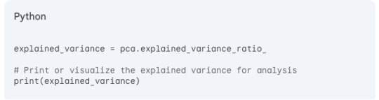
Step 6: Analyze explained variance
PCA outputs the explained variance ratio (explained_variance_ratio_) for each principal component. This represents the proportion of variance captured by that component.
Step 7: Choose the number of components (n_components)
Here’s the crux of PCA implementation. You need to decide how many principal components to retain. There’s no single answer, but consider these factors:
Explained variance: Aim for components that capture a significant portion of the total variance (e.g., 80–90%).
Information loss: Retaining too few components might discard valuable information.
Model complexity: Using too many components might increase model complexity without significant benefit.
A common approach is to iteratively fit PCA models with different n_components and analyze the explained variance. You can also use tools like the scree plot to visualize the “elbow” where the explained variance plateaus.
Step 8: Transform the data
Once you’ve chosen the number of components, create a new PCA object with that specific value and transform the data into the principal component space.

Note: The transformed_data now contains your data projected onto the new, lower-dimensional space defined by the principal components.
Step 9: Use the transformed data
You can now use the transformed_data for further analysis or train your machine learning model with these reduced features.
Additional Tips:
Explore visualization techniques like plotting the principal components to understand the underlying structure of your data.
Remember that PCA assumes linear relationships between features. If your data exhibits non-linearity, consider alternative dimensionality reduction techniques.
By following these steps, you can effectively implement PCA in your machine learning projects to unlock the benefits of dimensionality reduction and enhance your models’ performance.
Frequently Asked Questions
How Much Dimensionality Reduction is Too Much?
There’s no one-size-fits-all answer. It depends on your data and the information you want to retain. Evaluation metrics can help you determine the optimal number of components.
Can PCA Handle Non-linear Relationships?
No, PCA works best with linear relationships between features. For non-linear data, consider alternative dimensionality reduction techniques.
Does PCA Improve Model Accuracy?
Not always directly. However, by simplifying data and reducing noise, PCA can often lead to better performing Machine Learning models.
Conclusion
PCA is a powerful tool that simplifies complex data, making it a valuable asset in your Machine Learning toolkit. By understanding its core concepts and applications, you can leverage PCA to unlock insights and enhance the performance of your Machine Learning projects.
Ready to take your Machine Learning journey further?
Enrol in our free introductory course on Machine Learning Fundamentals! Learn the basics, explore various algorithms, and unlock the potential of data in your projects.
0 notes
Text
Machine Learning: A Comprehensive Overview
Machine Learning (ML) is a subfield of synthetic intelligence (AI) that offers structures with the capacity to robotically examine and enhance from revel in without being explicitly programmed. Instead of using a fixed set of guidelines or commands, device studying algorithms perceive styles in facts and use the ones styles to make predictions or decisions. Over the beyond decade, ML has transformed how we have interaction with generation, touching nearly each aspect of our every day lives — from personalised recommendations on streaming services to actual-time fraud detection in banking.

Machine learning algorithms
What is Machine Learning?
At its center, gadget learning entails feeding facts right into a pc algorithm that allows the gadget to adjust its parameters and improve its overall performance on a project through the years. The more statistics the machine sees, the better it usually turns into. This is corresponding to how humans study — through trial, error, and revel in.
Arthur Samuel, a pioneer within the discipline, defined gadget gaining knowledge of in 1959 as “a discipline of take a look at that offers computers the capability to study without being explicitly programmed.” Today, ML is a critical technology powering a huge array of packages in enterprise, healthcare, science, and enjoyment.
Types of Machine Learning
Machine studying can be broadly categorised into 4 major categories:
1. Supervised Learning
For example, in a spam electronic mail detection device, emails are classified as "spam" or "no longer unsolicited mail," and the algorithm learns to classify new emails for this reason.
Common algorithms include:
Linear Regression
Logistic Regression
Support Vector Machines (SVM)
Decision Trees
Random Forests
Neural Networks
2. Unsupervised Learning
Unsupervised mastering offers with unlabeled information. Clustering and association are commonplace obligations on this class.
Key strategies encompass:
K-Means Clustering
Hierarchical Clustering
Principal Component Analysis (PCA)
Autoencoders
three. Semi-Supervised Learning
It is specifically beneficial when acquiring categorised data is highly-priced or time-consuming, as in scientific diagnosis.
Four. Reinforcement Learning
Reinforcement mastering includes an agent that interacts with an surroundings and learns to make choices with the aid of receiving rewards or consequences. It is broadly utilized in areas like robotics, recreation gambling (e.G., AlphaGo), and independent vehicles.
Popular algorithms encompass:
Q-Learning
Deep Q-Networks (DQN)
Policy Gradient Methods
Key Components of Machine Learning Systems
1. Data
Data is the muse of any machine learning version. The pleasant and quantity of the facts directly effect the performance of the version. Preprocessing — consisting of cleansing, normalization, and transformation — is vital to make sure beneficial insights can be extracted.
2. Features
Feature engineering, the technique of selecting and reworking variables to enhance model accuracy, is one of the most important steps within the ML workflow.
Three. Algorithms
Algorithms define the rules and mathematical fashions that help machines study from information. Choosing the proper set of rules relies upon at the trouble, the records, and the desired accuracy and interpretability.
4. Model Evaluation
Models are evaluated the use of numerous metrics along with accuracy, precision, consider, F1-score (for class), or RMSE and R² (for regression). Cross-validation enables check how nicely a model generalizes to unseen statistics.
Applications of Machine Learning
Machine getting to know is now deeply incorporated into severa domain names, together with:
1. Healthcare
ML is used for disorder prognosis, drug discovery, customized medicinal drug, and clinical imaging. Algorithms assist locate situations like cancer and diabetes from clinical facts and scans.
2. Finance
Fraud detection, algorithmic buying and selling, credit score scoring, and client segmentation are pushed with the aid of machine gaining knowledge of within the financial area.
3. Retail and E-commerce
Recommendation engines, stock management, dynamic pricing, and sentiment evaluation assist businesses boom sales and improve patron revel in.
Four. Transportation
Self-riding motors, traffic prediction, and route optimization all rely upon real-time gadget getting to know models.
6. Cybersecurity
Anomaly detection algorithms help in identifying suspicious activities and capacity cyber threats.
Challenges in Machine Learning
Despite its rapid development, machine mastering still faces numerous demanding situations:
1. Data Quality and Quantity
Accessing fantastic, categorised statistics is often a bottleneck. Incomplete, imbalanced, or biased datasets can cause misguided fashions.
2. Overfitting and Underfitting
Overfitting occurs when the model learns the education statistics too nicely and fails to generalize.
Three. Interpretability
Many modern fashions, specifically deep neural networks, act as "black boxes," making it tough to recognize how predictions are made — a concern in excessive-stakes regions like healthcare and law.
4. Ethical and Fairness Issues
Algorithms can inadvertently study and enlarge biases gift inside the training facts. Ensuring equity, transparency, and duty in ML structures is a growing area of studies.
5. Security
Adversarial assaults — in which small changes to enter information can fool ML models — present critical dangers, especially in applications like facial reputation and autonomous riding.
Future of Machine Learning
The destiny of system studying is each interesting and complicated. Some promising instructions consist of:
1. Explainable AI (XAI)
Efforts are underway to make ML models greater obvious and understandable, allowing customers to believe and interpret decisions made through algorithms.
2. Automated Machine Learning (AutoML)
AutoML aims to automate the stop-to-cease manner of applying ML to real-world issues, making it extra reachable to non-professionals.
3. Federated Learning
This approach permits fashions to gain knowledge of across a couple of gadgets or servers with out sharing uncooked records, enhancing privateness and efficiency.
4. Edge ML
Deploying device mastering models on side devices like smartphones and IoT devices permits real-time processing with reduced latency and value.
Five. Integration with Other Technologies
ML will maintain to converge with fields like blockchain, quantum computing, and augmented fact, growing new opportunities and challenges.
2 notes
·
View notes
Text
The Science Behind Effective Disease Management in Trees
Trees are usually not just principal formula of our ecosystems; they are also living entities that require care and leadership, noticeably with regards to ailment prevention and healing. Understanding the science in the back of tremendous disorder leadership in trees is the most important for arborists, tree service specialists, and owners alike. This article delves into the complicated data of tree health and wellbeing administration, presenting insights, recommendations, and proven procedures to make sure that your timber stay bright and resilient.

Understanding Tree Diseases: An Overview What Are Tree Diseases?
Tree sicknesses might be labeled broadly into two varieties: infectious illnesses as a result of pathogens (fungi, micro organism, viruses) and non-infectious ailments attributable to environmental components (nutrient deficiencies, mechanical injuries).
The Role of Pathogens
Infectious sicknesses are steadily spread due to spores or contact with infected supplies. For illustration:
Fungal Infections: These can lead to troubles like root rot or leaf blight. Bacterial Infections: Often rationale wilting or cankers on branches.
Understanding those pathogens is needed for imposing the accurate techniques in handling tree healthiness.
Non-Infectious Factors
On any other hand, non-infectious motives can consist of:
Poor soil high quality. Water stress (either too much or too little). Physical break as a consequence of storms or human routine.
Recognizing the signs and symptoms of both sorts of illnesses is a very important first step in beneficial disease control.

The Science Behind Effective Disease Management in Trees
Effective disease management hinges on a scientific realizing of the way bushes have interaction with their ecosystem. This involves recognizing disorder signs and symptoms early and knowing how one can reply accurately.
youtube
Symptoms of Tree Diseases
Identifying warning signs as early as a possibility is vital to superb management. Common signals embrace:
Wilting leaves Discoloration (yellowing or browning) Abnormal boom patterns
By monitoring these warning signs repeatedly, you might take proactive measures prior to a minor subject escalates into a first-rate limitation.
Diagnosis Techniques
Utilizing progressive diagnostic methods can considerably escalate your capacity to deal with http://hdztreeservicesinc.com/ tree illnesses without problems. Some systems include:
Visual Inspection: Regular checks for indications of misery. Soil Testing: To settle on nutrient tiers and discover deficiencies. Laboratory Analysis: Sending samples for professional exam when integral. Preventive Measures for Tree Health
Preventive measures type the backbone of any valuable disorder control method. Here’s how you could possibly put in force them:
youtube
Proper Planting Techniques
Planting bushes successfully sets them up for good fortune from the beginning. Essential advice contain:
Ensuring enough spacing betw
2 notes
·
View notes
Text

A Beginner's Guide to Principal Component Analysis (PCA) in Data Science and Machine Learning
Principal Component Analysis (PCA) is one of the most important techniques for dimensionality reduction in machine learning and data science. It allows us to simplify datasets, making them easier to work with while retaining as much valuable information as possible. PCA has become a go-to method for preprocessing high-dimensional data.
Click here to read more
#artificial intelligence#bigdata#books#machine learning#machinelearning#programming#python#science#skills#big data
3 notes
·
View notes
Text

Genetic diagram of citrus
Three-dimensional projection of a principal component analysis of citrus hybrids, with citron (yellow), pomelo (blue), mandarin (red), and micrantha (green) defining the axes. Hybrids are expected to plot between their parents. ML: 'Mexican' lime; A: 'Alemow'; V: 'Volkamer' lemon; M: 'Meyer' lemon; L: Regular and 'Sweet' lemons; B: Bergamot orange; H: Haploid clementine; C: Clementines; S: Sour oranges; O: Sweet oranges; G: Grapefruits. Figure from Curk, et al. (2014).
4 notes
·
View notes
Text
Reference preserved on our archive (Check us out for daily updates!)
Highlights •Placental response to SARS-CoV-2-infection and timing of infection is unclear. •Inflammatory and cardiovascular proteins were analysed in 103 placentas. •Protein levels were unchanged regardless of timing of SARS-CoV-2-infection. •Future studies are needed on placental changes depending on severity of infection.
Abstract Introduction Maternal SARS-CoV-2 infection can affect pregnancy outcome, but the placental response to and the effect of timing of infection is not well studied. The aim of this study was to investigate the placental levels of inflammatory and cardiovascular markers in pregnancies complicated by SARS-CoV-2 infection compared to non-infected pregnancies, and to investigate whether there was an association between time point of infection during pregnancy and placental inflammatory and cardiovascular protein levels.
Methods Placental samples from a prospectively recruited pregnancy cohort of SARS-CoV-2-infected (n = 53) and non-infected (n = 50) women were analysed for 177 inflammatory and cardiovascular proteins, using an antibody-based proximity extension assay. In the SARS-CoV-2-infected group, half of the women were infected before 20 weeks of gestation, and five women were hospitalised for severe SARS-CoV-2 infection. Single-protein analyses were performed with linear mixed effects models, followed by Benjamini-Hochberg correction for multiple testing. Multi-protein analyses were performed using principal component analysis and machine learning algorithms.
Results The perinatal outcomes and the placental levels of inflammatory or cardiovascular proteins in women with SARS-CoV-2 infection were similar to those in non-infected women. There were no differences in inflammatory or cardiovascular protein levels between early and late pregnancy SARS-CoV-2 infection, nor any linear correlations between protein levels and gestational age at time of infection.
Discussion Women with SARS-CoV-2 infection during pregnancy without clinical signs of placental insufficiency have no changes in inflammatory or cardiovascular protein patterns in placenta at time of birth regardless of the timing of the infection.
#mask up#covid#pandemic#public health#covid 19#wear a mask#wear a respirator#still coviding#coronavirus#sars cov 2#covid in pregnancy
19 notes
·
View notes