#explain DFS algorithm | Explore Tumblr posts and blogs

simerjeet · 6 months ago

Text

Mastering Data Structures: A Comprehensive Course for Beginners

Data structures are one of the foundational concepts in computer science and software development. Mastering data structures is essential for anyone looking to pursue a career in programming, software engineering, or computer science. This article will explore the importance of a Data Structure Course, what it covers, and how it can help you excel in coding challenges and interviews.

1. What Is a Data Structure Course?

A Data Structure Course teaches students about the various ways data can be organized, stored, and manipulated efficiently. These structures are crucial for solving complex problems and optimizing the performance of applications. The course generally covers theoretical concepts along with practical applications using programming languages like C++, Java, or Python.

By the end of the course, students will gain proficiency in selecting the right data structure for different problem types, improving their problem-solving abilities.

2. Why Take a Data Structure Course?

Learning data structures is vital for both beginners and experienced developers. Here are some key reasons to enroll in a Data Structure Course:

a) Essential for Coding Interviews

Companies like Google, Amazon, and Facebook focus heavily on data structures in their coding interviews. A solid understanding of data structures is essential to pass these interviews successfully. Employers assess your problem-solving skills, and your knowledge of data structures can set you apart from other candidates.

b) Improves Problem-Solving Skills

With the right data structure knowledge, you can solve real-world problems more efficiently. A well-designed data structure leads to faster algorithms, which is critical when handling large datasets or working on performance-sensitive applications.

c) Boosts Programming Competency

A good grasp of data structures makes coding more intuitive. Whether you are developing an app, building a website, or working on software tools, understanding how to work with different data structures will help you write clean and efficient code.

3. Key Topics Covered in a Data Structure Course

A Data Structure Course typically spans a range of topics designed to teach students how to use and implement different structures. Below are some key topics you will encounter:

a) Arrays and Linked Lists

Arrays are one of the most basic data structures. A Data Structure Course will teach you how to use arrays for storing and accessing data in contiguous memory locations. Linked lists, on the other hand, involve nodes that hold data and pointers to the next node. Students will learn the differences, advantages, and disadvantages of both structures.

b) Stacks and Queues

Stacks and queues are fundamental data structures used to store and retrieve data in a specific order. A Data Structure Course will cover the LIFO (Last In, First Out) principle for stacks and FIFO (First In, First Out) for queues, explaining their use in various algorithms and applications like web browsers and task scheduling.

c) Trees and Graphs

Trees and graphs are hierarchical structures used in organizing data. A Data Structure Course teaches how trees, such as binary trees, binary search trees (BST), and AVL trees, are used in organizing hierarchical data. Graphs are important for representing relationships between entities, such as in social networks, and are used in algorithms like Dijkstra's and BFS/DFS.

d) Hashing

Hashing is a technique used to convert a given key into an index in an array. A Data Structure Course will cover hash tables, hash maps, and collision resolution techniques, which are crucial for fast data retrieval and manipulation.

e) Sorting and Searching Algorithms

Sorting and searching are essential operations for working with data. A Data Structure Course provides a detailed study of algorithms like quicksort, merge sort, and binary search. Understanding these algorithms and how they interact with data structures can help you optimize solutions to various problems.

4. Practical Benefits of Enrolling in a Data Structure Course

a) Hands-on Experience

A Data Structure Course typically includes plenty of coding exercises, allowing students to implement data structures and algorithms from scratch. This hands-on experience is invaluable when applying concepts to real-world problems.

b) Critical Thinking and Efficiency

Data structures are all about optimizing efficiency. By learning the most effective ways to store and manipulate data, students improve their critical thinking skills, which are essential in programming. Selecting the right data structure for a problem can drastically reduce time and space complexity.

c) Better Understanding of Memory Management

Understanding how data is stored and accessed in memory is crucial for writing efficient code. A Data Structure Course will help you gain insights into memory management, pointers, and references, which are important concepts, especially in languages like C and C++.

5. Best Programming Languages for Data Structure Courses

While many programming languages can be used to teach data structures, some are particularly well-suited due to their memory management capabilities and ease of implementation. Some popular programming languages used in Data Structure Courses include:

C++: Offers low-level memory management and is perfect for teaching data structures.

Java: Widely used for teaching object-oriented principles and offers a rich set of libraries for implementing data structures.

Python: Known for its simplicity and ease of use, Python is great for beginners, though it may not offer the same level of control over memory as C++.

6. How to Choose the Right Data Structure Course?

Selecting the right Data Structure Course depends on several factors such as your learning goals, background, and preferred learning style. Consider the following when choosing:

a) Course Content and Curriculum

Make sure the course covers the topics you are interested in and aligns with your learning objectives. A comprehensive Data Structure Course should provide a balance between theory and practical coding exercises.

b) Instructor Expertise

Look for courses taught by experienced instructors who have a solid background in computer science and software development.

c) Course Reviews and Ratings

Reviews and ratings from other students can provide valuable insights into the course’s quality and how well it prepares you for real-world applications.

7. Conclusion: Unlock Your Coding Potential with a Data Structure Course

In conclusion, a Data Structure Course is an essential investment for anyone serious about pursuing a career in software development or computer science. It equips you with the tools and skills to optimize your code, solve problems more efficiently, and excel in technical interviews. Whether you're a beginner or looking to strengthen your existing knowledge, a well-structured course can help you unlock your full coding potential.

By mastering data structures, you are not only preparing for interviews but also becoming a better programmer who can tackle complex challenges with ease.

#data structures #data

3 notes · View notes

adayiniilm · 4 months ago

Text

Data Structures and Algorithms: The Building Blocks of Efficient Programming

The world of programming is vast and complex, but at its core, it boils down to solving problems using well-defined instructions. While the specific code varies depending on the language and the task, the fundamental principles of data structures and algorithms underpin every successful application. This blog post delves into these crucial elements, explaining their importance and providing a starting point for understanding and applying them.

What are Data Structures and Algorithms?

Imagine you have a vast collection of books. You could haphazardly pile them, making it nearly impossible to find a specific title. Alternatively, you could organize them by author, genre, or subject, with indexed catalogs, allowing quick retrieval. Data structures are the organizational systems for data. They define how data is stored, accessed, and manipulated.

Algorithms, on the other hand, are the specific instructions—the step-by-step procedures—for performing tasks on the data within the chosen structure. They determine how to find a book, sort the collection, or even search for a particular keyword within all the books.

Essentially, data structures provide the containers, and algorithms provide the methods to work with those containers efficiently.

Fundamental Data Structures:

Arrays: A contiguous block of memory used to store elements of the same data type. Accessing an element is straightforward using its index (position). Arrays are efficient for storing and accessing data, but inserting or deleting elements can be costly. Think of a numbered list of items in a shopping cart.

Linked Lists: A linear data structure where elements are not stored contiguously. Instead, each element (node) contains data and a pointer to the next node. This allows for dynamic insertion and deletion of elements but accessing a specific element requires traversing the list from the beginning. Imagine a chain where each link has a piece of data and points to the next link.

Stacks: A LIFO (Last-In, First-Out) structure. Think of a stack of plates: the last plate placed on top is the first one removed. Stacks are commonly used for function calls, undo/redo operations, and expression evaluation.

Queues: A FIFO (First-In, First-Out) structure. Imagine a queue at a ticket counter—the first person in line is the first one served. Queues are useful for managing tasks, processing requests, and implementing breadth-first search algorithms.

Trees:Hierarchical data structures that resemble a tree with a root, branches, and leaves. Binary trees, where each node has at most two children, are common for searching and sorting. Think of a file system's directory structure, representing files and folders in a hierarchical way.

Graphs: A collection of nodes (vertices) connected by edges. Represent relationships between entities. Examples include social networks, road maps, and dependency diagrams.

Crucial Algorithms:

Sorting Algorithms: Bubble Sort, Insertion Sort, Merge Sort, Quick Sort, Heap Sort—these algorithms arrange data in ascending or descending order. Choosing the right algorithm for a given dataset is critical for efficiency. Large datasets often benefit from algorithms with time complexities better than O(n^2).

Searching Algorithms: Linear Search, Binary Search—finding a specific item in a dataset. Binary search significantly improves efficiency on sorted data compared to linear search.

Graph Traversal Algorithms: Depth-First Search (DFS), Breadth-First Search (BFS)—exploring nodes in a graph. Crucial for finding paths, determining connectivity, and solving various graph-related problems.

Hashing: Hashing functions take input data and produce a hash code used for fast data retrieval. Essential for dictionaries, caches, and hash tables.

Why Data Structures and Algorithms Matter:

Efficiency: Choosing the right data structure and algorithm is crucial for performance. An algorithm's time complexity (e.g., O(n), O(log n), O(n^2)) significantly impacts execution time, particularly with large datasets.

Scalability:Applications need to handle growing amounts of data. Well-designed data structures and algorithms ensure that the application performs efficiently as the data size increases.

Readability and Maintainability: A structured approach to data handling makes code easier to understand, debug, and maintain.

Problem Solving: Understanding data structures and algorithms helps to approach problems systematically, breaking them down into solvable sub-problems and designing efficient solutions.

#engineering college #data structure and algorithms #jobs

0 notes

programmingandengineering · 4 months ago

Text

VE477 Homework 3

Questions preceded by a * are optional. Although they can be skipped without any deduction, it is important to know and understand the results they contain. Ex. 1 — Hamiltonian path 1. Explain and present Depth-First Search (DFS). 2. Explain and present topological sorting. Write the pseudo-code of a polynomial time algorithm which decides if a directed acyclic graph contains a Hamiltonian…

0 notes

datasciencewithmohsin · 5 months ago

Text

Feature Engineering in Machine Learning: A Beginner's Guide

Feature engineering is one of the most critical aspects of machine learning and data science. It involves preparing raw data, transforming it into meaningful features, and optimizing it for use in machine learning models. Simply put, it’s all about making your data as informative and useful as possible.

In this article, we’re going to focus on feature transformation, a specific type of feature engineering. We’ll cover its types in detail, including:

1. Missing Value Imputation

2. Handling Categorical Data

3. Outlier Detection

4. Feature Scaling

Each topic will be explained in a simple and beginner-friendly way, followed by Python code examples so you can implement these techniques in your projects.

What is Feature Transformation?

Feature transformation is the process of modifying or optimizing features in a dataset. Why? Because raw data isn’t always machine-learning-friendly. For example:

Missing data can confuse your model.

Categorical data (like colors or cities) needs to be converted into numbers.

Outliers can skew your model’s predictions.

Different scales of features (e.g., age vs. income) can mess up distance-based algorithms like k-NN.

1. Missing Value Imputation

Missing values are common in datasets. They can happen due to various reasons: incomplete surveys, technical issues, or human errors. But machine learning models can��t handle missing data directly, so we need to fill or "impute" these gaps.

Techniques for Missing Value Imputation

1. Dropping Missing Values: This is the simplest method, but it’s risky. If you drop too many rows or columns, you might lose important information.

2. Mean, Median, or Mode Imputation: Replace missing values with the column’s mean (average), median (middle value), or mode (most frequent value).

3. Predictive Imputation: Use a model to predict the missing values based on other features.

Python Code Example:

import pandas as pd

from sklearn.impute import SimpleImputer

# Example dataset

data = {'Age': [25, 30, None, 22, 28], 'Salary': [50000, None, 55000, 52000, 58000]}

df = pd.DataFrame(data)

# Mean imputation

imputer = SimpleImputer(strategy='mean')

df['Age'] = imputer.fit_transform(df[['Age']])

df['Salary'] = imputer.fit_transform(df[['Salary']])

print("After Missing Value Imputation:\n", df)

Key Points:

Use mean/median imputation for numeric data.

Use mode imputation for categorical data.

Always check how much data is missing—if it’s too much, dropping rows might be better.

2. Handling Categorical Data

Categorical data is everywhere: gender, city names, product types. But machine learning algorithms require numerical inputs, so you’ll need to convert these categories into numbers.

Techniques for Handling Categorical Data

1. Label Encoding: Assign a unique number to each category. For example, Male = 0, Female = 1.

2. One-Hot Encoding: Create separate binary columns for each category. For instance, a “City” column with values [New York, Paris] becomes two columns: City_New York and City_Paris.

3. Frequency Encoding: Replace categories with their occurrence frequency.

Python Code Example:

from sklearn.preprocessing import LabelEncoder

import pandas as pd

# Example dataset

data = {'City': ['New York', 'London', 'Paris', 'New York', 'Paris']}

df = pd.DataFrame(data)

# Label Encoding

label_encoder = LabelEncoder()

df['City_LabelEncoded'] = label_encoder.fit_transform(df['City'])

# One-Hot Encoding

df_onehot = pd.get_dummies(df['City'], prefix='City')

print("Label Encoded Data:\n", df)

print("\nOne-Hot Encoded Data:\n", df_onehot)

Key Points:

Use label encoding when categories have an order (e.g., Low, Medium, High).

Use one-hot encoding for non-ordered categories like city names.

For datasets with many categories, one-hot encoding can increase complexity.

3. Outlier Detection

Outliers are extreme data points that lie far outside the normal range of values. They can distort your analysis and negatively affect model performance.

Techniques for Outlier Detection

1. Interquartile Range (IQR): Identify outliers based on the middle 50% of the data (the interquartile range).

IQR = Q3 - Q1

[Q1 - 1.5 \times IQR, Q3 + 1.5 \times IQR]

2. Z-Score: Measures how many standard deviations a data point is from the mean. Values with Z-scores > 3 or < -3 are considered outliers.

Python Code Example (IQR Method):

import pandas as pd

# Example dataset

data = {'Values': [12, 14, 18, 22, 25, 28, 32, 95, 100]}

df = pd.DataFrame(data)

# Calculate IQR

Q1 = df['Values'].quantile(0.25)

Q3 = df['Values'].quantile(0.75)

IQR = Q3 - Q1

# Define bounds

lower_bound = Q1 - 1.5 * IQR

upper_bound = Q3 + 1.5 * IQR

# Identify and remove outliers

outliers = df[(df['Values'] < lower_bound) | (df['Values'] > upper_bound)]

print("Outliers:\n", outliers)

filtered_data = df[(df['Values'] >= lower_bound) & (df['Values'] <= upper_bound)]

print("Filtered Data:\n", filtered_data)

Key Points:

Always understand why outliers exist before removing them.

Visualization (like box plots) can help detect outliers more easily.

4. Feature Scaling

Feature scaling ensures that all numerical features are on the same scale. This is especially important for distance-based models like k-Nearest Neighbors (k-NN) or Support Vector Machines (SVM).

Techniques for Feature Scaling

1. Min-Max Scaling: Scales features to a range of [0, 1].

X' = \frac{X - X_{\text{min}}}{X_{\text{max}} - X_{\text{min}}}

2. Standardization (Z-Score Scaling): Centers data around zero with a standard deviation of 1.

X' = \frac{X - \mu}{\sigma}

3. Robust Scaling: Uses the median and IQR, making it robust to outliers.

Python Code Example:

from sklearn.preprocessing import MinMaxScaler, StandardScaler

import pandas as pd

# Example dataset

data = {'Age': [25, 30, 35, 40, 45], 'Salary': [20000, 30000, 40000, 50000, 60000]}

df = pd.DataFrame(data)

# Min-Max Scaling

scaler = MinMaxScaler()

df_minmax = pd.DataFrame(scaler.fit_transform(df), columns=df.columns)

# Standardization

scaler = StandardScaler()

df_standard = pd.DataFrame(scaler.fit_transform(df), columns=df.columns)

print("Min-Max Scaled Data:\n", df_minmax)

print("\nStandardized Data:\n", df_standard)

Key Points:

Use Min-Max Scaling for algorithms like k-NN and neural networks.

Use Standardization for algorithms that assume normal distributions.

Use Robust Scaling when your data has outliers.

Final Thoughts

Feature transformation is a vital part of the data preprocessing pipeline. By properly imputing missing values, encoding categorical data, handling outliers, and scaling features, you can dramatically improve the performance of your machine learning models.

Summary:

Missing value imputation fills gaps in your data.

Handling categorical data converts non-numeric features into numerical ones.

Outlier detection ensures your dataset isn’t skewed by extreme values.

Feature scaling standardizes feature ranges for better model performance.

Mastering these techniques will help you build better, more reliable machine learning models.

#coding #science #skills #programming #bigdata #machinelearning #artificial intelligence #machine learning #python #featureengineering #data scientist #data analytics #data analysis #big data #data centers #database #datascience #data #books

1 note · View note

subb01 · 7 months ago

Text

What to Expect in a Java Coding Interview: A Comprehensive Guide

youtube

When preparing for a Java coding interview, understanding what to expect can make the difference between feeling confident and feeling overwhelmed. Companies often test candidates on various levels, from theoretical understanding to hands-on coding challenges. Below, we break down what you can anticipate in a Java coding interview and share an excellent resource to help boost your preparation.

1. Core Java Concepts

Expect questions focused on your understanding of core Java concepts. This includes object-oriented programming (OOP) principles such as inheritance, encapsulation, polymorphism, and abstraction. Additionally, interviewers often delve into:

Java Collections Framework: Lists, Sets, Maps, and how to optimize their use.

Exception Handling: Types of exceptions, try-catch blocks, and custom exceptions.

Multithreading and Concurrency: Threads, Runnable interface, thread lifecycle, synchronization, and issues like deadlocks.

Java Memory Management: Garbage collection, memory leaks, and the heap vs. stack memory.

Java 8 Features: Streams, Optional, and lambda expressions, among other enhancements.

2. Data Structures and Algorithms

Coding interviews place a significant emphasis on your ability to implement and optimize data structures and algorithms. Be prepared to solve problems involving:

Arrays and Strings: Searching, sorting, and manipulation.

Linked Lists: Operations like insertion, deletion, and reversal.

Stacks and Queues: Implementation using arrays or linked lists.

Trees and Graphs: Traversal techniques like BFS (Breadth-First Search) and DFS (Depth-First Search).

Dynamic Programming: Solving problems that require optimization and breaking down complex problems into simpler sub-problems.

Sorting and Searching Algorithms: Familiarity with algorithms like quicksort, mergesort, and binary search is essential.

3. Coding Challenges

Be ready for hands-on coding tests on platforms like HackerRank, LeetCode, or a live coding interview session. Interviewers often assess:

Problem-Solving Skills: Your ability to break down complex problems and devise efficient solutions.

Coding Style: Clean, maintainable code with appropriate use of comments.

Edge Cases and Testing: Your approach to testing and handling edge cases.

4. System Design Questions

Depending on the level of the role, some interviews may include system design questions. While not always required for entry-level positions, these questions test your ability to design scalable and efficient systems. You might be asked to outline the design of a simple system, like an online book library or a URL shortener.

5. Behavioral and Problem-Solving Questions

Beyond technical knowledge, interviewers often probe your problem-solving approach and how you handle challenges. Be prepared for questions such as:

"Explain a time you faced a difficult bug and how you resolved it."

"Describe a project where you implemented a key feature using Java."

These questions allow the interviewer to assess your analytical thinking, teamwork, and ability to learn from experiences.

6. Tips for Success

Practice Regularly: Engage in coding practice on platforms like LeetCode and HackerRank to sharpen your skills.

Understand Time and Space Complexity: Be able to discuss and analyze the efficiency of your code using Big O notation.

Explain Your Thought Process: Walk the interviewer through your logic, even if you get stuck. This shows problem-solving ability and collaboration skills.

Review Java Documentation: Brush up on Java's extensive libraries and best practices.

Recommended Resource for Java Interview Prep

To supplement your interview preparation, I highly recommend watching this in-depth Java interview preparation video. It covers practical tips, coding challenges, and expert insights that can help you build confidence before your interview.

Conclusion

A Java coding interview can be a rigorous test of your technical expertise, problem-solving skills, and coding ability. By understanding what to expect and preparing effectively, you can approach your interview with confidence. Embrace regular practice, stay calm under pressure, and make sure to review the core principles, as they often form the foundation of interview questions.

Prepare well, practice often, and you’ll be ready to showcase your Java skills and land your next big opportunity!

#Youtube

0 notes

aibyrdidini · 10 months ago

Text

HOW EXPLAINABLE AI FACILITATES TRANSPARENCY AND TRUST

By Rubem Didini Filho – Prompt Engineer and AI Consultant

OUTLINE

AI X gave me a unique moment on my day as an AI Consultant. It gave me pleasure to see cutting-edge technology really working for the benefit of the population.

Explainable Artificial Intelligence (XAI) develops AI models whose choices can be understood by people. This is different from typical AI systems, which are complex and difficult to interpret, often referred to as "black boxes." AI is increasingly being used by governments, but many of these systems act as "black boxes," making it hard to understand how they make decisions and potentially causing mistrust.

THE KEY TO TRANSPARENCY WITH XAI

Explainable AI (XAI) is the answer to this lack of transparency. XAI is a branch of artificial intelligence dedicated to creating AI models whose decisions can be easily understood by people. This means that XAI systems provide clear and easy-to-understand explanations about how they reached a particular conclusion.

WHY EXPLAINABLE ARTIFICIAL INTELLIGENCE (XAI) IS IMPORTANT FOR GOVERNMENTS

XAI is crucial for governments because it helps increase transparency and trust in the AI systems they use. Consider an AI system that helps decide who receives social benefits. Without XAI, it is difficult to understand why a citizen's benefit was denied, which can cause mistrust and frustration. With XAI, the system can provide a clear and detailed explanation of how it made the decision, allowing the citizen to understand what happened and, if necessary, to challenge the decision with more basis.

XAI MORE THAN JUST A TOOL

XAI not only increases trust but also helps find and correct bias problems in algorithms. AI algorithms can perpetuate and exacerbate existing societal biases if the data used to train them contains these biases. XAI helps identify and correct these problems, ensuring that decisions made by AI are fair and equal for all citizens.

Example of Using XAI to Identify Bias in an AI Algorithm with Python:

```python

import pandas as pd

from sklearn.model_selection import train_test_split

from sklearn.ensemble import RandomForestClassifier

from sklearn.metrics import accuracy_score

import shap

Suppose we have a dataset with loan data

data = {

'age': [25, 30, 35, 40, 45],

'income': [50000, 60000, 70000, 80000, 90000],

'gender': ['M', 'F', 'M', 'F', 'M'],

'approved': [1, 0, 1, 1, 0]

}

df = pd.DataFrame(data)

Converting categorical variables to numeric

df['gender'] = df['gender'].map({'M': 0, 'F': 1})

Separating data into features and target

X = df.drop('approved', axis=1)

y = df['approved']

Splitting data into training and testing sets

X_train, X_test, y_train, y_test = train_test_split(X, y, test_size=0.2, random_state=42)

Training a Random Forest model

model = RandomForestClassifier()

model.fit(X_train, y_train)

Making predictions

y_pred = model.predict(X_test)

Evaluating model accuracy

accuracy = accuracy_score(y_test, y_pred)

print(f'Model accuracy: {accuracy}')

Using SHAP to explain model predictions

explainer = shap.Explainer(model, X_train)

shap_values = explainer(X_test)

Plotting SHAP values to see the contribution of each feature

shap.summary_plot(shap_values, X_test)

```

In this example, we use the SHAP library to explain the predictions of a Random Forest model. The plot created by the `shap.summary_plot` function shows the importance of each feature for the model's predictions, helping to detect potential biases. For example, if the 'gender' feature has a significant influence on the predictions, this may suggest a bias that needs to be addressed.

XAI: A TOOL FOR COLLABORATION

XAI also facilitates more efficient collaboration between people and machines. When public employees understand how AI operates, they can use it more strategically, combining their own knowledge and skills in the decision-making process. This helps governments make more efficient and responsible decisions.

XAI is a valuable tool that can clarify the functioning of AI, making decisions more clear and equitable. With XAI, governments can increase trust in AI, explain their decisions with more transparency, and ensure that systems are fair and non-discriminatory.

XAI: EFFICIENT COLLABORATION BETWEEN HUMANS AND MACHINES

XAI promotes more effective collaboration between humans and machines because it allows public employees to understand how AI works and how it reaches its conclusions. This enables them to:

1. Understand the limitations and strengths of the system, which helps in making more informed decisions;

2. Identify and correct biases in algorithms, ensuring that decisions are fair and equitable;

3. Combine their own knowledge and expertise with the information provided by AI, leading to more effective and responsible decisions.

An example of transparency in the face of a problem versus a solution is as follows:

Problem: An AI system used to manage government costs predicts that spending on health and education should be drastically reduced to balance the budget. However, public employees are concerned about the social and economic consequences of such a drastic reduction.

Without XAI: The AI system does not explain how it arrives at its conclusions, and public employees do not know how to correct biases in the algorithms. This can lead to unfair and unbalanced decisions.

With XAI: The AI system provides a clear and detailed explanation of how it arrives at its conclusions, including the data used and the algorithms applied. Public employees can understand how the system is prioritizing certain sectors over others and correct these priorities, ensuring that decisions are fair and equitable for all citizens.

In this example, XAI promotes more effective collaboration between humans and machines because it allows public employees to understand how the system works and how it reaches its conclusions. This enables them to correct biases in the algorithms and make more informed and responsible decisions.

XAI CONCEPTS AND DEFINITIONS

1. Interpretability:

Interpretability refers to the ease with which a human can understand the reasons behind a decision made by an AI model. This is especially important in critical sectors such as health, finance, and governance, where AI decisions can have significant impacts. In practical terms, interpretability means that the results produced by the model can be explained in terms that make sense to human users.

2. Transparency:

Transparency is the ability of an AI system to provide a clear view of how it works internally. This includes details about the input data, the processing of that data, and the logic that leads to a specific decision. Transparency is crucial for users to trust the decisions of AI and identify possible sources of error or bias.

3. Justifiability:

Justifiability implies that the AI system not only provides a response but also explains why that response is valid or preferable in a given context. This is particularly relevant in environments where AI decisions need to be defended, such as in legal proceedings or public accountability.

4. Robustness:

The robustness of an XAI model refers to its ability to maintain good performance even when faced with adverse conditions, such as noisy or incomplete data. A robust system not only generates accurate results but also maintains clarity in the explanations provided, even in complex scenarios.

TECHNOLOGIES USED IN XAI

To achieve interpretability, transparency, and justifiability, various technologies and approaches are employed in XAI:

1. Intrinsically Explainable Models:

These are AI models that are, by nature, easier to understand. Examples include decision trees, linear models, and low-complexity neural networks. These models are designed to be interpretable without the need for additional techniques.

2. Post-Hoc Explanation Techniques:

These techniques are applied after the model has made a prediction to explain the decisions. Common methods include:

- LIME (Local Interpretable Model-agnostic Explanations): LIME creates local, approximate, and simpler models to explain the predictions of complex models.

- SHAP (SHapley Additive exPlanations): SHAP is a technique based on game theory that assigns importance to each input feature, helping to understand how it influenced the final result.

- Grad-CAM (Gradient-weighted Class Activation Mapping): Mainly used in convolution neural networks (CNNs), Grad-CAM creates activation maps that show which parts of the image were most important for the model's decision.

3. Interpretable Neural Networks (INNs):

These are networks specifically designed to be more interpretable. They combine elements of neural networks with more traditional and understandable model structures, such as decision trees.

4. Visualization:

Visualization tools are essential for XAI, as they help users understand the behavior of the model. Graphs, heatmaps, and other visual representations make the decision-making processes of AI more accessible and understandable.

5. Rule-Based Explainable AI:

Some systems use explicit rules that guide decision-making. These rules are generally defined by humans and can be easily understood and audited.

PRACTICAL APPLICATIONS OF XAI

1. Health:

In healthcare, XAI can be used to justify diagnoses made by AI systems, explaining which symptoms or test results led to a particular conclusion. This not only increases doctors' confidence in AI recommendations but also helps identify potential errors.

2. Finance:

In finance, XAI can help explain credit decisions, such as why a loan was approved or denied, providing greater transparency and allowing customers to understand the criteria used.

3. Governance:

In the context of governance, XAI is fundamental to ensuring that automated decisions are fair and non-discriminatory. For example, if an AI system is involved in the distribution of social benefits, it should be able to clearly explain the criteria used to decide who receives the benefit.

4. Security:

In security, XAI can be used to explain decisions in fraud detection or cybersecurity systems, helping to identify suspicious behaviors and justify corrective actions.

APPLICATIONS OF XAI IN GOVERNMENT

1. Transparency and Reliability:

XAI makes AI systems more transparent, which is crucial in a governmental environment where accountability is paramount. With the ability to explain decisions, AI systems can be audited, facilitating the identification of potential errors or biases. This increases public trust, as citizens and institutions can understand and question automated decisions.

2. Improvement in Quality and Efficiency:

By providing detailed explanations of how decisions are made, XAI allows human operators to better understand the process and identify areas for improvement. This can result in more efficient and higher-quality governmental processes, with decisions that are more informed and based on transparent data.

3. Increased Productivity:

With explainable AI systems, public servants can work more productively, quickly understanding the reasons behind the recommendations or actions suggested by AI. This facilitates more effective collaboration between humans and machines, where public servants can trust AI systems to handle routine tasks while focusing on more strategic activities.

4. Security and Ethics:

XAI also contributes to security by enabling faster identification of potential failures or anomalies in AI systems. Additionally, by making the criteria used in decisions visible, XAI facilitates the correction of biases, ensuring that AI is used in a fair and equitable manner. This is particularly important in the governmental context, where decisions can directly impact the lives of citizens.

CHALLENGES AND ETHICAL CONSIDERATIONS

1. Equity and Bias:

One of the biggest challenges in XAI is ensuring that explanations do not perpetuate existing biases. AI models can inadvertently reinforce stereotypes or discriminate against certain groups if they are not carefully designed and monitored.

2. Complexity vs. Explainability:

There is a trade-off between the complexity of models and the ease of explanation. More complex models, such as deep neural networks, tend to be less explainable but often more accurate. Finding a balance between accuracy and interpretability is an ongoing challenge.

3. Regulation and Compliance:

With the increasing adoption of AI in critical contexts, there is growing pressure for organizations to adopt XAI practices to comply with regulations and ensure that their technologies are used ethically and responsibly.

CONCLUSION

XAI (Explainable Artificial Intelligence) is a significant advancement in how artificial intelligence is used in important areas, such as government. By focusing on being clear, understandable, and justifiable, XAI not only increases trust in AI-made decisions but also ensures that these decisions are made ethically and responsibly. As AI technology continues to develop, XAI will play a crucial role in ensuring that the benefits of AI are shared by all, helping to build a more just and equitable society.

#ai solutions #ai-driven #ai trends #ai system #ai model #ai prompt #ml #ai predictions #llm #dl

1 note · View note

herovired12 · 1 year ago

Text

BFS and DFS are important for exploring graphs, each having unique advantages. BFS is great for finding the shortest path in unweighted graphs, while DFS works well for deep exploration tasks like puzzles and topological sorting. Knowing when to use each algorithm helps you solve problems efficiently and effectively in different situations. Check here to learn more about the Difference Between BFS and DFS.

0 notes

myprogrammingsolver · 1 year ago

Text

VE477 Homework 3

View On WordPress

0 notes

sammarketer · 1 year ago

Text

0 notes

viswatechynology · 3 years ago

Text

DFS

Depth-First Search Algorithm

The depth-first search or DFS algorithm traverses or explores data structures, such as trees and graphs. The algorithm starts at the root node (in the case of a graph, you can use any random node as the root node) and examines each branch as far as possible before backtracking.

When a dead-end occurs in any iteration, the Depth First Search (DFS) method traverses a network in a deathward motion and uses a stack data structure to remember to acquire the next vertex to start a search.

Following the definition of the dfs algorithm, you will look at an example of a depth-first search method for a better understanding.

Example of Depth-First Search Algorithm

The outcome of a DFS traversal of a graph is a spanning tree. A spanning tree is a graph that is devoid of loops. To implement DFS traversal, you need to utilize a stack data structure with a maximum size equal to the total number of vertices in the graph.

To implement DFS traversal, you need to take the following stages.

Step 1: Create a stack with the total number of vertices in the graph as the size.

Step 2: Choose any vertex as the traversal’s beginning point. Push a visit to that vertex and add it to the stack.

Step 3 — Push any non-visited adjacent vertices of a vertex at the top of the stack to the top of the stack.

Step 4 — Repeat steps 3 and 4 until there are no more vertices to visit from the vertex at the top of the stack.

Step 5 — If there are no new vertices to visit, go back and pop one from the stack using backtracking.

Step 6 — Continue using steps 3, 4, and 5 until the stack is empty.

Step 7 — When the stack is entirely unoccupied, create the final spanning tree by deleting the graph’s unused edges.

Consider the following graph as an example of how to use the dfs algorithm.

Step 1: Mark vertex A as a visited source node by selecting it as a source node.

· You should push vertex A to the top of the stack.

Step 2: Any nearby unvisited vertex of vertex A, say B, should be visited.

· You should push vertex B to the top of the stack.

Step 3: From vertex C and D, visit any adjacent unvisited vertices of vertex B. Imagine you have chosen vertex C, and you want to make C a visited vertex.

· Vertex C is pushed to the top of the stack.

Step 4: You can visit any nearby unvisited vertices of vertex C, you need to select vertex D and designate it as a visited vertex.

· Vertex D is pushed to the top of the stack.

Step 5: Vertex E is the lone unvisited adjacent vertex of vertex D, thus marking it as visited.

· Vertex E should be pushed to the top of the stack.

Step 6: Vertex E’s nearby vertices, namely vertex C and D have been visited, pop vertex E from the stack.

Step 7: Now that all of vertex D’s nearby vertices, namely vertex B and C, have been visited, pop vertex D from the stack.

Step 8: Similarly, vertex C’s adjacent vertices have already been visited; therefore, pop it from the stack.

Step 9: There is no more unvisited adjacent vertex of b, thus pop it from the stack.

Step 10: All of the nearby vertices of Vertex A, B, and C, have already been visited, so pop vertex A from the stack as well.

Now, examine the pseudocode for the depth-first search algorithm in this.

Pseudocode of Depth-First Search Algorithm

Pseudocode of recursive depth-First search algorithm.

Depth_First_Search(matrix[ ][ ] ,source_node, visited, value)

{

If ( sourcce_node == value)

return true // we found the value

visited[source_node] = True

for node in matrix[source_node]:

If visited [ node ] == false

Depth_first_search ( matrix, node, visited)

end if

end for

return false //If it gets to this point, it means that all nodes have been explored.

//And we haven’t located the value yet.

}

Pseudocode of iterative depth-first search algorithm

Depth_first_Search( G, a, value): // G is graph, s is source node)

stack1 = new Stack( )

stack1.push( a ) //source node a pushed to stack

Mark a as visited

while(stack 1 is not empty): //Remove a node from the stack and begin visiting its children.

B = stack.pop( )

If ( b == value)

Return true // we found the value

Push all the uninvited adjacent nodes of node b to the Stack

For all adjacent node c of node b in graph G; //unvisited adjacent

If c is not visited :

stack.push(c)

Mark c as visited

Return false // If it gets to this point, it means that all nodes have been explored.

//And we haven’t located the value yet.

Complexity Of Depth-First Search Algorithm

The time complexity of depth-first search algorithm

If the entire graph is traversed, the temporal complexity of DFS is O(V), where V is the number of vertices.

· If the graph data structure is represented as an adjacency list, the following rules apply:

· Each vertex keeps track of all of its neighboring edges. Let’s pretend there are V vertices and E edges in the graph.

· You find all of a node’s neighbors by traversing its adjacency list only once in linear time.

· The sum of the sizes of the adjacency lists of all vertices in a directed graph is E. In this example, the temporal complexity is O(V) + O(E) = O(V + E).

· Each edge in an undirected graph appears twice. Once at either end of the edge’s adjacency list. This case’s temporal complexity will be O(V) + O (2E) O(V + E).

· If the graph is represented as adjacency matrix V x V array:

· To find all of a vertex’s outgoing edges, you will have to traverse a whole row of length V in the matrix.

· Each row in an adjacency matrix corresponds to a node in the graph; each row stores information about the edges that emerge from that vertex. As a result, DFS’s temporal complexity in this scenario is O(V * V) = O. (V2).

The space complexity of depth-first search algorithm

Because you are keeping track of the last visited vertex in a stack, the stack could grow to the size of the graph’s vertices in the worst-case scenario. As a result, the complexity of space is O. (V).

After going through the complexity of the dfs algorithm, you will now look at some of its applications.

Application Of Depth-First Search Algorithm

The minor spanning tree is produced by the DFS traversal of an unweighted graph.

1. Detecting a graph’s cycle: A graph has a cycle if and only if a back edge is visible during DFS. As a result, you may run DFS on the graph to look for rear edges.

2. Topological Sorting: Topological Sorting is mainly used to schedule jobs based on the dependencies between them. In computer science, sorting arises in instruction scheduling, ordering formula cell evaluation when recomputing formula values in spreadsheets, logic synthesis, determining the order of compilation tasks to perform in makefiles, data serialization, and resolving symbols dependencies linkers.

3. To determine if a graph is bipartite: You can use either BFS or DFS to color a new vertex opposite its parents when you first discover it. And check that each other edge does not connect two vertices of the same color. A connected component’s first vertex can be either red or black.

4. Finding Strongly Connected Components in a Graph: A directed graph is strongly connected if each vertex in the graph has a path to every other vertex.

5. Solving mazes and other puzzles with only one solution:By only including nodes the current path in the visited set, DFS is used to locate all keys to a maze.

6. Path Finding: The DFS algorithm can be customized to discover a path between two specified vertices, a and b.

· Use s as the start vertex in DFS(G, s).

· Keep track of the path between the start vertex and the current vertex using a stack S.

· Return the path as the contents of the stack as soon as destination vertex c is encountered.

Finally, in this tutorial, you will look at the code implementation of the depth-first search algorithm.

Code Implementation Of Depth-First Search Algorithm

#include <stdio.h>

#include <stdlib.h>

int source_node,Vertex,Edge,time,visited[10],Graph[10][10];

void DepthFirstSearch(int i)

{

int j;

visited[i]=1;

printf(“ %d->”,i+1);

for(j=0;j<Vertex;j++)

{

if(Graph[i][j]==1&&visited[j]==0)

DepthFirstSearch(j);

}

int main()

{

int i,j,v1,v2;

printf(“\t\t\tDepth_First_Search\n”);

printf(“Enter the number of edges:”);

scanf(“%d”,&Edge);

printf(“Enter the number of vertices:”);

scanf(“%d”,&Vertex);

for(i=0;i<Vertex;i++)

{

for(j=0;j<Vertex;j++)

Graph[i][j]=0;

}

for(i=0;i<Edge;i++)

{

printf(“Enter the edges (V1 V2) : “);

scanf(“%d%d”,&v1,&v2);

Graph[v1–1][v2–1]=1;

}

for(i=0;i<Vertex;i++)

{

for(j=0;j<Vertex;j++)

printf(“ %d “,Graph[i][j]);

printf(“\n”);

}

printf(“Enter the source: “);

scanf(“%d”,&source_node);

DepthFirstSearch(source_node-1);

return 0;

}

#DFS #explain DFS #what is DFS #benifits of DFS #DFS algorithm

1 note · View note

viswatech · 3 years ago

Text

DFS Algorithm

Depth-First Search Algorithm

Following the definition of the dfs algorithm, you will look at an example of a depth-first search method for a better understanding.

Example of Depth-First Search Algorithm

To implement DFS traversal, you need to take the following stages.

Step 1: Create a stack with the total number of vertices in the graph as the size.

Step 2: Choose any vertex as the traversal's beginning point. Push a visit to that vertex and add it to the stack.

Step 3 - Push any non-visited adjacent vertices of a vertex at the top of the stack to the top of the stack.

Step 4 - Repeat steps 3 and 4 until there are no more vertices to visit from the vertex at the top of the stack.

Step 5 - If there are no new vertices to visit, go back and pop one from the stack using backtracking.

Step 6 - Continue using steps 3, 4, and 5 until the stack is empty.

Step 7 - When the stack is entirely unoccupied, create the final spanning tree by deleting the graph's unused edges.

Consider the following graph as an example of how to use the dfs algorithm.

Step 1: Mark vertex A as a visited source node by selecting it as a source node.

· You should push vertex A to the top of the stack.

Step 2: Any nearby unvisited vertex of vertex A, say B, should be visited.

· You should push vertex B to the top of the stack.

Step 3: From vertex C and D, visit any adjacent unvisited vertices of vertex B. Imagine you have chosen vertex C, and you want to make C a visited vertex.

· Vertex C is pushed to the top of the stack.

Step 4: You can visit any nearby unvisited vertices of vertex C, you need to select vertex D and designate it as a visited vertex.

· Vertex D is pushed to the top of the stack.

Step 5: Vertex E is the lone unvisited adjacent vertex of vertex D, thus marking it as visited.

· Vertex E should be pushed to the top of the stack.

Step 6: Vertex E's nearby vertices, namely vertex C and D have been visited, pop vertex E from the stack.

Step 7: Now that all of vertex D's nearby vertices, namely vertex B and C, have been visited, pop vertex D from the stack.

Step 8: Similarly, vertex C's adjacent vertices have already been visited; therefore, pop it from the stack.

Step 9: There is no more unvisited adjacent vertex of b, thus pop it from the stack.

Step 10: All of the nearby vertices of Vertex A, B, and C, have already been visited, so pop vertex A from the stack as well.

Now, examine the pseudocode for the depth-first search algorithm in this.

Pseudocode of Depth-First Search Algorithm

Pseudocode of recursive depth-First search algorithm.

Depth_First_Search(matrix[ ][ ] ,source_node, visited, value)

{

If ( sourcce_node == value)

return true // we found the value

visited[source_node] = True

for node in matrix[source_node]:

If visited [ node ] == false

Depth_first_search ( matrix, node, visited)

end if

end for

return false //If it gets to this point, it means that all nodes have been explored.

//And we haven't located the value yet.

}

Pseudocode of iterative depth-first search algorithm

Depth_first_Search( G, a, value): // G is graph, s is source node)

stack1 = new Stack( )

stack1.push( a ) //source node a pushed to stack

Mark a as visited

while(stack 1 is not empty): //Remove a node from the stack and begin visiting its children.

B = stack.pop( )

If ( b == value)

Return true // we found the value

Push all the uninvited adjacent nodes of node b to the Stack

For all adjacent node c of node b in graph G; //unvisited adjacent

If c is not visited :

stack.push(c)

Mark c as visited

Return false // If it gets to this point, it means that all nodes have been explored.

//And we haven't located the value yet.

Complexity Of Depth-First Search Algorithm

The time complexity of depth-first search algorithm

If the entire graph is traversed, the temporal complexity of DFS is O(V), where V is the number of vertices.

· If the graph data structure is represented as an adjacency list, the following rules apply:

· Each vertex keeps track of all of its neighboring edges. Let's pretend there are V vertices and E edges in the graph.

· You find all of a node's neighbors by traversing its adjacency list only once in linear time.

· The sum of the sizes of the adjacency lists of all vertices in a directed graph is E. In this example, the temporal complexity is O(V) + O(E) = O(V + E).

· Each edge in an undirected graph appears twice. Once at either end of the edge's adjacency list. This case's temporal complexity will be O(V) + O (2E) O(V + E).

· If the graph is represented as adjacency matrix V x V array:

· To find all of a vertex's outgoing edges, you will have to traverse a whole row of length V in the matrix.

· Each row in an adjacency matrix corresponds to a node in the graph; each row stores information about the edges that emerge from that vertex. As a result, DFS's temporal complexity in this scenario is O(V * V) = O. (V2).

The space complexity of depth-first search algorithm

Because you are keeping track of the last visited vertex in a stack, the stack could grow to the size of the graph's vertices in the worst-case scenario. As a result, the complexity of space is O. (V).

After going through the complexity of the dfs algorithm, you will now look at some of its applications.

Application Of Depth-First Search Algorithm

The minor spanning tree is produced by the DFS traversal of an unweighted graph.

1. Detecting a graph's cycle: A graph has a cycle if and only if a back edge is visible during DFS. As a result, you may run DFS on the graph to look for rear edges.

4. Finding Strongly Connected Components in a Graph: A directed graph is strongly connected if each vertex in the graph has a path to every other vertex.

5. Solving mazes and other puzzles with only one solution:By only including nodes the current path in the visited set, DFS is used to locate all keys to a maze.

6. Path Finding: The DFS algorithm can be customized to discover a path between two specified vertices, a and b.

· Use s as the start vertex in DFS(G, s).

· Keep track of the path between the start vertex and the current vertex using a stack S.

· Return the path as the contents of the stack as soon as destination vertex c is encountered.

Finally, in this tutorial, you will look at the code implementation of the depth-first search algorithm.

Code Implementation Of Depth-First Search Algorithm

#include <stdio.h>

#include <stdlib.h>

int source_node,Vertex,Edge,time,visited[10],Graph[10][10];

void DepthFirstSearch(int i)

{

int j;

visited[i]=1;

printf(" %d->",i+1);

for(j=0;j<Vertex;j++)

{

if(Graph[i][j]==1&&visited[j]==0)

DepthFirstSearch(j);

}

int main()

{

int i,j,v1,v2;

printf("\t\t\tDepth_First_Search\n");

printf("Enter the number of edges:");

scanf("%d",&Edge);

printf("Enter the number of vertices:");

scanf("%d",&Vertex);

for(i=0;i<Vertex;i++)

{

for(j=0;j<Vertex;j++)

Graph[i][j]=0;

}

for(i=0;i<Edge;i++)

{

printf("Enter the edges (V1 V2) : ");

scanf("%d%d",&v1,&v2);

Graph[v1-1][v2-1]=1;

}

for(i=0;i<Vertex;i++)

{

for(j=0;j<Vertex;j++)

printf(" %d ",Graph[i][j]);

printf("\n");

}

printf("Enter the source: ");

scanf("%d",&source_node);

DepthFirstSearch(source_node-1);

return 0;

}

#explain DFS #what is DFS #examples of DFS #DFS #DFS algotithm #explain DFS algorithm #benifits of DFS

1 note · View note

techvndcom · 4 years ago

Text

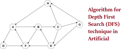
Depth First Search (DFS) technique in Artificial Intelligence

In this article we will discuss about Depth First Search DFS technique in AI , what is searching technique in AI, different types of searches in artificial intelligence like Informed Search, Uninformed search & Depth First Search (DFS) technique in Artificial Intelligence in details with example.

Click her to know details about Depth First Search (DFS) technique in Artificial Intelligence

#Depth First Search (DFS) technique in Artificial Intelligence #artificial intelligence #artificial intelligence edureka artificial intelligence explained #artificial intelligence edureka #artificial intelligence explained #bfs in artificial intelligence #depth first search algorithm in hindi #future of artificial intelligence #state space search in artificial intelligence

0 notes

eccentric-nucleus · 2 years ago

Text

i still really enjoy all of putnam's posts on the df forums exhaustedly explaining that you can't just Optimize The Code.

The way the game is structured is already a nightmare for the cache, which is the actual largest cause of performance issues; just improving cache locality on units a little improved performance by 60%, yet more big ol' structures isn't going to help; moving unit positions out into their own array is likely to be the biggest gain, funnily enough

just saying again over and over that it's not just a matter of precalculating things or using a fancy cool algorithm or w/e else

2 notes · View notes

gaussianray · 3 years ago

Text

Some tips for studying in STEM

So, I'm a TA for an engineering class and I often see a number of similar problems popping up again and again and I thought I'd write down some of those tips to see if they'd help anybody else.

I guess they'd work well enough for most STEM classes too.

In no particular order: 1. Units matter and they can help you a lot When doing anything that you're not quite sure if it's right or not, work out the units and see if they make sense. Some basic rules you should probably be aware: - Derivates (df/dx) have units [function]/[variable] - Integrals have units [function][variable] - You can only add or subtract things with the same units This can help you catch some mistakes regarding unit changes or when you have two similar concepts that have different units (e.g.: capacitance and capacitance per area, both of which are written out as C) 2. Always do a Common Sense Test Does it make sense for a load bearing beam to have a 1 km length (about 0.62 mi)? You have a circuit with a 1 V battery as the sole power source, does it make sense if the current you calculated would dissipate more energy than the UK generates in a year? Sometimes you can get some weird and funky results because you made a mistake somewhere and just stopping to check if the answer makes sense can save you some grief later on. Some common checks you could do: - Is the answer in the expected order of magnitude? - Would this answer waste more energy that's being given to whatever system you're working with? - Does the answer make physical sense in some easy to check special cases? E.g.: If the input is 0, or if the input is infinity or things like that. Some of those checks only really become easy to do after you get some experience but getting used to doing these kind of checks is a useful habit to get into. 3. It's OK to not know something, but know you don't know it in advance As a TA, I try to help people as much as I can and sometimes that includes giving a refresher (or in some cases even teaching) on some things from other subjects. But if you show up the day before the exam or the worksheet deadline and want me to explain the entire subject to you, it's not easy to help you.

Which brings me to another tip ...

4. When asking for help, have actionable questions. If you show up and say "I have no idea how to do this", trying to help you becomes a lot harder because I don't know what I need to say to get you to understand and I won't just tell you the answer or the exact algorithm.

But if you show up saying "I don't understand X" or "Why do we do Y instead of X?" there's a foot in the door to start explaining things and trying to figure out where the foundation is wonky.

Sometimes you can't help it, and that's fine, but try to avoid this if possible. 5. Read carefully and to the end. Sometimes you'll see a problem statement, think "Oh, it's an X question, I know what to do" except it was asking something slightly different. Or was asking you to do X and Y, or was giving you some information that would have made your life a lot easier (or just possible). And even when just studying, most books, tutors or whatnots begin with the "textbook answer" or procedures and will only give the tips and special cases after. If you stop reading as soon as you find something that works you might end up doing more work than necessary. 6. Prose makes all your assignments that much more readable. If you explain your thought process when you're doing something instead of just writing down things you get a few benefits: - You'll have an easier time assimilating the content - Whoever's grading might see you know what you're doing and give you half marks if you messed up the math - If you do make a mistake somewhere and you're trying to figure out where it went wrong, having your thought process written out helps 7. You do the thinking and the computer does the math Using a programming language to do the math avoids a lot of common math problems, mechanical errors (the calculator button was stuck and didn't register) and is easier to debug if anything went wrong. That's all I can think of right now, maybe I'll do a follow up if I remember more stuff and of course, your mileage may vary, these are just things that were useful to me and would help with some of the mistakes I see happening a lot.

#studyblr #study tips #engineering #physics #university

7 notes · View notes

ultragaurav · 5 years ago

Text

Running a k-means Cluster Analysis

K-means algorithm can be summarized as follows:

Specify the number of clusters (K) to be created (by the analyst)

Select randomly k objects from the data set as the initial cluster centers or means

Assigns each observation to their closest centroid, based on the Euclidean distance between the object and the centroid

For each of the k clusters update the cluster centroid by calculating the new mean values of all the data points in the cluster. The centroid of a Kth cluster is a vector of length p containing the means of all variables for the observations in the kth cluster; p is the number of variables.

Iteratively minimize the total within sum of square (Eq. 7). That is, iterate steps 3 and 4 until the cluster assignments stop changing or the maximum number of iterations is reached. By default, the R software uses 10 as the default value for the maximum number of iterations.

Computing k-means clustering in R

We can compute k-means in R with the kmeans function. Here will group the data into two clusters (centers = 2). The kmeans function also has an nstart option that attempts multiple initial configurations and reports on the best one. For example, adding nstart = 25 will generate 25 initial configurations. This approach is often recommended.

k2 <- kmeans(df, centers = 2, nstart = 25) str(k2) ## List of 9 ## $ cluster : Named int [1:50] 1 1 1 2 1 1 2 2 1 1 ... ## ..- attr(*, "names")= chr [1:50] "Alabama" "Alaska" "Arizona" "Arkansas" ... ## $ centers : num [1:2, 1:4] 1.005 -0.67 1.014 -0.676 0.198 ... ## ..- attr(*, "dimnames")=List of 2 ## .. ..$ : chr [1:2] "1" "2" ## .. ..$ : chr [1:4] "Murder" "Assault" "UrbanPop" "Rape" ## $ totss : num 196 ## $ withinss : num [1:2] 46.7 56.1 ## $ tot.withinss: num 103 ## $ betweenss : num 93.1 ## $ size : int [1:2] 20 30 ## $ iter : int 1 ## $ ifault : int 0 ## - attr(*, "class")= chr "kmeans"

The output of kmeans is a list with several bits of information. The most important being:

cluster: A vector of integers (from 1:k) indicating the cluster to which each point is allocated.

centers: A matrix of cluster centers.

totss: The total sum of squares.

withinss: Vector of within-cluster sum of squares, one component per cluster.

tot.withinss: Total within-cluster sum of squares, i.e. sum(withinss).

betweenss: The between-cluster sum of squares, i.e. $totss-tot.withinss$.

size: The number of points in each cluster.

If we print the results we’ll see that our groupings resulted in 2 cluster sizes of 30 and 20. We see the cluster centers (means) for the two groups across the four variables (Murder, Assault, UrbanPop, Rape). We also get the cluster assignment for each observation (i.e. Alabama was assigned to cluster 2, Arkansas was assigned to cluster 1, etc.).

k2 ## K-means clustering with 2 clusters of sizes 20, 30 ## ## Cluster means: ## Murder Assault UrbanPop Rape ## 1 1.004934 1.0138274 0.1975853 0.8469650 ## 2 -0.669956 -0.6758849 -0.1317235 -0.5646433 ## ## Clustering vector: ## Alabama Alaska Arizona Arkansas California ## 1 1 1 2 1 ## Colorado Connecticut Delaware Florida Georgia ## 1 2 2 1 1 ## Hawaii Idaho Illinois Indiana Iowa ## 2 2 1 2 2 ## Kansas Kentucky Louisiana Maine Maryland ## 2 2 1 2 1 ## Massachusetts Michigan Minnesota Mississippi Missouri ## 2 1 2 1 1 ## Montana Nebraska Nevada New Hampshire New Jersey ## 2 2 1 2 2 ## New Mexico New York North Carolina North Dakota Ohio ## 1 1 1 2 2 ## Oklahoma Oregon Pennsylvania Rhode Island South Carolina ## 2 2 2 2 1 ## South Dakota Tennessee Texas Utah Vermont ## 2 1 1 2 2 ## Virginia Washington West Virginia Wisconsin Wyoming ## 2 2 2 2 2 ## ## Within cluster sum of squares by cluster: ## [1] 46.74796 56.11445 ## (between_SS / total_SS = 47.5 %) ## ## Available components: ## ## [1] "cluster" "centers" "totss" "withinss" ## [5] "tot.withinss" "betweenss" "size" "iter" ## [9] "ifault"

We can also view our results by using fviz_cluster. This provides a nice illustration of the clusters. If there are more than two dimensions (variables) fviz_cluster will perform principal component analysis (PCA) and plot the data points according to the first two principal components that explain the majority of the variance.

fviz_cluster(k2, data = df)

Alternatively, you can use standard pairwise scatter plots to illustrate the clusters compared to the original variables.

df %>% as_tibble() %>% mutate(cluster = k2$cluster, state = row.names(USArrests)) %>% ggplot(aes(UrbanPop, Murder, color = factor(cluster), label = state)) + geom_text()

Because the number of clusters (k) must be set before we start the algorithm, it is often advantageous to use several different values of k and examine the differences in the results. We can execute the same process for 3, 4, and 5 clusters, and the results are shown in the figure:

k3 <- kmeans(df, centers = 3, nstart = 25) k4 <- kmeans(df, centers = 4, nstart = 25) k5 <- kmeans(df, centers = 5, nstart = 25) # plots to compare p1 <- fviz_cluster(k2, geom = "point", data = df) + ggtitle("k = 2") p2 <- fviz_cluster(k3, geom = "point", data = df) + ggtitle("k = 3") p3 <- fviz_cluster(k4, geom = "point", data = df) + ggtitle("k = 4") p4 <- fviz_cluster(k5, geom = "point", data = df) + ggtitle("k = 5") library(gridExtra) grid.arrange(p1, p2, p3, p4, nrow = 2)

0 notes

lindarifenews · 6 years ago

Text

Here’s how I used Python to build a regression model using an e-commerce dataset

The programming language of Python is gaining popularity among SEOs for its ease of use to automate daily, routine tasks. It can save time and generate some fancy machine learning to solve more significant problems that can ultimately help your brand and your career. Apart from automations, this article will assist those who want to learn more about data science and how Python can help.

In the example below, I use an e-commerce data set to build a regression model. I also explain how to determine if the model reveals anything statistically significant, as well as how outliers may skew your results.

I use Python 3 and Jupyter Notebooks to generate plots and equations with linear regression on Kaggle data. I checked the correlations and built a basic machine learning model with this dataset. With this setup, I now have an equation to predict my target variable.

Before building my model, I want to step back to offer an easy-to-understand definition of linear regression and why it’s vital to analyzing data.

What is linear regression?

Linear regression is a basic machine learning algorithm that is used for predicting a variable based on its linear relationship between other independent variables. Let’s see a simple linear regression graph:

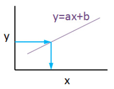
If you know the equation here, you can also know y values against x values. ‘’a’’ is coefficient of ‘’x’’ and also the slope of the line, ‘’b’’ is intercept which means when x = 0, b = y.

My e-commerce dataset

I used this dataset from Kaggle. It is not a very complicated or detailed one but enough to study linear regression concept.

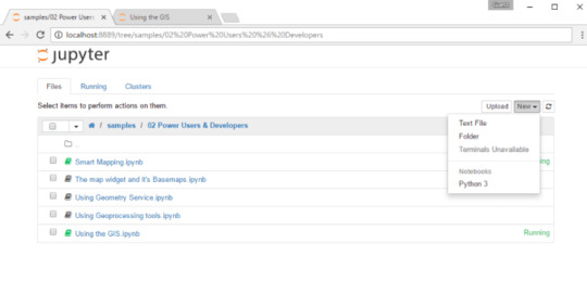
If you are new and didn’t use Jupyter Notebook before, here is a quick tip for you:

Launch the Terminal and write this command: jupyter notebook

Once entered, this command will automatically launch your default web browser with a new notebook. Click New and Python 3.

Now it is time to use some fancy Python codes.

Importing libraries

import matplotlib.pyplot as plt import numpy as np import pandas as pd from sklearn.linear_model import LinearRegression from sklearn.model_selection import train_test_split from sklearn.metrics import mean_absolute_error import statsmodels.api as sm from statsmodels.tools.eval_measures import mse, rmse import seaborn as sns pd.options.display.float_format = '{:.5f}'.format import warnings import math import scipy.stats as stats import scipy from sklearn.preprocessing import scale warnings.filterwarnings('ignore')

Reading data

df = pd.read_csv("Ecom_Customers.csv") df.head()

My target variable will be Yearly Amount Spent and I’ll try to find its relation between other variables. It would be great if I could be able to say that users will spend this much for example, if Time on App is increased 1 minute more. This is the main purpose of the study.

Exploratory data analysis

First let’s check the correlation heatmap:

df_kor = df.corr() plt.figure(figsize=(10,10)) sns.heatmap(df_kor, vmin=-1, vmax=1, cmap="viridis", annot=True, linewidth=0.1)

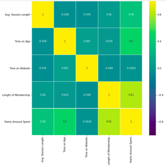
This heatmap shows correlations between each variable by giving them a weight from -1 to +1.

Purples mean negative correlation, yellows mean positive correlation and getting closer to 1 or -1 means you have something meaningful there, analyze it. For example:

Length of Membership has positive and high correlation with Yearly Amount Spent. (81%)

Time on App also has a correlation but not powerful like Length of Membership. (50%)

Let’s see these relations in detailed. My favorite plot is sns.pairplot. Only one line of code and you will see all distributions.

sns.pairplot(df)

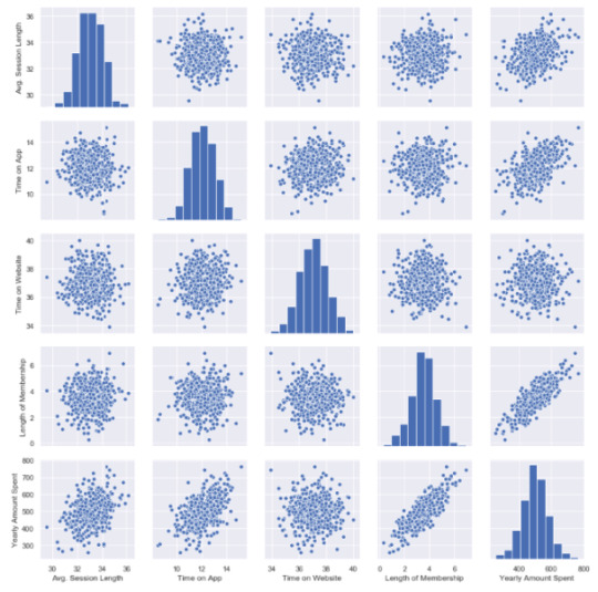
This chart shows all distributions between each variable, draws all graphs for you. In order to understand which data they include, check left and bottom axis names. (If they are the same, you will see a simple distribution bar chart.)

Look at the last line, Yearly Amount Spent (my target on the left axis) graphs against other variables.

Length of Membership has really perfect linearity, it is so obvious that if I can increase the customer loyalty, they will spend more! But how much? Is there any number or coefficient to specify it? Can we predict it? We will figure it out.

Checking missing values

Before building any model, you should check if there are any empty cells in your dataset. It is not possible to keep on with those NaN values because many machine learning algorithms do not support data with them.

This is my code to see missing values:

df.isnull().sum()

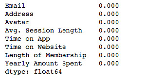
isnull() detects NaN values and sum() counts them.

I have no NaN values which is good. If I had, I should have filled them or dropped them.

For example, to drop all NaN values use this:

df.dropna(inplace=True)

To fill, you can use fillna():

df["Time on App"].fillna(df["Time on App"].mean(), inplace=True)

My suggestion here is to read this great article on how to handle missing values in your dataset. That is another problem to solve and needs different approaches if you have them.

Building a linear regression model

So far, I have explored the dataset in detail and got familiar with it. Now it is time to create the model and see if I can predict Yearly Amount Spent.

Let’s define X and Y. First I will add all other variables to X and analyze the results later.

Y=df["Yearly Amount Spent"] X=df[[ "Length of Membership", "Time on App", "Time on Website", 'Avg. Session Length']]

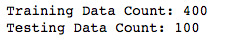
Then I will split my dataset into training and testing data which means I will select 20% of the data randomly and separate it from the training data. (test_size shows the percentage of the test data – 20%) (If you don’t specify the random_state in your code, then every time you run (execute) your code, a new random value is generated and training and test datasets would have different values each time.)

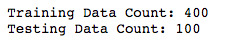
X_train, X_test, y_train, y_test = train_test_split(X, Y, test_size = 0.2, random_state = 465) print('Training Data Count: {}'.format(X_train.shape[0])) print('Testing Data Count: {}'.format(X_test.shape[0]))

Now, let’s build the model:

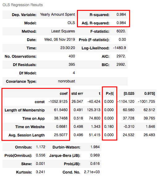
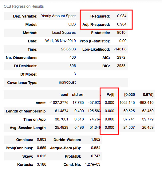
X_train = sm.add_constant(X_train) results = sm.OLS(y_train, X_train).fit() results.summary()

Understanding the outputs of the model: Is this statistically significant?

So what do all those numbers mean actually?

Before continuing, it will be better to explain these basic statistical terms here because I will decide if my model is sufficient or not by looking at those numbers.

What is the p-value?

P-value or probability value shows statistical significance. Let’s say you have a hypothesis that the average CTR of your brand keywords is 70% or more and its p-value is 0.02. This means there is a 2% probability that you would see CTRs of your brand keywords below %70. Is it statistically significant? 0.05 is generally used for max limit (95% confidence level), so if you have p-value smaller than 0.05, yes! It is significant. The smaller the p-value is, the better your results!

Now let’s look at the summary table. My 4 variables have some p-values showing their relations whether significant or insignificant with Yearly Amount Spent. As you can see, Time on Website is statistically insignificant with it because its p-value is 0.180. So it will be better to drop it.

What is R squared and Adjusted R squared?

R square is a simple but powerful metric that shows how much variance is explained by the model. It counts all variables you defined in X and gives a percentage of explanation. It is something like your model capabilities.

Adjusted R squared is also similar to R squared but it counts only statistically significant variables. That is why it is better to look at adjusted R squared all the time.

In my model, 98.4% of the variance can be explained, which is really high.

What is Coef?

They are coefficients of the variables which give us the equation of the model.

So is it over? No! I have Time on Website variable in my model which is statistically insignificant.

Now I will build another model and drop Time on Website variable:

X2=df[["Length of Membership", "Time on App", 'Avg. Session Length']] X2_train, X2_test, y2_train, y2_test = train_test_split(X2, Y, test_size = 0.2, random_state = 465) print('Training Data Count:', X2_train.shape[0]) print('Testing Data Count::', X2_test.shape[0])

X2_train = sm.add_constant(X2_train) results2 = sm.OLS(y2_train, X2_train).fit() results2.summary()

R squared is still good and I have no variable having p-value higher than 0.05.

Let’s look at the model chart here:

X2_test = sm.add_constant(X2_test) y2_preds = results2.predict(X2_test) plt.figure(dpi = 75) plt.scatter(y2_test, y2_preds) plt.plot(y2_test, y2_test, color="red") plt.xlabel("Actual Scores", fontdict=ex_font) plt.ylabel("Estimated Scores", fontdict=ex_font) plt.title("Model: Actual vs Estimated Scores", fontdict=header_font) plt.show()

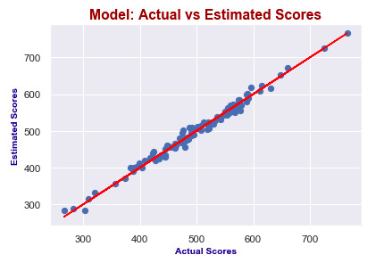
It seems like I predict values really good! Actual scores and predicted scores have almost perfect linearity.

Finally, I will check the errors.

Errors

When building models, comparing them and deciding which one is better is a crucial step. You should test lots of things and then analyze summaries. Drop some variables, sum or multiply them and again test. After completing the series of analysis, you will check p-values, errors and R squared. The best model will have:

P-values smaller than 0.05

Smaller errors

Higher adjusted R squared

Let’s look at errors now:

print("Mean Absolute Error (MAE) : {}".format(mean_absolute_error(y2_test, y2_preds))) print("Mean Squared Error (MSE) : {}".format(mse(y2_test, y2_preds))) print("Root Mean Squared Error (RMSE) : {}".format(rmse(y2_test, y2_preds))) print("Root Mean Squared Error (RMSE) : {}".format(rmse(y2_test, y2_preds))) print("Mean Absolute Perc. Error (MAPE) : {}".format(np.mean(np.abs((y2_test - y2_preds) / y2_test)) * 100))

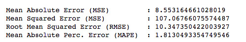
If you want to know what MSE, RMSE or MAPE is, you can read this article.

They are all different calculations of errors and now, we will just focus on smaller ones while comparing different models.

So, in order to compare my model with another one, I will create one more model including Length of Membership and Time on App only.

X3=df[['Length of Membership', 'Time on App']] Y = df['Yearly Amount Spent'] X3_train, X3_test, y3_train, y3_test = train_test_split(X3, Y, test_size = 0.2, random_state = 465) X3_train = sm.add_constant(X3_train) results3 = sm.OLS(y3_train, X3_train).fit() results3.summary()

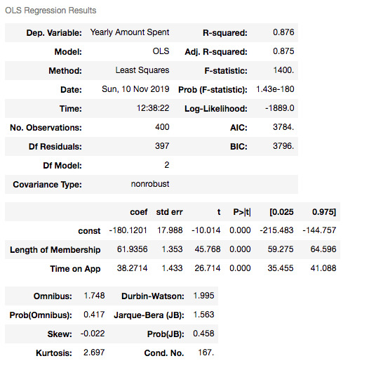
X3_test = sm.add_constant(X3_test) y3_preds = results3.predict(X3_test) plt.figure(dpi = 75) plt.scatter(y3_test, y3_preds) plt.plot(y3_test, y3_test, color="red") plt.xlabel("Actual Scores", fontdict=eksen_font) plt.ylabel("Estimated Scores", fontdict=eksen_font) plt.title("Model Actual Scores vs Estimated Scores", fontdict=baslik_font) plt.show() print("Mean Absolute Error (MAE) : {}".format(mean_absolute_error(y3_test, y3_preds))) print("Mean Squared Error (MSE) : {}".format(mse(y3_test, y3_preds))) print("Root Mean Squared Error (RMSE) : {}".format(rmse(y3_test, y3_preds))) print("Mean Absolute Perc. Error (MAPE) : {}".format(np.mean(np.abs((y3_test - y3_preds) / y3_test)) * 100))

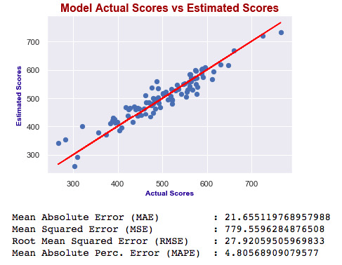
Which one is best?

As you can see, errors of the last model are higher than the first one. Also adjusted R squared is decreased. If errors were smaller, then we would say the last one is better – independent of R squared. Ultimately, we choose smaller errors and higher R squared. I’ve just added this second one to show you how you can compare the models and decide which one is the best.

Now our model is this:

Yearly Amount Spent = -1027.28 + 61.49x(Length of Membership) + 38.76x(Time on App) + 25.48x(Avg. Session Length)

This means, for example, if we can increase the length of membership 1 year more and holding all other features fixed, one person will spend 61.49 dollars more!

Advanced tips: Outliers and nonlinearity

When you are dealing with the real data, generally things are not that easy. To find linearity or more accurate models, you may need to do something else. For example, if your model isn’t accurate enough, check for outliers. Sometimes outliers can mislead your results!

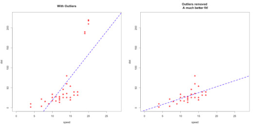
Source: http://r-statistics.co/Outlier-Treatment-With-R.html

Apart from this, sometimes you will get curved lines instead of linear but you will see that there is also a relation between variables!

Then you should think of transforming your variables by using logarithms or square.

Here is a trick for you to decide which one to use:

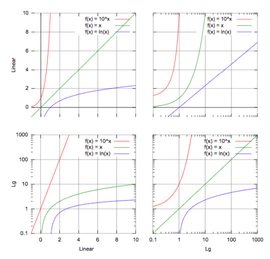
Source: https://courses.lumenlearning.com/boundless-algebra/chapter/graphs-of-exponential-and-logarithmic-functions/

For example, in the third graph, if you have a line similar to the green one, you should consider using logarithms in order to make it linear!

There are lots of things to do so testing all of them is really important.

Conclusion

If you like to play with numbers and advance your data science skill set, learn Python. It is not a very difficult programming language to learn, and the statistics you can generate with it can make a huge difference in your daily work.

Google Analytics, Google Ads, Search Console… Using these tools already offers tons of data, and if you know the concepts of handling data accurately, you will get very valuable insights from them. You can create more accurate traffic forecasts, or analyze Analytics data such as bounce rate, time on page and their relations with the conversion rate. At the end of the day, it might be possible to predict the future of your brand. But these are only a few examples.

If you want to go further in linear regression, check my Google Page Speed Insights OLS model. I’ve built my own dataset and tried to predict the calculation based on speed metrics such as FCP (First Contentful Paint), FMP (First Meaningful Paint) and TTI (Time to Interactive).

In closing, blend your data, try to find correlations and predict your target. Hamlet Batista has a great article about practical data blending. I strongly recommend it before building any regression model.

The post Here’s how I used Python to build a regression model using an e-commerce dataset appeared first on Search Engine Land.

Here’s how I used Python to build a regression model using an e-commerce dataset published first on https://likesfollowersclub.tumblr.com/

0 notes