#iferror(sum(iferror(vlookup

[zirrah-writes]

me writing a formula nested in a formula nested in a formula like a set of russian dolls and spending five minutes counting the parentheses

* (Oh, these parentheses I keep opening?

* (I'm collecting them.

* (Right now, I'm 1,762 parentheses deep.

* (Oh, my precious parentheses... (I don't ever want to close them!

[graysongarelick]

Mastering Excel: Grayson Garelick Shares Essential Tips and Tricks for Beginners

In today's data-driven world, proficiency in Microsoft Excel is a valuable skill that can open doors to countless opportunities in various industries. Whether you're a student, a professional, or an entrepreneur, mastering Excel can significantly enhance your productivity, efficiency, and decision-making capabilities. To help beginners embark on their journey to Excel mastery, seasoned Excel expert Grayson Garelick shares some essential tips and tricks that lay the foundation for success.

Get Comfortable with the Basics: Before diving into advanced features, it's crucial to familiarize yourself with the basics of Excel. Learn how to navigate the interface, enter data, and perform simple calculations using formulas like SUM, AVERAGE, and COUNT. Understanding these foundational concepts will set you up for success as you progress to more complex tasks.

Explore Keyboard Shortcuts: Excel offers a plethora of keyboard shortcuts that can save you time and streamline your workflow. Take the time to learn commonly used shortcuts for tasks like copying and pasting, formatting cells, and navigating between worksheets. Memorizing these shortcuts will make you more efficient and productive in Excel.

Practice Regularly: Like any skill, proficiency in Excel comes with practice. Dedicate time each day to practice using Excel and experimenting with different features and functions. The more you practice, the more comfortable and confident you'll become in navigating Excel and performing various tasks.

Utilize Online Resources: Take advantage of the wealth of online resources available to learn Excel. Websites like Microsoft's official Excel help center, YouTube tutorials, and online courses offer valuable insights and guidance for beginners. Additionally, forums and communities like Stack Overflow and Reddit can be excellent places to ask questions and seek advice from experienced Excel users.

Master Essential Formulas and Functions: Formulas and functions are the backbone of Excel's functionality, allowing you to perform calculations, manipulate data, and analyze trends. Start by mastering essential formulas like VLOOKUP, SUMIF, and IFERROR, which are commonly used in data analysis and reporting. As you become more comfortable with these formulas, you can explore more advanced functions to expand your skill set further.

Learn Data Visualization Techniques: Excel offers powerful tools for visualizing data, such as charts, graphs, and pivot tables. Learning how to create visually compelling and informative visualizations can help you communicate insights effectively and make informed decisions based on your data. Experiment with different chart types and formatting options to find the best visualization for your data.

Stay Organized: Keeping your Excel workbooks organized is essential for efficiency and productivity. Use descriptive file names and folder structures to easily locate and access your files. Within your workbooks, use clear and consistent naming conventions for sheets, ranges, and cells. Additionally, consider using color coding and formatting techniques to visually distinguish different types of data.

Stay Updated: Excel is continuously evolving, with new features and updates released regularly. Stay informed about the latest developments by subscribing to Excel-related blogs, newsletters, and forums. Keeping up-to-date with the latest features and best practices will ensure that you're maximizing Excel's potential and staying ahead of the curve.

By following these tips and tricks shared by Excel expert Grayson Garelick, beginners can lay a solid foundation for mastering Excel and unlocking its full potential. With dedication, practice, and a willingness to learn, anyone can become proficient in Excel and leverage its powerful capabilities to excel in their personal and professional endeavors.

[gvtacademy]

Unlock Advanced Excel Secrets with GVT Academy

Excel stands out as an incredibly versatile tool for organizing, analyzing, and visualizing data. Whether you are working in finance, marketing, or data analysis, mastering Excel can significantly boost your productivity and decision-making capabilities. At GVT Academy, we offer top-notch Advanced Excel training in Noida, empowering professionals to unlock Excel’s full potential. In this article, we’ll share some of the advanced Excel secrets that every professional should know, whether you're an Excel novice or a seasoned user looking to refine your skills.

1. Mastering Pivot Tables for Data Analysis

Pivot Tables stand out as one of Excel's most versatile and impactful tools for data analysis. This tool allows you to summarize large datasets quickly, enabling you to analyze and report data efficiently. Advanced Excel training in Noida can teach you how to create dynamic Pivot Tables that allow for deeper insights. With Pivot Tables, you can group data, calculate averages, totals, and percentages, and filter the data in multiple ways. This is essential for anyone working with large datasets and reporting requirements.

2. Advanced Functions and Formulas

Excel is packed with a variety of functions and formulas that can simplify complex calculations. While SUM and AVERAGE are often the go-to functions, Excel has advanced formulas such as INDEX & MATCH, IFERROR, VLOOKUP, and XLOOKUP. These can be used to perform data lookups, error handling, and complex conditional logic in your spreadsheets.

At GVT Academy, we dive deeper into Advanced Excel training to help you understand how to combine functions for more complex operations. Learning how to use these functions together will enable you to automate calculations and reduce errors, saving time and effort in the process.

3. Power Query for Data Importing and Transformation

Power Query in Excel enables users to link, import, and organize data from multiple sources efficiently. With Power Query, you can automatically refresh data and perform advanced data transformations like filtering, merging, and splitting columns. Whether you’re working with large databases or external data sources, Power Query simplifies these tasks and makes the process much more efficient.

If you’re new to Power Query, Advanced Excel training in Noida at GVT Academy can provide you with hands-on experience in setting up Power Query to transform raw data into a format that’s ready for analysis.

4. Data Validation and Conditional Formatting

Data validation ensures that the data entered into your Excel sheet meets specific criteria, preventing errors. With this feature, you can restrict values to specific ranges, create drop-down lists, and even set custom validation rules. Additionally, conditional formatting lets you highlight specific cells based on certain conditions, such as cells that are greater than a particular value or cells with duplicate entries.

Learning how to use these tools effectively will ensure that your data remains accurate and easy to read, and will help prevent mistakes when inputting or analyzing data.

5. Macros and VBA Programming

If you regularly perform repetitive tasks, learning how to record macros or write VBA (Visual Basic for Applications) code can save you hours. Macros automate tasks like formatting, calculations, and report generation with a single click. VBA programming takes it a step further by allowing you to create custom functions and more complex automation.

At GVT Academy, we offer specialized training on how to harness the power of macros and VBA, giving you the skills to automate almost any process in Excel. This is particularly beneficial for professionals looking to improve workflow efficiency.

6. Advanced Charting Techniques

While Excel offers basic charts like bar and line graphs, its advanced charting capabilities are often underutilized. Learning to create dynamic charts, such as sparklines, heat maps, and waterfall charts, can significantly enhance your ability to present complex data visually. Customizing chart axes, formatting, and adding trendlines can make your data visualization more impactful.

GVT Academy’s Advanced Excel training covers these techniques in detail, allowing professionals to master the art of visual storytelling through data.

7. Excel for Business Intelligence

Excel is also a powerful tool for business intelligence when combined with tools like Power Pivot and Power BI. Power Pivot allows you to analyze massive datasets by creating relationships between tables, and Power BI extends these capabilities with interactive dashboards and reporting.

For professionals looking to dive into business intelligence, Excel and Advanced Excel training in Noida at GVT Academy offers practical guidance on integrating these tools with Excel, giving you a competitive edge in the workplace.

Conclusion

Excel goes far beyond being just a basic spreadsheet application. With the right training, it can become your go-to solution for data analysis, reporting, and business intelligence. GVT Academy’s Advanced Excel training in Noida equips professionals with the skills they need to excel in today’s data-driven world. By mastering these advanced features, you’ll enhance your productivity, reduce errors, and make better, data-backed decisions.

Elevate your Excel expertise by enrolling in GVT Academy’s Advanced Excel training in Noida and discover its true potential!

[makemonewithchatgpt]

100 chatgpt command prompts for mastering in Microsoft excel

Elevate your Microsoft Excel mastery with the power of ChatGPT command prompts. Discover the best ChatGPT prompts tailored for optimizing your Microsoft Excel experience. Unleash the potential of this dynamic combination to streamline tasks and achieve unparalleled efficiency in your spreadsheet workflows.

Whether you’re a novice or seasoned user, harness the capabilities of ChatGPT to enhance your Excel skills and achieve exceptional results.

1.”Generate a formula to sum the values in column A.”

2.”Create a VLOOKUP formula to retrieve data from another sheet.”

3.”Explain the difference between SUM and SUMIF functions in Excel.”

4.”Generate a bar chart for the data in cells A1 to B10.”

5.”How do I merge cells in Excel and center the text?”

6.”Write a formula to calculate the average of a range of cells.”

7.”Create a macro to automate a repetitive task in Excel.”

8.”How can I protect a specific range of cells with a password?”

9.”Sort data in descending order based on values in column C.”

10″Generate a pivot table summarizing sales data by month.”

11.”What is the purpose of the IFERROR function in Excel?”12.”How do I freeze panes to keep row and column headers visible?”

Code: yFVOQjwb 13.”Create a conditional formatting rule for cells containing errors.”

14.”Generate a random sample of data using the RAND function.”

15.”Explain the steps to create a drop-down list in Excel.”

16.”Write a formula to concatenate text in cells A1 and B1.”

17.”How can I find and replace specific text in a worksheet?”

18.”Create a line chart to visualize the trend in sales data.”

19.”What is the purpose of the INDEX and MATCH functions in Excel?”

20.”How do I transpose data from rows to columns in Excel?”

100 chatgpt command prompts for mastering in Microsoft excel

[allenbalif]

Formulas and Functions

Formulas and functions are essential elements in various applications, especially in spreadsheet software like Microsoft Excel or Google Sheets. They help perform calculations, manipulate data, and automate tasks. Here are some common formulas and functions:

Basic Arithmetic Formulas:

Addition:

=A1 + B1

Subtraction:

=A1 - B1

Multiplication:

=A1 * B1

Division:

=A1 / B1

Common Functions:

SUM: Adds up a range of cells.

=SUM(A1:A10)

AVERAGE: Calculates the average of a range of cells.

=AVERAGE(A1:A10)

MAX: Returns the maximum value in a range of cells.

=MAX(A1:A10)

MIN: Returns the minimum value in a range of cells.

=MIN(A1:A10)

IF: Performs conditional logic.

=IF(A1>B1, "Yes", "No")

VLOOKUP: Searches for a value in the first column of a table and returns a value in the same row from another column.

=VLOOKUP(A1, B1:C10, 2, FALSE)

HLOOKUP: Similar to VLOOKUP but searches for a value in the first row of a table.

=HLOOKUP(A1, B1:C10, 2, FALSE)

INDEX/MATCH: An alternative to VLOOKUP or HLOOKUP for more flexible lookups.

=INDEX(C1:C10, MATCH(A1, B1:B10, 0))

CONCATENATE (or CONCAT in Excel 2016 and later): Combines two or more strings of text.

=CONCATENATE(A1, " ", B1)

IFERROR: Handles errors by specifying an alternative value or action. excel =IFERROR(A1/B1, "Error in calculation")

These are just a few examples, and the functionalities may vary slightly between spreadsheet applications. Understanding these formulas and functions can significantly enhance your ability to manipulate and analyze data in spreadsheets.

Watch Now:- The Knowledge Academy

[esytes-encyclopedia]

The Excel Formulas You Need to Know to Save Time

There are numerous Excel formulas that can be useful in various situations, but here are some essential Excel formulas that most users should know: SUM: Adds up all the numbers in a range of cells. Example: =SUM(A1:A5). AVERAGE: Calculates the average of a range of numbers. Example: =AVERAGE(B1:B10). MAX: Returns the largest number in a range. Example: =MAX(C1:C20). MIN: Returns the smallest number in a range. Example: =MIN(D1:D15). COUNT: Counts the number of cells that contain numbers in a range. Example: =COUNT(E1:E30). IF: Performs a conditional operation. It returns one value if a condition is true and another if it's false. Example: =IF(A1>10, "Yes", "No"). VLOOKUP: Searches for a value in the first column of a table and returns a value in the same row from a specified column. Example: =VLOOKUP(G1, A1:B10, 2, FALSE). HLOOKUP: Similar to VLOOKUP, but searches horizontally in a table. Example: =HLOOKUP(G1, A1:G10, 3, FALSE). INDEX and MATCH: Used together, these functions can perform powerful lookups. INDEX returns a value from a specific row and column in a range, and MATCH searches for a value in a range and returns its relative position. Example: =INDEX(A1:B10, MATCH(G1, A1:A10, 0), 2). CONCATENATE (or CONCAT): Combines text from multiple cells into one cell. Example: =CONCATENATE(A1, " ", B1). LEFT and RIGHT: Extracts a specified number of characters from the left or right of a cell's content. Example: =LEFT(A1, 3). LEN: Returns the length (number of characters) of a text string. Example: =LEN(A1). TRIM: Removes extra spaces from text. Example: =TRIM(A1). DATE: Creates a date value. Example: =DATE(2023, 9, 7). TODAY: Returns the current date. Example: =TODAY(). NOW: Returns the current date and time. Example: =NOW(). SUMIF: Adds up all numbers in a range that meet a specified condition. Example: =SUMIF(B1:B10, ">50"). COUNTIF: Counts the number of cells in a range that meet a specified condition. Example: =COUNTIF(C1:C20, "=75"). IFERROR: Returns a custom value if a formula generates an error. Example: =IFERROR(A1/B1, "N/A"). SUMIFS: Adds up numbers in a range that meet multiple conditions. Example: =SUMIFS(B1:B10, A1:A10, "Apples", C1:C10, ">10"). COUNTIFS: Counts the number of cells that meet multiple criteria. Example: =COUNTIFS(A1:A10, "Bananas", B1:B10, ">5"). AVERAGEIFS: Calculates the average of a range based on multiple criteria. Example: =AVERAGEIFS(D1:D15, E1:E15, "Red", F1:F15, ">50"). IF, AND, OR: Combining these functions can create more complex conditional statements. Example: =IF(AND(A1>10, B1="Yes"), "Pass", "Fail"). SUMPRODUCT: Multiplies corresponding components in arrays and returns the sum of those products. Example: =SUMPRODUCT(A1:A5, B1:B5). TEXT: Converts a number into text with a specified format. Example: =TEXT(NOW(), "dd-mmm-yyyy hh:mm:ss"). PROPER: Capitalizes the first letter of each word in a text string. Example: =PROPER("john doe"). UPPER and LOWER: Converts text to all uppercase or all lowercase. Example: =UPPER("hello") and =LOWER("WORLD"). SUBTOTAL: Performs various aggregate functions (e.g., SUM, AVERAGE) on filtered data sets. Example: =SUBTOTAL(109, B1:B100). RANK: Returns the rank of a number within a list. Example: =RANK(A1, A1:A10, 1). ROUND: Rounds a number to a specified number of decimal places. Example: =ROUND(A1, 2). ROUNDUP and ROUNDDOWN: Round a number up or down to the nearest specified decimal place. Example: =ROUNDUP(A1, 0) and =ROUNDDOWN(B1, 1). PI: Returns the mathematical constant Pi (π). Example: =PI(). RAND and RANDBETWEEN: Generates random numbers. RAND() returns a decimal between 0 and 1, while RANDBETWEEN(min, max) generates a random integer within a specified range. DAYS: Calculates the number of days between two dates. Example: =DAYS(B1, C1). NETWORKDAYS: Calculates the number of working days between two dates, excluding weekends and specified holidays. Example: =NETWORKDAYS(B1, C1, holidays). DGET: Retrieves a single value from a database based on specified criteria. PMT: Calculates the monthly payment for a loan based on interest rate, principal, and term. Example: =PMT(0.05/12, 5*12, 10000). NPV: Calculates the net present value of a series of cash flows based on a discount rate. Example: =NPV(0.1, C1:C5). IRR: Calculates the internal rate of return for a series of cash flows. Example: =IRR(D1:D5). Conclusion: In conclusion, Excel offers a rich arsenal of formulas and functions that cater to a wide range of data manipulation and analysis needs. The formulas and functions listed in the previous responses cover the fundamentals, from basic arithmetic calculations to conditional statements, text manipulation, and advanced financial and statistical analysis. Familiarity with these Excel formulas empowers users to efficiently manage data, perform calculations, and derive valuable insights. Read the full article

[makecareersolution]

15 Advanced Excel Formulas You Must Know

Introduction

Microsoft Excel is a powerful tool for data analysis and management. It is used by businesses and individuals worldwide to organize and analyze data, create charts and graphs, and automate tasks. Excel offers a wide range of built-in functions, but advanced Excel formulas take your skills to the next level.

VLOOKUP

VLOOKUP is one of the most commonly used Excel formulas. It is used to find and retrieve data from a specific column in a table. It works by matching a lookup value to a corresponding value in the first column of a table and returning a value in the same row from a specified column.

INDEX-MATCH

INDEX-MATCH is an alternative to VLOOKUP. It is used to find and retrieve data from a specific row or column in a table. It works by matching a lookup value to a corresponding value in a specified column or row and returning a value from a specified row or column.

SUMIFS

SUMIFS is used to sum values in a range that meet multiple criteria. It works by specifying the range to sum, as well as the criteria to be met for each corresponding cell in a separate range.

COUNTIFS

COUNTIFS is used to count the number of cells in a range that meet multiple criteria. It works by specifying the range to count, as well as the criteria to be met for each corresponding cell in a separate range.

IFERROR

IFERROR is used to replace an error value with a specific value or message. It works by testing a formula for an error value and returning a specified value if an error is detected.

CONCATENATE

CONCATENATE

 is used to join two or more text strings into a single string. It works by specifying the text strings to be joined and the separator to be used between them.

LEFT, RIGHT, and MID

LEFT, RIGHT, and MID are used to extract a specific number of characters from a text string. LEFT is used to extract characters from the beginning of a string, RIGHT is used to extract characters from the end of a string, and MID is used to extract characters from the middle of a string.

LEN

LEN is used to determine the length of a text string. It works by counting the number of characters in a string.

TRIM

TRIM is used to remove extra spaces from a text string. It works by removing all leading and trailing spaces, as well as any extra spaces between words.

SUBSTITUTE

SUBSTITUTE is used to replace a specific text string within a larger text string with a different text string. It works by specifying the text string to be replaced, the text string to replace it with, and the text string in which the replacement is to occur.

NETWORKDAYS

NETWORKDAYS is used to calculate the number of working days between two dates. It works by excluding weekends and specified holidays from the calculation.

EOMONTH

EOMONTH is used to calculate the last day of the month based on a specified date. It works by adding a specified

If you are looking to enhance your Excel skills, then learning advanced Excel formulas is the next step for you. Knowing advanced Excel formulas will help you automate complex calculations, save time, and improve your overall productivity. In this Blog, we have discussed 15 advanced Excel formulas that you must know.

[hiyoko-channnel]

Excelで5種類の便利なカレンダー作成！関数のみからVBAまで難易度別！【解説】

動画を見ながら実践できるようにコンテンツを配布中 ▼カレンダー①年月を入力するだけで自動作成！▼ ▼カレンダー②年月を入力するだけで自動作成！▼ ▼カレンダー③予定の有無が一目で分かる！▼ ▼カレンダー④シート自動生成システムを作成▼ ▼カレンダー⑤一瞬で作成する自作アドイン▼ 【おすすめの参考書】 +—————————+ ■IT予備メンバー募集 +—————————+ 勉強を継続するためのサポートを行います。 その中には、動画内の作品の配布や質問し放題などを用意しています。 ▼詳しくはこちら▼ +—————————+ ■目次 +—————————+ 00:00　カレンダー①【難易度：★★】 00:13　カレンダー②【難易度：★】 25:11　カレンダー③【難易度：★★】 38:26　カレンダー④(VBAあり)【難易度：★★☆】 1:02:57　カレンダー⑤(VBAあり)【難易度：★★★…

[makeover-blog1]

Learn MS Excel Formulas and Functions. Create Basic and Advanced Excel Formulas….

Learn MS Excel Formulas and Functions. Create Basic and Advanced Excel Formulas. Make an Excel Template Project. What you’ll learn Learn Excel Formulas and Functions from Zero. Learn how to build a professional level Excel Template using Excel functions. Requirements Microsoft Office Software Installed. Description Teaching11Courses on Excel and Data Analysis! OVER25000 visitors visit my blog ExcelDemy dotcom every month!! OVER 15000successful students have already takenmy online courses since November 2015with375totalReviews!!! Course Updated:Nov 01.2016 Excel formulas and functions are the heart of Microsoft Excel spreadsheet. They are essential to manipulating data and obtaining useful information from your Excel workbooks. Without Excel formulas and functions Excel spreadsheet would simply be a fancy word-processing document. Welcome to my Excel Formulas and Functions course. Lets discuss now what you will learn from this course. Operators and Precedence of Operators: I will start from zero and if you dont know about the operators and precedence of operators that Excel uses in its formulas then it will be tough for you to decode complex Excel formulas. So I have covered them in very details. How to use built-in Excel functions: Then you will learn how to use built-in excel functions into the Excel formulas using the Insert Function and Function Arguments dialog box. Subtotal Function: You will find many uses of Subtotal function if you are using Excel with your finance related jobs. So this function is covered in details at the start of the course. Relative Absolute and Mixed Cell References: You will work with these three concepts time to time when you will build excel formulas. So they have got a good time in the course. Formulas with Tables: Understanding how formulas work with Excel tables is very important. I have used two lectures to cover Excel formulas with tables. In the second lecture structured referencing with Excel tables has been discussed. Then you will learn how to handle circular references with Excel formulas how named cells and ranges work with Excel formulas and so on. Mathematical functions are very important in your daily work with finance or any kind of jobs. In this course you will learn about SUM AVERAGE MAX MIN INT MOD ROUND RAND and RANDBETWEEN Excel functions. Counting related excel functions are also covered in this course. Then you will work with 3-D Referencing with Excel Formulas. In Advanced Excel formulas you will learn: IF IFERROR DATE related functions Text manipulating functions and many more. Manipulating Text using Excel Functions: There is a section where you will learn how to manipulate text using Excel formulas and functions. Then you have worked with VLOOKUP INDEX and Array formulas. And at the end of the course you will build a professional Excel template where you will learn how to make complex Excel formulas using Excel functions. Here is not the end of the course. Time to time I shall add more lectures to the course that will teach you how to face real life problems using Excel formulas and functions. =====> CLICK HERE TO ENROLL FOR FREE <=====

The post Learn MS Excel Formulas and Functions. Create Basic and Advanced Excel Formulas…. appeared first on Good Info.

[spainjust]

Compare two columns in excel and return differences

#Compare two columns in excel and return differences how to#

#Compare two columns in excel and return differences windows#

Please state your queries regarding Conditional formatting down in the comment box. Please do check out other articles on Conditional Formatting. You can compare two columns in excel for differences using Conditional Formatting in Excel. You can customize your highlight Index and formatting for your data by clicking on the Custom Format option as shown below. You can find duplicate values are highlighted with Green fill with Dark Green Text as shown below. Select the Duplicate option from the dropdown list as shown in above snapshot. Select the cells you need to apply conditional formatting.��lick Home > Conditional Formatting > Highlight Cell Rules > Duplicate values So for this, we are going to use Conditional formatting. Instead of having the TRUE or FALSE values, you can set the value for matching or different data. This is similar to the above method, but it comes with the advantage that you can customize the displayed value. We need to find out the repeated or duplicate names. A different method to analyze Excel data from two columns is to use an IF function. Here we have a list of names in all three columns.

#Compare two columns in excel and return differences how to#

Let’s understand how to compare two columns in excel taking the below example. For this, we will create a rule in Conditional Formatting. It allows you to apply formatting basis on the cell values such as colours, icons and data bars. Conditional Formatting provides a way to visualize data and make worksheets easier to understand. It would be difficult to see various trends just for examining your Excel worksheet. You can do this using the UNIQUE function, which is available in Excel 365 or Excel Online.In this article, we will compare two columns using the Conditional Formatting tool in Excel 2016. It would also be great to exclude empty cells in the array. To get rid of #N/A, let’s nest our VLOOKUP formula with IFERROR as follows: =IFERROR(VLOOKUP(A2:A66,C2:C66,1,FALSE),"")

1 – the column to return the matching values from.

#Compare two columns in excel and return differences windows#

Select an array, which will be not less than the arrays in your VLOOKUP formula, insert the following formula to the formula bar and press Ctrl+Shift+Enter for Windows ( Command+Return for Mac) – this will apply an array formula in Excel: =VLOOKUP(A2:A66,C2:C66,1,FALSE) We can do this using the VLOOKUP function applied as an array formula. As a result, the ISERROR function returns FALSE and the IF function. Explanation: the MATCH function in cell C1 returns the number 5 (letter A found at position 5 in the range B1:B7). Display the duplicates in the first column (these values also occur in the second column). What we need is to compare the values from these columns to identify duplicates – values that are present in both columns. Let's start by comparing two columns and displaying the duplicates. On the dataset, we have two columns: Old users and New users. Read more about Microsoft Excel integrations for data export on a schedule. Excel, for example, uses a different file for each worksheet. We imported a dataset from Google Sheets to Excel using Coupler.io, a solution for automatic data exports from multiple apps and sources. This will look at the JANEXP file, find the range ITEMTOTS, and return the sum of the. The VLOOKUP function will help you complete this task. Let’s say you have two columns with some textual or numeric values and you need to identify which values are present in both columns and which aren’t.

[globalteachonline]

What you'll learn Learn functions & formulas with the easiest & the most comprehensible examples.Learn to prepare for the most Excel practical examinations.Learn to master usage of Excel in an office environment.Learn various charts & Pivot Table with the easiest examples.Learn practically MS Excel from basic to advance.Learn unique & difficult combination of different functions in Excel.Students who want to learn Excel. Professionals who want to improve in Excel & bring more clarity to various options.This course contains the basics to advance the learning of Excel. The quick explanation technique in video saves a lot of time, it has various functions & formulas explained in the easiest, most accurate & most comprehensible examples for all. This course explains what are rows & columns how to hide/unhide & delete them, cell & range of cells & how to drag cells, how many spreadsheets in one Excel workbook, different Tabs & Ribbons, what is the Quick Access Toolbar, Name Box & Formula Bar, how to navigate Excel & how to save & save As. The application of BODMAS in Excel, learn when it will be applicable & when not. In this course, you will get to learn the basics & advanced usage of functions like LEFT, RIGHT, MID, CONCATENATE, NOW, TODAY, EOMONTH, NETWORKDAYS, NETWORKDAYSINTL, WORKDAY, SUBTOTAL, MOD & QUOTIENT, IFERROR, List of Errors & Various Error Alerts, LOOKUP, HLOOKUP, HLOOKUP, SUMPRODUCT, SUM(Array)VLOOKUP, PMT, PPMT, IPMT, FV, NPV & IRR, XNPV & XIRR, SUM, AVERAGE, MIN, MAX, COUNT, IF, IF AND, IF OR, IF NOT, NESTED IF, INDEX & MATCH with Vlookup, MAX, Array (Ctrl + Shift + Enter) & many more with a combination of two or more functions. This course will explain variously charts available in Excel, it also explains the distinction between normal table/chart & Pivot table/chart. The explanation of various shortcuts available in Excel will speed up our day to day work. I am looking forward to you, subscribing to the course.Who this course is for:This course is designed for the beginner, intermediate & advanced users of Excel.This course is best for students wanting to practically learn Excel.This course is best for professionals wanting to bring more clarity in Excel & learn new methods.This course can help various business owners & employees to get hands-on Excel.Beginner

[concordeducations]

3-Hour Excel Automation Boot Camp: Top Ten Excel Functions, Lookup Functions (VLOOKUP, HLOOKUP, MATCH, INDEX) Basics of Excel Macros with an Introduction to VBA

Excel functions can greatly enhance your ability to perform tasks in day to day activities in Excel. While there are hundreds of functions available, there are 10 functions that all Excel users should know. Whether you are an office worker, or a small business owner using Excel to keep track of your finances or just the casual user, these Excel functions can be very important time savers and enhance your ability to create better performing spreadsheets!

Learning about the lookup functions in Excel will allow you to match data between databases. VLOOKUP enables you to quickly and easily look for a value down a column of data and return a value from the same row in a different column. Perfect for when working with large tabular data. INDEX and MATCH work in a similar way but provide more flexibility.

Why Should You Attend

As an intermediate to advanced level user of Excel, not only do you want to take your knowledge and skills to the next level, you want to produce meaningful, impactful and insightful reports in the shortest time possible. These features of the application will help you to do just that.

Objectives of the Presentation 

This Microsoft Excel training session covers THREE intermediate to advanced features of Excel that provide automation within the application.

Formulas are equations that can perform calculations, return information, manipulate the contents of other cells, test conditions, and more. Explore what are considered the top 10 functions.

Lookup functions in Excel are far superior to manually searching for specific data elements in a spreadsheet. VLOOKUP, HLOOKUP, INDEX and MATCH are some of the most well-known (and most useful) functions in Excel.

Being able to create and edit macros is one of the must have skills for Excel Power Users. Having this knowledge will save you hours of time by allowing you to automate any Excel-based task or process. If you’ve never create macros or used VBA before, this advanced Excel training is for you.

Areas Covered in the Session  » Learn many statistical functions including SUM, AVERAGE, MAX, MIN and COUNT  » Use IF and its counterparts COUNTIF, SUMIF, and AVERAGEIF  » Calculate dates using TODAY, NOW  » Learn many functions to manipulate text once imported including LEFT, RIGHT, LEN, TRIM and CONCATENATE  » Learn the arguments in the VLOOKUP function  » Understand the importance of absolute references within many lookup functions  » Use VLOOKUP to perform approximate matches  » Simplify multiple-field look-ups with concatenation (combining fields into a single cell)  » Use VLOOKUP to look up data from another workbook  » Learn how VLOOKUP stops looking after it finds an initial match within a list  » Explore why VLOOKUP sometimes returns #N/A instead of a desired result  » Learn about the IFNA function available in Excel 2013 and later  » Use the IFERROR function to display something other than an #N/A error value when VLOOKUP can’t find a match  » See how the HLOOKUP function enables you to perform horizontal matches  » Learn why the INDEX and MATCH combination often is superior to VLOOKUP or HLOOKUP  » Use the MATCH function to find the position of an item on a list  » Learn the difference between workbook macros and personal macros  » Making your macros available to all your workbooks  » Use the macro recorder to create a macro  » Save a file as a macro enabled excel workbook  » Run a macro  » View the recorded macro in VBA  » Edit the macro

Who Will Benefit  This session is aimed at Excel users who have intermediate to advanced level knowledge and who wish to take their knowledge and understanding of the application to the next level.

 » Business Owners  » CEO's / CFO's / CTO's  » Accountants  » Managers  » CPA's  » Financial Consultants  » IT Professionals  » Auditors  » Human Resource Personnel  » Bookkeepers  » Marketers  » Anybody with large amounts of Data  » Anybody who uses Microsoft Excel on a regular basis, and wants to be more efficient and productive

To Register (or) for more details please click on this below link:

https://bit.ly/3qNHJa9

Email: support@abideedict.com

Toll Free No:1-844-511-8858

Tel: +1-913-871-1466

[commercecurve]

20+ Formatting Tips In Excel

These 20+ formatting tips will help make things easier on the eye!

Good presentation is crucial for a good impression on top management and provides an easier way to look at your work.

1) How to hide Page Layout/Disable View Gridlines in Excel

Hiding the gridlines is a good way to make the worksheet look more smooth and very easy on the eyes. It can be done by going on “View” and checking on the “Gridlines” button.

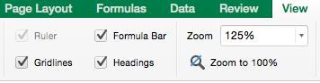
The Gridlines provide the usual reader of an Excel Workbook a level of clarity, but it is better suited for presentation purposes to someone who simply wants to review a workbook rather than modifying it.

2) How to use Format Painter in Excel

The Format Paint function can be helpful when you want to copy the formatting of a certain cell and is actually a better alternative to “Copy” and “Paste” since it is faster.

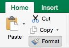
To make a cell the same format as another, click the paint brush button on the top left ribbon.

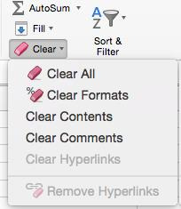
3) How to Clear Formats in Excel

You can Clear formats (font, size, gridlines, etc.) to clarify and cleanse data to its raw format. Click on the “Home” button on the top ribbon, navigate to the “Clear” button on the right side, and then click the “Clear Formats” button.

4) How to Remove Formula Errors in Excel

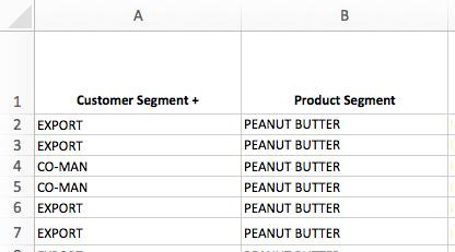
This key formatting tip is often used when using formulas like the VLOOKUP because if the VLOOKUP function does not return what you’re searching for, then it would result in an error. By inserting the function “=iferror(),0)” it will show a “0” instead of errors such as #VALUE!, #DIV/0!, etc. making it look less aggressive for someone reviewing your work.

This is also beneficial if you are calculating the sum or using other formulas on a certain set of data. If there are formula errors in that data, you won’t be able to run a formula on it but if the formula errors are removed then it won’t give a formula error when running a summation.

5) How to Insert a 0 at the beginning of a cell in Excel

Use the ‘ to insert a 0 at the beginning of a cell. This is particularly useful since 0’s generally disappear from cells regardless if you put them or not.

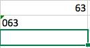
In the first row above, the 0 was written without the apostrophe, and then written with it before entering 63 on the second row, hence showing the difference.

6) How to Freeze panes in Excel

You can Freeze panes so that the viewer doesn’t have to guess or scroll back up to the header to view the header’s name or date.

Do this by going on “View” and clicking on “Freeze Panes”. The ‘Freeze Top Row’ function locks up the first row so you can view it as you scroll down back and forth anywhere on the workbook. The ‘Freeze First Column’ function similarly locks up the first column so you can view it while scrolling back and forth, right and left of it anywhere on the workbook. The following are examples the before and after effects of applying Freeze Panes.

Normal View

Freeze Panes

In the example above, the 5th row have been frozen using the ‘Freeze Panes’ option allowing me to scroll up and down, left and right while still having the view of the 4 rows above it.

Freeze Top Row

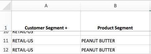
In the case above, the ‘Freeze Top Row’ option was used and it can be seen how it froze the first row while you can scroll down to the 11th and 12th rows and still have the access to it.

Freeze First Column

The ‘Freeze First Column’ option was used above and it can be seen how moving left and right does not affect the first column as it always stays fixed as a reference.

6) How to change Date Formats in Excel

It is important that you choose a date format and be consistent with it throughout a financial model. The following image illustrate the short date and long date format options.

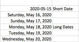
Click on date cells and format cells as dates and make a selection between the short and long date formats as shown above. The following are the different date format options in Excel. These allow users to select a date format that best fit their needs.

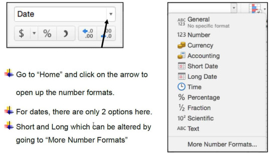
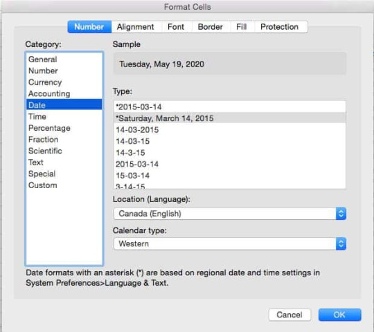
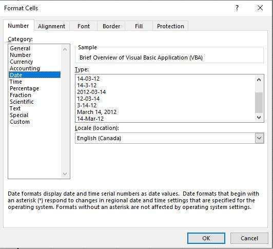
The “More Number Formats” open up the Format Cells options that list the categories for different versions of dates.

All of the formats can be selected from here, but the most professional version is on the bottom picture in the standard format of March 14, 2012.

However, different places require different formats so it is preferential.

The Format Cells also features alignment, font, border, and color fill, all of which are used for financial statements such as P&L. The benefits of these features will be discussed later in the blog

8) How to Lock Cells in Excel (Tip – Click F2 to enter cell)

Locking Cells is a good way to maintain consistency when applying formulas.

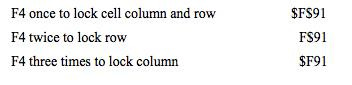
You can lock cells to avoid movement when copying formula to another cell by applying the ‘$’ before the rows and columns you want locked. ‘$’ sign before the row locks the row cell, and the ‘$’ sign before the column number locks the column.

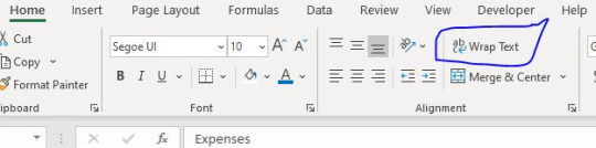
9) How to use Home/word wrap in Excel

The Word wrap text tool in Excel allows you to consolidate texts within a cell and avoid it going into the subsequent cells. Simply go “Home” and highlight the desired column, shifting the width of the desired column, and then clicking the “Wrap Text” button.

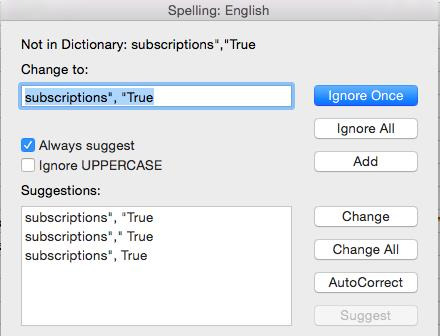
10) How to Use Review Spelling in Excel

Making spelling mistakes in any profession seems unprofessional. The spelling option in Excel is a proofreading tool that reviews for any mistakes and is the perfect tool when writing technical reports, essays, research, etc.

Simply go to the “Review” section and click on “Spelling” to check for any spelling errors. Once it opens, you can decide to ignore the word(s) and/or even change it to a suggested word from the ‘Suggestions’ box.

11) Why and How to Use “Align” in Excel

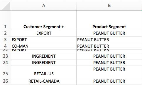
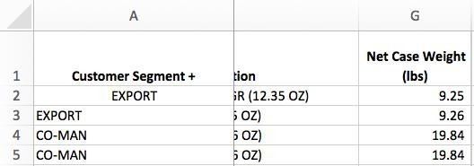
The Alignment tool in Excel is an effective way to indent cells without affecting their values or formulas. You can present subtotal data properly without inserting spaces so that formula can still be used on the cells. This can be done using the align signs for left and right from the “Alignment” section from the “Home” tab.

The following entries show the difference between the effects of an alignment change when compared to adding spaces. The first 2 formulas entered were to give the result ‘true’ if the words ‘’subscriptions’’ and “usage” matched with the text written in the quotation of each formula after the ‘=’ sign. The F43 refers to the cell in green, while F44 refers to the cell in blue. When there no changes being made, the results equate to being ‘true’ as the words clearly match.

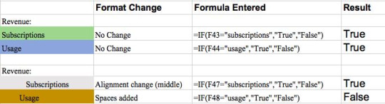
However, when we make changes in formatting using alignment using spaces, we see different result. The aligned “subscriptions” cell above in grey remains true as we used the alignment function in Excel to push the text to the right.

On the other hand, in the brown cell above for “usage” there were manual spaces added before the word “usage.” This changes the text in the cell and therefore when we run formula on the cell to lookup the word “usage” it cannot find that word in the cell and the result is false. Therefore, it is a better idea to use the alignment function in Excel as opposed to using manual spacing.

12) How to Highlight Data Table in Excel

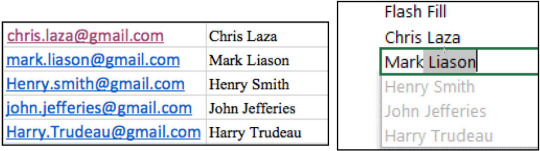
When you have a long list of client emails and need to write their names beside it, this Excel tool will help you solve this problem. In order to highlight the data table, click “Control + E”. The purpose of a flash filling is that it will automatically infer the first and last names from a list of emails if presented by that order.

14) How to Set up a P&L for Presentation?

When it comes to setting up financial models, it is important to make it look neat, organized, and professional. The following model is an example of a P&L setup with the inclusions of borders, italics, and modified rows and columns.

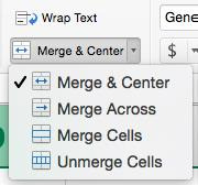
This format divides up the actual and forecasting data for revenue through 2020 for all 4 quarters. For example, you can make the top header have a color fill and use white text. You can also implement a border using the border function and choose any color, for example black. Lastly, you can also merge cells for cases like the actual and forecast section using the “Merge” button on “Home”.

15) Using the Instructions Tab in Excel

If you’re preparing a financial model, it would be beneficial to implement an instructions tab in Excel dedicated with instructions on how to update the financial model. This will allow others who open the file for review or entry to have a guideline on how to operate the workbook catered to your style.

16) Using the Assumptions Tab in Excel

Following on that, the assumptions Tab is another fundamental aspect to add to the P&L to make it more detailed and informative for the viewer as it would have a tab dedicated with key assumptions built into the financial model and make use of the variables. If you are building a financial model, it is worthwhile to have an assumption Tab as when you make changes to it, and when it gets modified, it would update the rest of the workbook. You should set it up so that the assumptions can be modified on the assumptions tab which would allow you to do this.

17) How to Summarize Data in Excel

Place the data along with the columns and summarize data into fiscal quarters and years. This is one of the best ways to organize data as it is similar to the way financial statements are prepared. Moreover, another key aspect is placing the most recent data on the right side as most people tend to read from left to right. Hence, it is best to start with the oldest data on the left side and more recent on the right side.

18) How to Highlight Cells in Excel

It’s a best practice to have standardized formats for the meaning of cells so it is well understood by the user.

It is important to limit the number of highlights you use. If you do use highlighting, make sure that you have a legend in your workbook that indicates what all the highlights mean. Furthermore, if you are building a financial model consider having all input cells/ variables filled with a specific color, for example, blue. That way the user will know that if they change the contents of a cell that is blue, it will vary the results of the financial model because it is an input cell and it has dependencies.

You can also use the yellow highlight to indicate cells that have issues or requires further investigation, or red as another example. And then all the other cells can be given another color, in this case, a clear background.

Overall, it is important to have some sort of a legend that notifies the reader of its significance and offers a clear guide as to what each color represents. It also directs people as to what colors to use when contributing to that specific workbook which ultimately creates a better flow in terms of clarity and presentation.

I hope that helps. Please leave a comment below with any questions or suggestions. For more in-depth Excel training, checkout our Ultimate Excel Training Course here. Thank you!

[gvtacademy]

Get  Advanced Excel Training Institute in Delhi, Noida – GVT Academy

Microsoft Excel is a general purpose electronic spreadsheet to use to organize, calculate, and analyze data. The task you can complete with Excel ranges from preparing a simple family budget, preparing a purchase order, create an elaborate graph/chart, or managing a complex accounting ledger for a medium size business.

 Provide Basic/Advanced Understanding of Excel, make user familiar to create formula and give platform to make good analysis and introduce Powerful tools of advance excel so that user can make advance analysis with the help of those tools. Introduction to Excel, Basic Understanding Menu and Toolbar, Introduction to different category of functions like Basics, Mathematical and Statistical, Date and Time, Logical, Lookup and References, Text and Information.

Mathematical Functions:- Sum, Sumif, Sumifs, Count, Counta, Countblank, Countif, Countifs, Average, Averagea, Averageif, Averageifs, Subtotal, Aggregate, Rand, Randbetween, Roundup, Rounddown, Round, Sumproduct

Text Functions & Data Validation:- Char, Clean, Code, Concatenate, Find, Search, Substitute, Replace, Len, Right, Left, Mid, Lower, Upper, Proper, Text, Trim, Value, Large, Small Filters (Basic, Advanced, Conditional), Sort (Ascending, Descending, Cell/ Font Color), Conditional Formatting, Data Validation, Group & Ungroup, Data split.

Statistical Function & Other Functions:- Isna, Isblank, Iserr, Iseven, Isodd, Islogical, Isytext, Max, Min, Len, Right, Left, Mid, ,Maxa, Maxifs, Median, Minifs, Mina, Vara, Correl, Geomen

Logical Functions:- And, Or, If, Iferror, Not, Nested If

Lookup & Reference Functions:- VLookup, HLookup, Index, Match, Offset, Indirect, Address, Column, Columns, Row, Rows, Choose, Arrays Concept In Lookup Formula’s, Past Special, Past link

Pivot Table and Charts, Import and Export data, Protect/Unprotect sheets/workbooks. Worksheet formatting and Print Display

Data Collection Method With Data Quality, Collaboration & Security Like Share Your Workbook On Share Drive With Quality

Analysis Single/Multidimensional Analysis, Like Three Dimensional (3D) Tables, Sensitive Analysis Like Data Table, Manual What-If Analysis, Threshold Values, Goal Seek, One-Variable Data Table, Two-Variable Data Table

Advanced Excel training course involves "Hands-on experience", we believe in practice what you preach and therefore each candidate is encouraged to practically conduct each topic that is discussed for better understanding of real-world scenar Advanced Excel. This practice of comprehensive training allows candidate to gain all the concepts and skills effectively and to later efficiently apply on their field of work.

GVT Academy is one of the best Advanced Excel training institute in Noida with 100% placement assistance. GVT Academy has well structure modules and training program designed for both students and working professionals separately. At GVT Academy Advanced Excel training is conducted during all 5 days, and special weekend classes. can also be arranged and scheduled. We also provide fast track training programs for students and professionals looking to upgrade themselves instantly.

Get in Touch:

Email: gvtacademy@gmail.com

Call: +91 9718394718

[freeudemycourses]

[FREE] Master Excel by Playing Games What you Will learn ? Most time-saving shortcut keys (Navigation, Selections, Formulas, etc.) Most useful functions (SWITCH, SUM, IF, CONCATENATE, VLOOKUP, IFERROR, etc.)

[diceforbreakfast]

Back from Hiatus

The semester is over and I’m done with my break. The d20 bug bit me again and I’ve been spending my free time knee-deep in excel, playing with values and running models of stat systems.

I just made such a convoluted excel formula that I think I learned to code by accident. 

Basically, and with entirely made up cell references:

I needed A1 to take the value of B1 and reach the sequential sum (3 = 1+2+3 = 6). I then needed it to add the value from somewhere between D1 and D5, IF E1 = any value from C1 through C5. In other words, I needed to add a formula based on one thing to another thing, but only if a reference next to that other thing was equal to another reference elsewhere in the sheet.I then needed to repeat the relationship of C1:D5 and E1 with E2, F1, and F2.

Oh, and I needed to cap the "bonus" from D1 through D5 to a maximum of 5, so I needed another formula that added up all the bonus values, summed them, subtracted 5 from that number, and then subtracted what was left from the total from the first half of the formula.

To pull this off, I had to create a series of reference cells on a hidden sheet that compared my E1, E2, F1, and F2 values with the C1:C5 range. The MATCH formula throws an error if there isn't a match, though, so I had to create a second column with IFERROR that replaced the unusable #NA from the original reference with "NM" for "No Match". My formula checks to see if *that* reference is equal to "NM" or literally anything else. 

This ugly, disgusting formula came out as:

=(C16*(C16+1)/2) -IF(AC13<>"",3,0) -IF(U13<>"",3,0) -IF(AC10<>"",3,0) +IF(Resources!H45="NM",0,VLOOKUP(Q10,L33:P38,4,FALSE)) +IF(Resources!H46="NM",0,VLOOKUP(Y10,L33:P38,4,FALSE)) +IF(Resources!H47="NM",0,VLOOKUP(Q13,L33:P38,4,FALSE)) +IF(Resources!H48="NM",0,VLOOKUP(Y13,L33:P38,4,FALSE)) -IF((+IF(Resources!H45="NM",0,VLOOKUP(Q10,L33:P38,4,FALSE)) +IF(Resources!H46="NM",0,VLOOKUP(Y10,L33:P38,4,FALSE)) +IF(Resources!H47="NM",0,VLOOKUP(Q13,L33:P38,4,FALSE)) +IF(Resources!H48="NM",0,VLOOKUP(Y13,L33:P38,4,FALSE)))>5, (+IF(Resources!H45="NM",0,VLOOKUP(Q10,L33:P38,4,FALSE)) +IF(Resources!H46="NM",0,VLOOKUP(Y10,L33:P38,4,FALSE)) +IF(Resources!H47="NM",0,VLOOKUP(Q13,L33:P38,4,FALSE)) +IF(Resources!H48="NM",0,VLOOKUP(Y13,L33:P38,4,FALSE))-5),0) &"+d20"

The italicized portion is just one giant nested IF statement.

I should probably be lil' ashamed that this is how I used my free time, but I'm honestly too proud right now that this worked.