#linear equations in one variable class 8 activity | Explore Tumblr Posts and Blogs

biomedgrid · 2 years

Text

Biomed Grid | A Random Walk Model to Evaluate the Post Transcriptional Process in Rett Syndrome

Introduction

A mental disorder is a syndrome in an individual characterized by clinically significant disorders in cognition, emotional regulation, or behavior that reflect a dysfunction in the psychological, biological, or developmental processes underlying mental functioning. Mental disorders are commonly associated with distress or disability in social, occupational or other important activities.

The diagnosis of a mental illness must be of clinical utility, leading clinicians to determine diagnoses, treatment plans and potential new treatments. There are specific criteria that must be met to diagnose mental disorders such as the following: background validators (similar genetic markers, family traits, temperament, and environmental exposure), competing validators (similar neural substrates, biomarkers, emotional and cognitive processing) and predictive validators (same clinical course - clinical history - and same response to treatment).

Neurodevelopmental disorders are a group of conditions that begin in the developmental period. These developmental disorders typically manifest themselves before the child enters school, characterized by manifestations of personal, social or other occupational activity disabilities. The spectrum of developmental disabilities ranges from specific learning limitations to deficiencies in social skills or intelligence [1, 2, 3, 4, 5, 6].

In particular, Rett syndrome is a neurodevelopmental disorder of genetic etiology, resulting from mutations in the MECP2 (methyl- CpG-binding protein 2) gene found on the X chromosome. Observation of this disease is unrelated to a specific ethnic group. It is prevalent in females, presenting one case every 10,000-20,000. The molecular rationale is that mutated MECP2 encodes a defective protein, incapacitating it to properly perform its biological function.

Thus, genes that should be inactive during specific phases of neuron development remain active, culminating in damage to the central nervous system [7, 8, 9, 10, 11, 12, 13, 14]. The aim of our work is to construct in analogy to the protein coding process. We chose a set of Rett syndrome- related mRNAs. We have used these RNA sequences to construct fractals using discrete random walks as a tool.

Materials and Methods

Inspired by the memory class random walk model, we have proposed a random walk model to construct the random fractal in analogy with the protein coding process [15, 16, 17, 18]. In this model the length of the sequences comprises the total time of the fractal construction. At each instant of time a nucellotide is read and a step is performed by the random walker. Each step performed at the instant of time depends on the entire history of the walker, i.e. it depends on the entire coded RNA sequence. Each state is retrieved equally. The probability of retrieving a past decision at the instant of time is. RNA is called ribonucleic acid. It is a linear polymeric molecule, made up of smaller units called nucleotides, nucleotides receive a dichotomous classification into purines (A and G) and pyrimidines (C and U).

Random tours have well-defined stochastic rules. It occurs as follows: the walker walks one step to the right or one step to the left, with the stochastic evolution equation given by

for the instant of time. When deciding to take a step to the right, that is, the variable σ(t+1) assumes value by stepping left, assume value -1.

The memory is formed of a set of random variables. σ_t ` for the time t’

(a) in the time: t+1, the time: t’ is randomly chosen with uniform probability 1⁄t of the set 1,2, 3,...,t.

(b) σ_(t+1) is determined stochastically by, σ_(t+1) =σ_t ` when reading a pyrimidine e σ_(t+1) =-σ_t ` when reading a purine.

In the time: t=0, the walker is in positionX_0, moves to the right when reading a purine or to the left when reading a pyrimidine, assuming the value, σ1=+1 and σ1=-1,

respectively. In the instant of time: t, the walker moves to the right when reading a purine or to the left when reading a pyrimidine, assuming the value: σt’=+1 e σt’=-1, respectively. Walker position is quantified by the stochastic evolution equation:

We have performed numerical experiments using them to obtain measurements of the following observable physics such as skewness, kurtosis, Hurst exponent, fractal dimension, information entropy, and fourth order Binder cumulative.

Skewness measures how much a distribution is deviated to the right or left from the distribution mean. It is measured by following the formula:

Kurtosis is a measure of whether the data are heavy-tailed or light-tailed relative to a normal distribution. Kurtosis is quantified according to the following stochastic equation:

The Hurst’s exponent serves to classify Anomalous diffusion can be classified as superdiffusive (H>1⁄2), normal diffusive(H=1⁄2) and subdifusive(H<1⁄2)

The fractal dimension (D) is a measure of roughness while(H) is a quantity that classifies the diffusion regimes. The fractal dimension is related to the Hurst exponent by the following equation:

in which δ is the dimension in Euclidean space in this case (δ=1). The information entropy measures the overall effect of bit variation associated with random walks. Information entropy is described by the equation:

in which Wk (x,t) is the probability distribution of finding random walkers in the position x and in the time: t [19].

Binder cumulant is a quantity widely used in the analysis of phase transition systems [20]. In our system we have analyzed the fourth order Binder cumulant in the context of the protein coding analogy according to the Rett syndrome RNA sequences employed to construct random fractals. Binder cumulant is quantified according to the formula:

We have measured these observable physics based on the RNA sequence data in the (Table 1).

Results

We have performed measurements of skewness, flatness, Hurst exponent, fractal dimension, entropy of information and fourth order Binder cumulant. In the (Figure 1), (Figure 2), (Figure 3), (Figure 4) we have presented the measurements of skewness, Hurst exponent, fractal dimension and entropy of information as a function of the label assigned to each RNA sequence presented in the (Table 1).

Table 1: Rett syndrome-related RNA sequences.

In the (Figure 1), we have presented typical mediated skewness. We have noted that for the 23 sequences analyzed, 15 show positive symmetry of the probability distribution, i.e., pyrimidines have a macroscopically outstanding effect over purines. While 8 sequences have negative skewness, therefore, in these cases purines have a macroscopically outstanding effect over pyrimidines.

Figure 1: Typical Skewness measurements for RNA sequences according to the labels shown in the table 1.

(Figure 2)& (Figure 3)show typical measurements of the Hurst exponent and fractal dimension. These quantities are inverse functions of each other as it was shown in the equation. (6). We have noted that there is no relationship between the skewness measurements shown in the (Figure 1). Besides, we have noted that random walks have a predominantly subdifusive regime characterized by typical measurements of, which are accompanied by roughness measurements in the range of (1.5Figure 3).

Figure 2: Typical Hurst exponent measurements for RNA sequences according to the labels shown in the table 1.

Figure 3: Typical fractal dimension measurements for RNA sequences according to the labels shown in the table 1.

In the (Figure 4), we have presented typical measures of information entropy. Entropy measurements are related to the Hurst exponent and the fractal dimension of the system. We have noted that the larger (smaller) the measurements observed for the Hurst exponent (the fractal dimension), the smaller the entropy variations. The largest entropy variation occurred for the sequence with ID hsa-miR-296-3p, being equal abits, which has a percentage of 39.13% purines and 60.87% pyrimidines.

Figure 4: Typical information entropy measurements for RNA sequences according to the labels shown in the table 1.

For information entropy, we have observed three typical behaviors in the construction of random walks, which are presented In the (Figure 5). In general, entropy from zero variation, ie at the beginning of nucleotide reading and grows to a point where it remains with a fixed range of bits. Entropy variations occur in three typical ways presented In the (Figure 5), (Figure 5), (Figure 5c) showing the results of entropy variation reading the RNA sequences with ID dre- -mir-146a, hsa-miR-122-3p and hsa-miR-296-3p, respectively. For the dre-mir-146a, hsa-miR-122-3p and hsa-miR-296-3p sequences the entropy exhibits sigmoid behavior with saturation points equal to and bits, accompanied by larger fractal dimension values equal to, and respectively. The dre-mir-146a sequence shows smoother growth for entropy, while the hsa-miR-122-3p sequence has more abrupt growth, as can be seen from the curve In the (Figure 5b). The entropy of the hsa-miR-296-3p sequence grows faster than the sequences of (Figure 5), (Figure 5), We have also noticed that even though curve (Figure 5) has a higher saturation point, curve (Figure 5) grows faster but stabilizes first. This fact can be explained by looking at the results In the figure 6. In the (Figure 6), the ordinary Binder cumulative measurements are presented. The term responsible for such variations is the (⟨x2⟩)2 , because according to our observations the kurtosis is invariant for all the averages that we have made, and it is equal to ⟨x4⟩=214.748. Note that, for curve (Figure 6), the Binder cumulant grows to saturation point, while curves (Figure 6), (Figure 6) have points the cumulant has a lower concave region. , then grows reaching the saturation points each. Besides, we have noticed that the bigger this region is concave, the greater the initial entropy variation, as can be seen in curves (Figure 5a & 5c), (Figure 6), (Figure 6).

Figure 5: Behavior of information entropy as a function of the number of nucleotides read in the random walk construction process for RNA sequences (a) dre-mir-146a, (b) hsa-miR-122-3p and (c) hsa-miR-296-3p.

Figure 6: Cumulative Binder behavior as a function of the number of nucleotides read in the random walk construction process for RNA sequences (a) dre-mir-146a, (b) hsa-miR-122-3p and (c) hsa -miR-296-3p.

Discussion

We have studied Rett syndrome from a stochastic perspective, performing a process of constructing fractal objects through an analogy between protein coding and random class walks with memory. This method was used to be used as a tool for analysis and diagnosis of Rett syndrome, observing some RNA sequences related to the post-transcription process responsible for protein coding. We observed that typical skewness measurements are not related in this problem as averages of Hurst exponent and fractal dimension.

Kurtosis remains invariant for all the measurements we have made. Therefore, skewness and flatness measurements are shown without any impact to extract pertinent information to analyze Rett syndrome. Furthermore, we have observed that lower Hurst exponent values are accompanied by higher fractal dimension averages (higher roughness) and greater entropy variations. Random walks present the classification of their regime as subdifusive, constructing a fractal object with the dimension between a straight line and a plane. Surprisingly, it is noted that the entropy measurements are related to the Binder cumulative measurements. The emergence of a concave region in the cumulant is related to greater variations in entropy, and the larger the concave region, the greater the variations in entropy.

Read More About this Article: https://biomedgrid.com/fulltext/volume6/a-random-walk-model-to-evaluate-the-post-transcriptional-process-in-rett-syndrome.001092.php

For more about: Journals on Biomedical Science :Biomed Grid | Current Issue

#biomedgrid #american journal of biomedical science & research #american medical journal #top medical open access journal

0 notes

learnflix · 3 years

Text

Download the NCERT Solutions for Class 8 Maths and 10 Maths PDF

School students prefer to use the best methods to learn important things every day. They are safe at home in this pandemic situation. However, they do not fail to study. They use the Internet and mobile gadgets to study from anywhere at any time. If you are a student and willing to study your class 8 maths subject without complexity in any aspect, then you can make contact with the official website of the professional learning app Learnflix. You will get instant access to the NCERT Solutions for Class 8 Maths pdf download and make a good decision to study maths. The user-friendly nature of this educational app encourages almost every user to suggest it to others. Thus, the total number of active users of this app in recent times is increased.

A good app to study maths

Many students are unable to study maths at home and searching for the best solutions to such problems. They can use one of the most recommended educational apps renowned for the ncert solutions for class 10 maths pdf download facilities. They can take note of testimonials from users of the Learnflix and decide on how to properly use this app. The main chapters in the maths for class 10 are real numbers, quadratic equations, polynomials, arithmetic progressions, pair of linear equations in two variables, coordinate geometry, triangles, and introduction to trigonometry. Students who have chosen this mobile app can study each chapter and enhance their expertise enough to score high in this subject.

For more information about best learning apps for students, for kids and free download educational app here - https://learnflix.in

Follow us on Our Social Profile Links: https://www.facebook.com/learnflixapp https://twitter.com/learnflixapp https://www.instagram.com/learnflix https://www.linkedin.com/company/learnflix2 https://play.google.com/store/apps/details?id=com.learnflix https://apps.apple.com/us/app/learnflix/id1467336078

#learning app #best learning apps #best learning app for students #class 8 maths syllabus #cbse syllabus for class 10 maths #class 9 maths syllabus #class 9 science syllabus #cbse class 7 science syllabus

0 notes

ncertsolutionsmath · 4 years

Text

Download NCERT Solutions for Class 8 Maths Chapter Wise

NCERT Solutions for Class 8 Maths incorporates all the inquiries gave in the NCERT course reading that is endorsed for Class 8 as per the CBSE Board. The schedule given by the CBSE for all the classes is totally founded on the NCERT educational plan. Henceforth, planning of tests utilizing the NCERT Solutions will give understudies a favorable position of scoring admirably.

My Way Teaching NCERT Class 8 Solutions for Maths has been intended to assist the understudies with addressing the CBSE Class 8 Maths issues effortlessly. The CBSE 8th Class Solutions for Maths gave here comes decidedly ready activities alongside definite clarifications organized by our master educators that further makes learning and comprehension of ideas a simple assignment. Thus, if understudies have been searching for the most point by point and precise NCERT Maths Solutions Class 8, which are likewise free, this is the correct spot.

Chapter Wise NCERT Solutions for Class 8 Maths NCERT Solutions Class 8 Maths provided here are very beneficial for students. They can use these NCERT Solutions for Class 8 as a reference while practising math problems and develop better math skills along with preparing efficiently for the exams. The math exercises are given at the end of every chapter to practise the concepts learned in the chapter.

NCERT Solutions for Class 8 Maths Chapter 1 Rational Numbers In this chapter, students will be learning properties related to real numbers, integers, whole numbers, rational numbers and natural numbers – independent, associative and closure. The chapter deals with the role of zero and one, multiplication over addition as well as the representation of Rational Numbers on the number line, along with searching for Rational Numbers between two Rational Numbers. The topics of additive identity (0) and multiplicative identity (1) are also covered in this chapter. There are 2 exercises in this chapter, which contain questions from all the topics present in the chapter.

NCERT Solutions for Class 8 Maths Chapter 2 Linear Equations in One Variable The chapter, Linear Equations in One Variable, deals with linear expression in one variable alone. Here the chapter will be dealing with the equations with linear expressions in one variable only. Such equations are known as Linear Equations in One Variable. There are six exercises in this chapter with a total of 65 questions in them. The chapter includes different concepts including- solving an equation of Linear Equations in One Variable, some of its applications, reducing equations to a simpler form and word problems related to Linear Equations in One Variable.

NCERT Solutions for Class 8 Maths Chapter 3 Understanding Quadrilaterals The chapter, Understanding Quadrilaterals, of Class 8 Maths, as the name says, provides the students with a proper understanding of the quadrilaterals. The chapter also covers different kinds of polygons, including triangles, quadrilaterals, pentagon, hexagon etc. The chapter contains 4 exercises which aid the students in understanding these shapes properly.

NCERT Solutions for Class 8 Maths Chapter 4 Practical Geometry The chapter, Practical Geometry, includes the method of constructing a quadrilateral with various parameters given. The chapter consists of 5 exercises, each dealing with different methods of constructing the quadrilateral. For instance, the first exercise deals with the construction of quadrilaterals when the length of four sides and a diagonal are given; similarly, the second exercise involves the method of construction of quadrilaterals when two diagonals and three sides are given, and so on. Hence, we can conclude that learning this chapter will make the students well-versed in all the concepts of quadrilateral for further classes.

NCERT Solutions for Class 8 Maths Chapter 5 Data Handling The collection of information that can be used for analysis is known as data. In this chapter, students learn about the organisation and representation of data. Organising the data in a systematic method is referred to as Data Handling. In this chapter, students learn to represent these data diagrammatically as a pictograph, a bar graph, double bar graph, pie chart and histogram. During the course of this chapter, students will be briefed about the concept of probability or likelihood. There are 3 exercises in this chapter that deal with all the concepts covered in the chapter.

NCERT Solutions for Class 8 Maths Chapter 6 Square and Square Roots This chapter, Squares and Square Roots, helps the students learn about the concept of square number and the square root of a number. The chapter deals with properties of square numbers, interesting patterns that could be learned using square numbers, finding the square of a number, Pythagorean triplets, finding square roots through various methods, Square roots of decimals and much more.

0 notes

siva3155 · 5 years

Text

300+ TOP STATA Interview Questions and Answers

STATA Interview Questions for freshers experienced :-

1. What is the elementary use of Stata? The integrated statistical software is fundamentally used as an integral part of research methodologies in the field of economics, biomedicine, and political science in order to examine data pattern. 2. What are the most advisable functions performed with the help of Stata? The program is best suited for processing time? the series, panel, and cross? sectional data. 3. What makes the tool more intuitive? The availability of both command line and graphical user interface makes the usage of the software more spontaneous. 4. What are the competencies of using Stata software? The incorporation of data management, statistical analysis, graphics, simulations, regression, and custom programming and at the same time it also accommodates a system to disseminate user-written programs that lets it grow continuously, making it an integral statistical tool. 5. List four major builds of Stata and state their purposes? STATA MP - Multiprocessor computer which includes dual-core and multicore processors. STATA SE - Majorly used for analyzing larger databases STATA IC - The standard version of the software Numerics by STATA support MP, SE AND IC data types in an embedded environment. 6. State the various disciplines which use Stata as an integral software for efficient results? STATA software acts as an effective analytical and statistical tools for major sectors, they are as follows : Behavioral sciences: Behavioral scientist entrust STATA for its accuracy, extensibility, reproducibility, and ease of use features. Whether it is an extensive research on cognitive development, studying personality traits or developing measurement instruments, The software accommodates all the required collateral to pursue a broad range of behavioral science questions. Education: In the process of developing new tests or researching diverse topics as learning and development, teacher effectiveness, or school finance, STATA establishes the relevant and accurate statistical methodology options forward. The analysis is consistently integrated with illustrations (graphics) and data management into one package in order to seek a wide range of educational questions. Medical: Medicinal researchers entrust to use STATA for its range of biostatistical methods and reproducibility approach towards the data. In the process of any medical research or while performing a clinical trial, the program provides accurate tools which helps conduct the study from power and sample-size calculations to data management to analysis. Biostatistics: Biostatisticians approve of STATA for its accuracy, extensibility, and reproducibility. Inconsiderate of the study��s statistical approach or focus area or whether it is a cross-sectional, longitudinal, or time-to-event. STATA equips the users with all the necessary statistics, graphics, and data management tools needed to implement and study a wide range of biostatistical methods. Economics: The researchers in the field of economics have always relied upon STATA for its accuracy and relevancy. Whether its a study on educational institution selection research process, Gross domestic price or stock trends, Stata provides all the statistics, graphics, and data management tools needed to complete the study with utmost authenticity. Business / Finance - Marketing: financial and marketing research analysts often rely on this tool in the case of researching asset pricing, capital market dynamics, customer-value management, consumer and firm behaviour, or branding, the reason being its accuracy and extensibility of providing all the statistics, graphics, and data management tools. Sociology: Apart from the above-listed sectors, STATA is also used in the study of demographic and geographic research processes. 7. What are the key features of Stata/ MP? STATA/ MP is termed as the fastest and largest version of the program. This version’s multiprocessing abilities provide the most comprehensive support (multi core) to all kinds of statistics and data administration. STATA/MP supports over 64 cores/processors, making it the fastest medium to analyze the data when compared to STATA/SE. This version interprets 10 to 20 billion observations in comparison to STATA/SE’s 2 billion observations. The program is 100% compatible with other versions and needs no modification of the analyses to obtain Stata/MP's speed improvements. 8. List down few highlights of new Stata 15? Extended regression modules which can address the problems such as Endogenous covariates, Nonrandom treatment assignment etc in any combination, unlike the previous Heckman and ivregress modules. STATA’S Latin Class Analysis helps to identify unobserved categories in the latent classes. STATA now supports Markdown - A standard markup language that allows text formatting from plain text input. Program's Dynamic stochastic general equilibrium command estimates the parameters of DSGE models that are linear in the variables but potentially nonlinear in the parameters. Bayes prefix, when combined with Bayesian features with STATA’S spontaneous and elegant specification of regression models, lets the users fit Bayesian regression models more conveniently and fit additional models. 9. What is the work function of Stata’S user interface? Primarily, STATA by default opens in four different windows : Results: This window displays all the commands and their results, with an exception being made for graphs which are showcased in their own window. Review: Only the commands are made visible in this particular window. When clicked on any specific command by the user it appears on a separate window. The review tab has an option of “ Save Review Contents ” which allows the user to save all documented files in the review window to a file for later use. ( This is not a substitute for log and do files.) Command: This is the space used to type the commands while working in an interactive mechanism. All the content typed here will be reflected in both results and review windows. “ Page Up “ and “ Page Down “ keys are used in order to view previously executed commands. Variables: Entire list of user ’s variables and their labels are displayed here. When clicked it will be pasted in the command window. 10. What are the various data format compatible with Stata software? STATA is compatible to import data from various formats, Inclusive of ASCII data formats (such as CSV or databank formats) and spreadsheet formats (including various Excel formats). It can as well read and write SAS XPORT format datasets natively, using the fdause and fdasave commands. The STATAS’s dominion file formats are platform independent, which enables the users from different operating systems comfortably exchange datasets and programs. Although there has been consistent change over the course of time with respect to STATA’S data format, still the users can read all older dataset formats and can write both the current and most recent previous dataset format, using the same old command.

STATA Interview Questions 11. Elaborate on Do, Log and CmdLog files? The User must always operate his work in a do-file, which ensures the output can be reproduced at a later time. One can start a do.file by simply clicking on the do.file editor button. The user has to also make sure to always turn on “Auto indent” and Auto save on do/run” options presented in the preferences tab. Another cardinal rule while working on STATA is the always maintain a log file running. These files have a record of the work done and even showcases the results. This function can be activated by giving "log using mylog.log" command. The usage of “.log” extension automatically creates the log as a plain text file that can then be opened in Microsoft Word or notepad as well as Stata's viewer. One can initiate command log with the command "cmdlog using mycmdlog.log". This ensures the file is saved in the text format. CmdLog has only the executed commands with no reflection of the output. Additionally, all the commands irrespective of where they are issued from are recorded in the command log. 12. Explain Stata salient features? Time series: This feature of the software allows the users to handle all the statistical challenges constitutional to time-series data, for example, common factors, autoregressive conditional heteroskedasticity, unit roots, autocorrelations etc. The program operates various activities like filtering to fitting compound multiple variate models and graphing which reveals the structure into the time series. Survival Analysis: With the help of specialized survival analytical tools provided by STATA, the user an analyze the duration of an outcome. They can estimate and plot the possibility of survival over time irrespective of discrepancies such as (unobserved event, delay entry or gaps in the study). hazard ratios, mean survival time, and survival probabilities can be predicted with the help of this model. Extended regression Models: ERM is the face name for the class of models addresses several complications that arise on a regular basis frequently. Example of ERMS are 1) endogenous covariates, 2) sample selection and 3) non random treatment assignment. These complications can either arise alone or with any combination. The ERMs grants the user to make authentic inferences. Structural Equation Modeling: SME performs an assessment of the mediation effects. It evaluates the relationship between unobserved latent concept and observed variables that measure the concerned latent concept. ANOVA / MANOVA: These are known as Fit one- and two-way models. They analyze the data enclosed, fixed or random factors or with repeated measures. ANOVA is used when the user faces continuous covariates, whereas MANOVA models when the user has multiple outcome variables. The relationship between the outcome and predictors can be explored by estimating effect sizes and computing least-squares and marginal means. 13. List down standards methods and advanced techniques provided by Stata program? STATA provides over 100 various authentic statistical tools. Here are the few examples: STANDARD METHODS ADVANCED TECHNIQUES Basic tabulations and summaries Time-series smoothers Multilevel models Binary, count, and censored outcomes Case-control analysis Contrasts and comparisons Dynamic panel-data (DPD) regressions Multiple imputations Power analysis SEM (structural equation modeling) ANOVA and MANOVA Latent class analysis (LCA) 14. Explain Publication - Quality graphics feature? STATA makes it convenient for the users to generate high-quality styled graphs and visual representations. A user can either point and click or write scripts to produce numerous graphs in a reproducible manner. In order to view the visual, it must be either converted into EPS or TIF for publication, to PNG or SVG for the web, or to PDF. With an additional feature of integrated graph editor, the user can alter the graph accordingly. 15. List the different graph styles provided by STATA? STATA is one of the recommended software to create graphical illustrations, the following are the types of graphs made available by STATA namely : Bar charts Box plots Histograms Spike plots Pie charts Scatterplot matrices Dot charts Line charts Area charts etc. 16. How does the reading and documentation function work in STATA? In order to write a program to read data into STATA, Then the user has two possible choices. “Infile” and “infix” . When compared to infix, the infile command has more capabilities but at the same time has a higher level of complexity. If the user’s codebook has “start” and “length” information for the variables or the variables are separated by spaces ( not commas or tabs) then it advisable to use infile. On the other hand, if the codebook contains “start” and “end” column information then, the user can go ahead with infix. 17. What are the advantages of using STATA program? STATA is a fast, accurate and easy to use interface, with an additional feature of intuitive command syntax making it a powerful statistical data analytical tool. STATA provides a wide range of statistical tools from standard methods such as Basic tabulations and summaries, Case-control analysis, Linear regression to advanced techniques for example: Multilevel models, Dynamic panel data regressions, SEM etc. Data administration feature of STATA allows complete control over all data types. The user can then combine and reshape data sets, manage variables, and collect statistics across groups or duplicates. The software is capable to manage unique data sets (survival/duration data, panel/longitudinal etc.) The program is cross-platform compatible which includes windows, MAC, Linux. 18. Explain the role of MATA programming language? MATA is a full-fledged programming language that compiles the data typed into bytecode, optimizes it, and executes it fast. Al though it is not a requirement in order to use STATA a fast and complex matrix programming language is an essential part of STATA. The language acts as both interactive environments for manipulating matrices and fully developed environment that can produce compiled and optimized code. It complies important features for the processing of panel data, performs operations on real or complex matrices and offers outright support for object-oriented -programming and is fully integrated with every form of STATA. 19. Explain describe and codebook commands? Once the data is loaded in STATA, User must document in order to know what are the variables and how they are coded. The describe and codebook commands furnish information about the user’s data. Describe command is the most basic form of a command. It projects a short description of the file and also lists variables and their required information in the datasets. Codebook drafts a detailed description of each variable. By default, the codebook command will list variables that have nine or less discrete values and means for those which are more than nine. STATA Interview Questions and Answers Pdf Download Read the full article

0 notes

juniperpublishers-biostatistics · 5 years

Text

Prediction of Strong Ground Motion Using Fuzzy Inference Systems Based on Adaptive Networks

Authored by Mostafa Allameh Zadeh*

Abstract

Peak ground acceleration (PGA) estimates have been calculated in order to predict the devastation potential resulting from earthquakes in reconstruction sites. In this research, a training algorithm based on gradient descent were developed and employed by using strong ground motion records. The Artificial Neural Networks (ANN) algorithm indicated that the fitting between the predicted strong ground motion by the networks and the observed PGA values were able to yield high correlation coefficients of 0.78 for PGA. We attempt to provide a suitable prediction of the large acceleration peak from ground gravity acceleration in different areas. Methods are defined by using fuzzy inference systems based on adaptive networks, feed-forward neural networks (FFBP)by four basic parameters as input variables which influence an earthquake in regional studied. The affected indices of an earthquake include the moment magnitude, rupture distance, fault mechanism and site class. The ANFIS network — with an average error of 0.012 — is a more precise network than FFBP neural networks. The FFBP network has a mean square error of 0.017 accordingly. Nonetheless, these two networks can have a suitable estimation of probable acceleration peaks (PGA) in this area.

Keywords: Adaptive-network-based fuzzy inference systems; Feed-forward back propagation error of a neural network; Peak ground acceleration; Rupture distance

Abbreviations: PGA: Peak ground acceleration; ANN: Artificial Neural Networks; FFBP: Feed-Forward Neural Networks; FIS: Fuzzy Inference System; Mw: Moment Magnitude

Introduction

Peak ground acceleration is a very important factor that must be considered in any construction site in order to examine the potential damage that can result from earthquakes. The actual records by seismometers at nearby stations may be considered as a basis. But a reliable method of estimation may be useful for providing more detailed information of the earthquake’s characteristics and motion [1]. The peak ground acceleration parameter is often estimated by the attenuation of relationships and also by using regression analysis. PGA is one of the most important parameters, often analyzed in studies related to damages caused by earthquakes [2]. It is mostly estimated by the attenuation of equations and is developed by a regression analysis of powerful motion data. Powerful motions relating to a ground have basic effects on the structure of that region [3]. Peak ground acceleration is mostly estimated by attenuation relationships [4]. The input variables in the constructed artificial neural network model are the magnitude, the source-to-site distance and the site’s conditions. The output is the PGA. The generalization capability of ANN algorithms was tested with the same training data. Results indicated that there is a high correlation coefficient (R2) for the fitting that is between the predicted PGA values by the networks and those of the observed ones. Furthermore, comparisons between the correlations by the ANN and the regression method showed that the ANN approach performed better than the regression. Developed ANN models can be conservatively utilized to achieve a better understanding of the input parameters and their influence, and thus reach PGA predictions.

Kerh & Chaw [1] used software calculation techniques to remove the lack of certainties in declining relations. They used the mixed gradient training algorithm of Fletcher-Reeves’ back propagation error [5]. They applied three neural network models with different inputs including epicentric distance, focal depth and magnitude of the earthquakes. These records were trained and then the output results were compared with available nonlinear regression analysis. The comparisons demonstrated that the present neural network model did have a better performance than that of the other methods. From a deterministic point of view, determining the strongest level of shaking- that can potentially happen at a site- has long been an important topic in earthquake science. Also, the maximum level of shaking defines the maximum load which ultimately affects urban structures.

From a probabilistic point of view, knowledge of the greatest ground motions that can possibly occur would allow a meaningful truncation of the distribution of ground motion residuals, and thus lead to a reduction in the computed values pertaining to probabilistic seismic hazard analyses. Particularly, it points to the low annual frequencies that exceed norms which are considered for critical facilities [6,7]. Empirical recordings of ground motions that feature large amplitudes of acceleration or velocity play a key role in defining the maximum levels of ground motion, which outline the design of engineering projects, given the potentially destructive nature of motions. They also provide valuable insights into the nature of the tails that further distribute the ground motions.

Feed-forward, back propagation error in neural networks

Artificial neural networks are a set of non-linear optimizer methods which do not need certain mathematical models in order to solve problems. In regression analysis, PGA is calculated as a function of earthquake magnitude, distance from the source of the earthquake to the site under study, local condition of the site and other characteristics that are linked to the earthquake source such as slippery length and reverse, normal or wave propagation. In non-linear regression methods, non-linear relations which exist between input and output parameters are expressed as estimations, through statistical calculations within a specified relationship [8]. One of the most popular neural networks is the back propagation algorithms. It is particularly useful for data modeling and the application of predictions [9] (Equations 1, 2 and 3). It is a supervised learning technique which was first described by Werbos [10] and further developed by Rumelhart et al. [11]. Furthermore, its most useful function is for feed forward neural networks where the information moves in one direction only, forward, beginning from the input nodes through to the hidden nodes, and then to the output nodes. There are no cycles or loops in the network.

In (1), one instance of iteration is written for the back propagation algorithm. Where Xk is a vector of current weights and biases, gk is the current gradient and a is the learning rate.

In (2), where F is the performance function of error (mean square error),'t' is the target and 'a' is the real output

In (3), 'a' is the net output,(n) is the net input and 'f' is the activation function of the neuron model

In (4), the error of energy is calculated by the least squares estimate for back-propagation learning algorithm. Where N is the number of training patterns, m is the number of neurons in the output layer. And tjk is the target value of processing the neuron. Therefore, this algorithm changes synaptic weights along with the negative gradient of the error energy function. Furthermore, it mostly benefits feed-forward neural networks where the information moves in only one direction, forward, beginning from the input nodes, through to the hidden nodes, and then to the output nodes. There are no cycles or loops in the network. The basic back-propagation algorithm adjusts the weights in the steepest direction of descent wherein the performance function decreases most rapidly. This network is a general figure of a multi-layer Prospectron network with one or several occasions of connectivity. Theoretically, it can prove every theorem that can be proven by the feed-forward network. Also, problems can be solved more accurately by testing general feed-forward networks.

Results of FFBP neural network

In Figure 1, testing the output of feed-forward neural networks against the true output is demonstrated. In Figure 2, the correlation coefficient of training, testing and validating general feed-forward neural networks is shown. In Table 1, testing the output of a feed-forward network against its true output has been compared. In Figure 3, training and validating the error graph against the feed-forward neural network is shown. Mean square error versus epoch is shown in Figure 4 with the aim of training and checking the general feed-forward

network. The sensitivity factor was obtained by training the feed-forward network (Figure 5). The sensitivity factor for input parameters is shown in Table 2. The performance error function was obtained by testing the FFBP neural network (Table 3).

Data processing

The datasets of records by large amplitude considered in this study involves one sets of accelerogram selected based on their value of PGA. These records are described below in terms of the variables generally considered to control the behavior of ground motions in general i.e. Magnitude, Rupture distance, style of faulting and site classification. The dataset includes recordings from events with Moment Magnitude ranging from (5.2-7.7) and rupture distance from (0.3-51.7 km). The SC values in the models were used as (1 to 5) for S-Wave velocity (For (1), Vs>1500 m/s and (5) Vs<180m/s). One Model was developed for each ANN method. This model was developed for estimation of maximum PGA values of the three components. The Focal Mechanism values in this model were used as (1 to 5) that (1: Strike Slip, 2:Reverse, 3:Normal, 4:Reverse oblique and 5: Normal oblique). A program includes MATLAB Neural Network toolbox was coded to train and test the models for each ANN method. All recordings from crustal events correspond to rupture distances shorter than 25km. The horizontal dataset shows a predominance of records from strike-slip and reverse earthquakes. Ground motions recorded on early strong-motions instruments often required a correction to be applied to retrieve the peak motions, Filtering generally eliminates the highest frequencies for motions recorded on modern accelerographs, and thus reduces the observed PGA values. The training of networks was performed using 60 sets of data. Testing of networks was done using 14 datasets that were randomely selected among the whole data. As shown in Figure 6 (a,b), the Mw and RD values of test and train data varied in the range of (5.2-7.7) and (0.3-52 km), respectively, the fault mechanism values were given in the Figure 6c. Figure 6d illustrated the site conditions of train and test data. As seen in this figure the site conditions were commonly soft and stiff soil types. Figure 6e showed the maximum PGA of records of the three components. In ANFIS model, training and the testing of records are shown in Figures 7a,b. Final decision surfaces are shown in Figure 7c. Final quiver surfaces are shown in Figure 7d.

Adaptive network based fuzzy inference system

The fuzzy logic appeared parallel to the growth in evolution of neural networks theory. The definition of being fuzzy can be found in human decision-making. These definitions can be searched by methods related to processing information [12].ANFIS is one of hybrid neuro-fuzzy inference expert systems and it works like the Takagi-Sugeno-type fuzzy inference system, which was developed by Jang [13]. ANFIS has a similar structure to a multilayer feed-forward neural network, but the links in an ANFIS can only indicate the flow direction of signals between nodes. No weights are associated with the links [14]. ANFIS

architecture consists of five layers of nodes. Out of the five layers, the first and the fourth layers consist of adaptive nodes while the second, third and fifth layers consist of fixed nodes. The adaptive nodes are associated with respective parameters, while the fixed nodes are devoid of any parameters [15-17]. For simplicity, we assume that the fuzzy inference system under consideration has two inputs x, y and one output called z. Supposing that the rule base contains two fuzzy if-then rules(6 and 7) of the Takagi & Sugenos [18], then the type-1 ANFIS structure can be illustrated as in Figure 6.

Rule 1: If (x is A1) and (y is B1) then (f = plx + qly + r1) (5)

Rule 2: If(x is A2) and (y is B2) then (f2 = p2 x + q2 y + r2) (6)

Where x and y are the inputs, A, Bi are the fuzzy sets and fi is the output within the fuzzy region specified by the fuzzy rule. Then pi , qiand r are the design parameters that are determined during the training process, in which a circle indicates fixed nodes, whereas a square indicates adaptive nodes.

The node functions which are in the same layer are of the same function family as described below:

In Figure 8, layer (1), every node (i) is a square node with a node function like this: O1i=μAi(x)

The outputs of this layer constitute the fuzzy membership grade of the inputs, which are presented as:

Where x and y are the inputs that enter node (i), A is a linguistic label and m (x),mBi (y) can adapt any fuzzy membership function.(a,b and c) are the parameters of the membership function. As the values of these parameters change, the bell shaped function varies accordingly. In layer 2 (Figure 8), every node is a circle node labeled n. The outputs of this layer can be presented as a firing strength of rule. In layer 3, every node is a circle node labeled N. The 'th’ node calculates the ratio of the ‘ith ’ rules' firing strength to the sum of all rules belonging to the firing strength. For convenience, outputs of this layer will be termed as normalized firing strengths. In layer 4, the defuzzification layer is an adaptive node with one node. The output of each node in this layer is simply a first order polynomial.

Where Wi is the output of layer 3, {pi * * ri} is the parameter set. Parameters in this layer will be referred to as consequent parameters. In layer 5,the summation neuron is a fixed node which computes the overall output as the summation of all incoming signals. The single node in this layer is a circle node labeled E that computes the overall output as the summation of all incoming signals.

Functionally, there are almost no constraints on the node functions of an adaptive network except in the case of a piecewise differentiability. Structurally, the only limitation of network configuration is that it should be of the feed-forward type. Due to minimal restrictions, the applications of adaptive networks are immediate and immense in various areas. In this section, we propose a class of adaptive networks which are functionally equivalent to fuzzy inference systems. The targeted architecture is referred to as ANFIS, which stands for Adaptive Network-based Fuzzy Inference System. ANFIS utilizes a strategy of hybrid training algorithm to tune all parameters. It takes a given input/output data set and constructs a fuzzy inference system which has membership function parameters that are tuned, or adjusted, using a back-propagation algorithm in combination with the least-squares type of method (NAZMY .T.M, 2009). Fuzzy inference systems are also known as fuzzy- rule-based systems, fuzzy models, fuzzy associative memories or fuzzy controllers, when used as controllers. Basically, a fuzzy inference system is comprised of five functional blocks.

a. A rule base containing a number of fuzzy if-then rules.

b. A database which defines the membership functions of the fuzzy sets used in the fuzzy rules.

c. A decision-making unit which performs inference operations on the rules.

d. A fuzzification interface which transforms the crisp inputs into degrees of match with linguistic values.

e. A defuzzification interface which transform the fuzzy results of the inference into a crisp output.

Usually the rule base and database are jointly referred to as the knowledge base. The steps of fuzzy reasoning performed by fuzzy inference systems are:

a. To compare the input variables with the membership functions on the premise part so as to obtain the membership values. (That is the fuzzification step).

b. To combine multiplications or minimizations of the membership values on the premise part so as to yield the firing strength of each rule.

c. To generate the qualified consequence— either fuzzy or crisp — of each rule depending on the firing strength.

d. To aggregate the qualified consequences so as to produce a crisp output. (That is the defuzzification step).

Results ofANFIS network for maximum PGA simulation

In this research, an adaptive neuro-fuzzy inference method was applied to simulate non-linear mapping among acceleration peak conditions. The neuro-fuzzy model included an approximate fuzzy reasoning through a sugeno fuzzy inference system (FIS). The input space was fuzzified by a grid-partitioning technique. A hybrid learning algorithm was selected in order to adapt the model's parameters. Furthermore, a linear-nonlinear regression analyses and neural network model were employed to observe the relative performances. Based on our findings, it can be concluded that the neuro-fuzzy control system exhibits a superior performance, compared to the other employed methods [19,20]. In the developed ANFIS model, input-space fuzzification was carried out via the grid-partitioning technique. Fuzzy variables were divided into four triangular membership functions *i>*2> x3* 3. The 625 fuzzy ‘if-then’ rules were set up where in the fuzzy variables were connected by the T-Norm (AND) apparatus. First order sugeno FIS was selected for the approximate reasoning process. The adjustment of independent parameters was made according to the batch mode based on the hybrid learning algorithm. The ANFIS model was trained for 50epochs until the observed error ceased to fluctuate. The resultant neuro-fuzzy Simulink model structure is illustrated in Figure 9.

The input space contains four parameters- moment magnitude (Mw), rupture distance, fault mechanism and site class. The output contains vertical components of PGA, including 40 records from different regions of the world, 24 records for training, 6 records for checking and 10 records for testing the selected ANFIS network. Sixty training data and sixty checking data pairs were obtained at first. The one used here contains 625 rules, with four membership functions being assigned to each input variable, having total number of 3185 fitting parameters which are composed of 60 premise parameters and 3125 consequent parameters. This section presents the simulation results of the proposed type-3 ANFIS with both batch (off-line) and pattern (on-line) learning. In the first example, ANFIS is used to model highly nonlinear functions, where by results are compared with the neural network approach and also with relevant earlier work. In the second example, the FIS name is PGA1 and the FIS type is sugeno. We used the 'and-or' method for input partitioning. Furthermore, we used ‘wtsum’ and 'wtaver' functions for defuzzification. The ranges of input and output variables- in other words, the target variables- are Mw=(5-8), R=(1.50-80 km), fault mechanism type =(1-5),site class=(1-5) and target range (PGA)=(0.5-2.50). The number of MFs={5 5 5 5}, the MF type=Trimf and G-bell MFs (Figure 9 $10). The result of this simulation is LSE: 0.002 and the final epoch error equals to 0.0000002.

Results of the ANFIS network

The input MFs for initial fuzzy inference system and the MFs of trained FIS are shown in Figure 11 & 12. The rule base for the designed ANFIS is shown in Figure 13. Finally, a trained FIS structure is created from the initial FIS by using the ANFIS GUI editor, which is depicted in Figure 14. Also, by testing the results, one can interpret Table 4. Fuzzy parameters used for training ANFIS are shown in Table 5. Also two membership functions for ANFIS training are shown in Figure 10.

Discussion on Results

Empirical recordings have had a significant influence on the estimation of the maximum physical ground motions that can be possible. Peak ground acceleration is an important factor which needs to be investigated before testing devastation potentials that can result from earthquakes in rebuilding sites. One of the problems that deserve attention by seismologists is the occurrence of earthquakes where of the ground motion acceleration peak unexpectedly appears to be more than 1g (Figure 15-18). Valuable data on some earthquakes have been used by Strasser [6] to investigate the earthquakes' physical processes and their consequences.

Figure 15a &b shows the acceleration and velocity traces of the horizontal components falling into this category for which the recordings were available. Spectra of pseudo-acceleration response, pertaining to damping by 5%, are also shown. All the examined traces are characterized by a very pronounced peak in the short-period (T<0.3s) range of the spectrum. The peak velocities that are associated with these recordings are less than 50cm/s. Slip distribution of focal mechanism for tohoko earthquake in Japan are shown in Figure 15c. The results of Gullo and Ercelebi's [2] research (2007) indicated that the fitting between the predicted PGA values by the networks and the observed ones yielded high correlation coefficients (R2). Furthermore, comparisons between the correlations by the ANN and the regression method showed that the ANN approach performed better than the regression method (Table 6). The developed ANN models can be used conservatively so as to establish a good understanding of the influence of input parameters for the PGA predictions.

In Strasser and Bommer's [6] research, a dataset of recordings was examined. It was characterized by the recordings' large amplitudes of PGA (1g) (Figure 15). A number of physical processes have been proposed in the literature to explain these large ground motions, which are commonly divided into source, path and site related effects. While it is often a matter of convention whether these are considered to be predominantly linked to ground motion generation (source effects) or propagation (path and site effects), particularly in the nearsource region, it is important to distinguish between factors that are event-specific, station-specific and record-specific, in terms of implications for ground motion predictions and thus seismic hazard assessment. This is because only site-specific effects can be predicted for certain, in advance. In the present paper, the ANN algorithm indicated that the fitting between the predicted PGA values by the networks and the observed PGA values could yield high correlation coefficients of 0.851for PGA ( 3). Moreover, comparisons between the correlations obtained by the ANN and the regression method demonstrated that the ANN algorithm performed better than the regressions. The Levenberg-Marquart gradient method which we applied on the training algorithm contributed dominantly to fitting the results well.

It had the potential to carry out training very quickly. Moreover, the network models developed in this paper offer new insights into attenuation studies for the purpose of estimating the PGA. In this study, ANFIS and FFBP models were developed to forecast the PGA in different regions of the world. The results of two models and the observed values were compared and evaluated based on their training and validation performance (Figures 2 & 4). The results demonstrated that ANFIS and FFBP models can be applied successfully to establish accurate and reliable PGA forecasting, when comparing the results of the two networks. It was observed that the value of R belonging to the FFBP models is high (0.78) (Figure 3). Moreover, the LSE values of the ANFIS model — which is 0.012 — were lower than that of the FFBP model (Table 4). Therefore, the ANFIS model could be more accurate than the FFBP model. However, a significant advantage is evident when predicting the PGAvia ANFIS, compared to the FFBP model (Figures 16 & 17). The simulations show that the ANFIS network is good for predicting maximum peak ground acceleration in some regions of the world. Finally, the minimum testing error- obtained for the ANFIS network- is 0.002 and the ultimate epoch error is 0.012 (Table 4). This conclusion shows that the ANFIS network can be suitable and useful for predicting values of peak ground acceleration for future earthquakes. PGA-predicted values versus record numbers for three neural networks are shown in Figure 18 & 19.

Conclusion

In this study, FFBP neural networks and ANFIS were trained so as to estimate peak ground acceleration in an area. The input variables in the ANN model were the magnitude, the rupture distance, the focal mechanism and site classification. The output was the PGA only. In the end, the minimum testing error was obtained for the ANFIS network, which equaled 0.002, and the mean square error for the FFBP neural network equaled 0.017. This conclusion shows that the ANFIS network can be suitable and useful in predicting peak ground acceleration for future earthquakes.

Acknowledgement

I am very grateful to the editors and anonymous reviewers, for their suggestions aimed at improving the quality of this manuscript. I also appreciate professors Strasser and Bommer for granting necessary data to this work.

To Know More About Biostatistics and Biometrics Open Access Journal Please Click on: https://juniperpublishers.com/bboaj/index.php

To Know More About Open Access Journals Publishers Please Click on: Juniper Publishers

#Adaptive-network #fuzzy inference systems #neural network #Rupture distance #Moment Magnitude

0 notes

aidloindia-blog · 6 years

Text

CBSE Class 11th Physics Syllabus

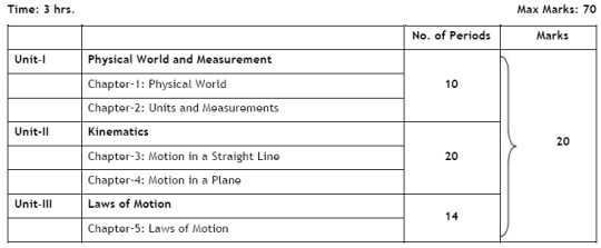
Unit I: Physical World and Measurement 10 Periods

Chapter–1: Physical World Physics-scope and excitement; nature of physical laws; Physics, technology and society. Chapter–2: Units and Measurements Need for measurement: Units of measurement; systems of units; SI units, fundamental and derived units. Length, mass and time measurements; accuracy and precision of measuring instruments; errors in measurement; significant figures. Dimensions of physical quantities, dimensional analysis and its applications.

Unit II: Kinematics 20 Periods

Chapter–3: Motion in a Straight Line Frame of reference, Motion in a straight line: Position-time graph, speed and velocity. Elementary concepts of differentiation and integration for describing motion, uniform and non-uniform motion, average speed and instantaneous velocity, uniformly accelerated motion, velocity - time and position-time graphs. Relations for uniformly accelerated motion (graphical treatment). Chapter–4: Motion in a Plane Scalar and vector quantities; position and displacement vectors, general vectors and their notations; equality of vectors, multiplication of vectors by a real number; addition and subtraction of vectors, relative velocity, Unit vector; resolution of a vector in a plane, rectangular components, Scalar and Vector product of vectors. Motion in a plane, cases of uniform velocity and uniform acceleration-projectile motion, uniform circular motion.

Unit III: Laws of Motion 14 Periods

Chapter–5: Laws of Motion Intuitive concept of force, Inertia, Newton's first law of motion; momentum and Newton's second law of motion; impulse; Newton's third law of motion. Law of conservation of linear momentum and its applications. Equilibrium of concurrent forces, Static and kinetic friction, laws of friction, rolling friction, lubrication. Dynamics of uniform circular motion: Centripetal force, examples of circular motion (vehicle on a level circular road, vehicle on a banked road).

Unit IV: Work, Energy and Power 12 Periods

Chapter–6: Work, Engery and Power Work done by a constant force and a variable force; kinetic energy, work-energy theorem, power. Notion of potential energy, potential energy of a spring, conservative forces: conservation of mechanical energy (kinetic and potential energies); non-conservative forces: motion in a vertical circle; elastic and inelastic collisions in one and two dimensions.

Unit V: Motion of System of Particles and Rigid Body 18 Periods

Chapter–7: System of Particles and Rotational Motion Centre of mass of a two-particle system, momentum conservation and centre of mass motion. Centre of mass of a rigid body; centre of mass of a uniform rod. Moment of a force, torque, angular momentum, law of conservation of angular momentum and its applications. Equilibrium of rigid bodies, rigid body rotation and equations of rotational motion, comparison of linear and rotational motions. Moment of inertia, radius of gyration, values of moments of inertia for simple geometrical objects (no derivation). Statement of parallel and perpendicular axes theorems and their applications.

Unit VI: Gravitation 12 Periods

Chapter–8: Gravitation Kepler's laws of planetary motion, universal law of gravitation. Acceleration due to gravity and its variation with altitude and depth. Gravitational potential energy and gravitational potential, escape velocity, orbital velocity of a satellite, Geo-stationary satellites.

Unit VII: Properties of Bulk Matter 20 Periods

Chapter–9: Mechanical Properties of Solids Elastic behaviour, Stress-strain relationship, Hooke's law, Young's modulus, bulk modulus, shear modulus of rigidity, Poisson's ratio; elastic energy. Chapter–10: Mechanical Properties of Fluids Pressure due to a fluid column; Pascal's law and its applications (hydraulic lift and hydraulic brakes), effect of gravity on fluid pressure. Viscosity, Stokes' law, terminal velocity, streamline and turbulent flow, critical velocity, Bernoulli's theorem and its applications. Surface energy and surface tension, angle of contact, excess of pressure across a curved surface, application of surface tension ideas to drops, bubbles and capillary rise. Chapter–11: Thermal Properties of Matter Heat, temperature, thermal expansion; thermal expansion of solids, liquids and gases, anomalous expansion of water; specific heat capacity; Cp, Cv - calorimetry; change of state - latent heat capacity. Heat transfer-conduction, convection and radiation, thermal conductivity, qualitative ideas of Blackbody radiation, Wein's displacement Law, Stefan's law, Green house effect.

Unit VIII: Thermodynamics 12 Periods

Chapter–12: Thermodynamics Thermal equilibrium and definition of temperature (zeroth law of thermodynamics), heat, work and internal energy. First law of thermodynamics, isothermal and adiabatic processes. Second law of thermodynamics: reversible and irreversible processes, Heat engine and refrigerator.

Unit IX: Behaviour of Perfect Gases and Kinetic Theory of Gases 08 Periods

Chapter–13: Kinetic Theory Equation of state of a perfect gas, work done in compressing a gas. Kinetic theory of gases - assumptions, concept of pressure. Kinetic interpretation of temperature; rms speed of gas molecules; degrees of freedom, law of equi-partition of energy (statement only) and application to specific heat capacities of gases; concept of mean free path, Avogadro's number.

Unit X: Mechanical Waves and Ray Optics 16 Periods

Chapter–14: Oscillations and Waves Periodic motion - time period, frequency, displacement as a function of time, periodic functions. Simple harmonic motion (S.H.M) and its equation; phase; oscillations of a loaded spring-restoring force and force constant; energy in S.H.M. Kinetic and potential energies; simple pendulum derivation of expression for its time period. Free, forced and damped oscillations (qualitative ideas only), resonance. Wave motion: Transverse and longitudinal waves, speed of wave motion, displacement relation for a progressive wave, principle of superposition of waves, reflection of waves, standing waves in strings and organ pipes, fundamental mode and harmonics, Beats, Doppler effect. Chapter–15: RAY OPTICS 18 Periods Ray Optics: Reflection of light, spherical mirrors, mirror formula, refraction of light, total internal reflection and its applications, optical fibres, refraction at spherical surfaces, lenses, thin lens formula, lensmaker's formula, magnification, power of a lens, combination of thin lenses in contact, refraction and dispersion of light through a prism. Scattering of light - blue colour of sky and reddish apprearance of the sun at sunrise and sunset. Optical instruments: Microscopes and astronomical telescopes (reflecting and refracting) and their magnifying powers. 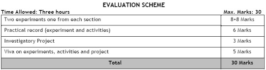The record, to be submitted by the students, at the time of their annual examination, has to include: Record of at least 15 Experiments , to be performed by the students. Record of at least 5 Activities , to be demonstrated by the teachers. Report of the project to be carried out by the students.

Activities (for the purpose of demonstration only) 1. To make a paper scale of given least count, e.g., 0.2cm, 0.5 cm 2. To determine mass of a given body using a metre scale by principle of moments 3. To plot a graph for a given set of data, with proper choice of scales and error bars 4. To measure the force of limiting friction for rolling of a roller on a horizontal plane 5. To study the variation in range of a projectile with angle of projection 6. To study the conservation of energy of a ball rolling down on an inclined plane (using a double inclined plane) 7. 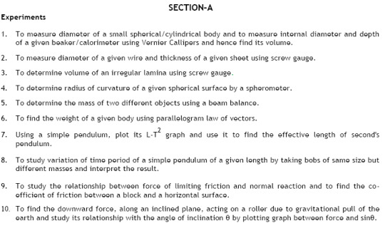To study dissipation of energy of a simple pendulum by plotting a graph between square of amplitude & time SECTION–B Experiments 1. To determine Young's modulus of elasticity of the material of a given wire. 2. To determine the surface tension of water by capillary rise method 3. To determine the coefficient of viscosity of a given viscous liquid by measuring terminal velocity of a given spherical body 4. To determine specific heat capacity of a given solid by method of mixtures 5. a) To study the relation between frequency and length of a given wire under constant tension using sonometer b) To study the relation between the length of a given wire and tension for constant frequency using sonometer. 6. To find the speed of sound in air at room temperature using a resonance tube by two resonance positions. 7. To find the value of v for different values of u in case of a concave mirror and to find the focal length. 8. To find the focal length of a convex lens by plotting graphs between u and v or between 1/u and 1/v. 9. To determine angle of minimum deviation for a given prism by plotting a graph between angle of incidence and angle of deviation. 10. To determine refractive index of a glass slab using a travelling microscope. Activities (for the purpose of demonstration only) 1. To observe change of state and plot a cooling curve for molten wax. 2. To observe and explain the effect of heating on a bi-metallic strip. 3. To note the change in level of liquid in a container on heating and interpret the observations. 4. To study the effect of detergent on surface tension of water by observing capillary rise. 5. To study the factors affecting the rate of loss of heat of a liquid. 6. To study the effect of load on depression of a suitably clamped metre scale loaded at (i) its end (ii) in the middle. 7. To observe the decrease in presure with increase in velocity of a fluid. 8. To observe refraction and lateral deviation of a beam of light incident obliquely on a glass slab. 9. To study the nature and size of the image formed by a (i) convex lens, (ii) concave mirror, on a screen by using a candle and a screen (for different distances of the candle from the lens/mirror). 10. To obtain a lens combination with the specified focal length by using two lenses from the given set of lenses.

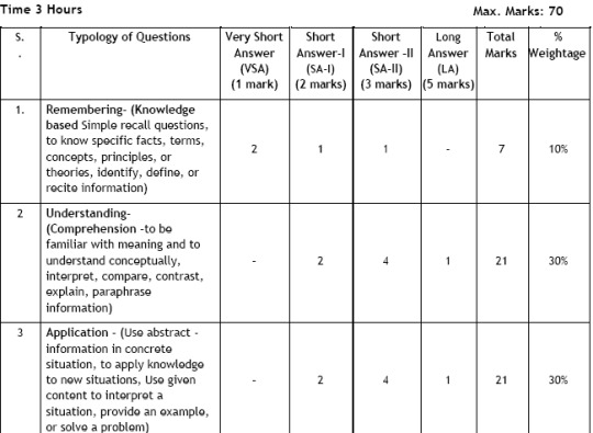
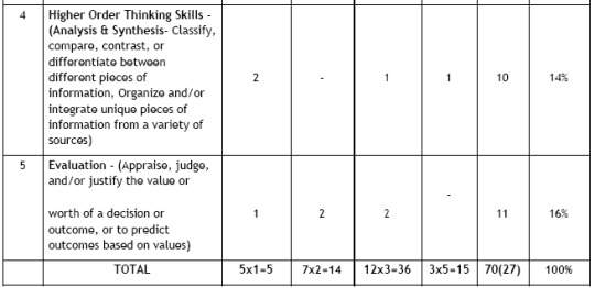
Question Wise Break Up Type of Question Mark per Question Total No. of Questions Total Marks VSA 1 5 05 SA-I 2 7 14 SA-II 3 12 36 LA 5 3 15 Total 27 70 1. Internal Choice: There is no overall choice in the paper. However, there is an internal choice in one question of 2 marks weightage, one question of 3 marks weightage and all the three questions of 5 marks weightage. 2. The above template is only a sample. Suitable internal variations may be made for generating similar templates keeping the overall weightage to different form of questions and typology of questions same. Read the full article

0 notes

studyabroadaide · 7 years

Text

UGC NET Electronic Science Books

New Post has been published on http://studyabroadaide.com/ugc-net-electronic-science-books/

UGC NET Electronic Science Books

Books Publisher 1 CBSE UGC NET/SET (NATIONAL ELIGIBILITY TEST) (STATE ELIGIBILITY TEST) ELECTRONIC SCIENCE Danika Publishing Company 2 Ugc Net Electronic Science BOOKHIVE INDIA 3 Bookhive’s Cbse Net Electronics Sciences Paper BHI EDITORIALS 4 UGC Net Electronic Science(Question Paper Book) IBS Institute Rohini

UGC NET Electronic Science Books

CBSE UGC NET/SET (NATIONAL ELIGIBILITY TEST) (STATE ELIGIBILITY TEST) ELECTRONIC SCIENCE

Ugc Net Electronic Science

Bookhive’s Cbse Net Electronics Sciences Paper

UGC Net Electronic Science(Question Paper Book)

UGC NET Electronic Science Books

UGC Net Electronic Science syllabus 2018

UNIVERSITY GRANTS COMMISSION NET BUREAU Code No. : 88 Subject: ELECTRONIC SCIENCE SYLLABUS Note: There will be two question papers, Paper—lI will cover 50 Multiple Choice Questions (Multiple choice, Matching type, True/False, Assertion-Reasoning type) carrying 100 marks and Paper-ill will have two Parts-A and B.

Part-A will have 10 short essay-type questions (300 words) carrying 16 marks each. There will be one question from each unit with internal choice from the same unit. Total marks will be 160.

Part-B will be compulsory and questions will be set from Unit—I to Unit—X. The candidate will attempt only one question from Part—B (800 words) carrying 40 marks. Total marks of Paper—iii will be 200.

PAPER-lI and III (Part A & B)

Unit—I

Electronic Transport in semiconductor, PN Junction, Diode equation and diode equivalent circuit. Breakdown in diodes, Zener diodes, Tunnel diode, Semiconductor diodes, characteristics and equivalent circuits of BJT, JFET, MOSFET, IC fabrication—crystal growth, epitaxy, oxidation, lithography, doping, etching, isolation methods, metalization, bonding, Thin film active and passive devices.

Unit—Il

Superposition, Thevenin, Norton and Maximum Power Transfer Theorems, Network elements, Network graphs, Nodal and Mesh analysis, Zero and Poles, Bode Plots, Laplace, Fourier and Z-transforms. Time and frequency domain responses. Image impedance and passive filters. Two-port Network Parameters. Transfer functions, Signal representation. State variable method of circuit analysis, AC circuit analysis, Transient analysis.

Unit—Ill

Rectifiers, Voltage regulated ICs and regulated power supply, Biasing of Bipolar junction transistors and JFET. Single stage amplifiers, Multistage amplifiers, Feedback in amplifiers, oscillators, function generators, multivibrators, Operational Amplifiers (OPAMP)—charactcristics and Applications, Computational Applications, Integrator, Differentiator, Wave shaping circuits, F to V and V to F converters. Active filters, Schmitt trigger, Phase locked loop.

Unit-TV

Logic families, ifip-flops, Gates, Boolean algebra and minimization techniques, Multivibrators and clock circuits, Counters—Ring, Ripple. Synchronous, Asynchronous, Up and down shift registers, multiplexers and demultiplexers, Arithmetic circuits, Memories, A/D and D/A converters.

Unit-V

Architecture of 8085 and 8086 Microprocessors, Addressing modes, 8085 instruction set, 8085 interrupts, Programming, Memory and 1/0 interfacing, Interfacing 8155, 8255, 8279, 8253, 8257, 8259, 8251 with 8085 Microprocessors, Serial communication protocols, Introduction of Microcontrollers (8 bit)—803 1/8051 and 8048.

Unit—VI

Introduction of High-level Programming Language, Introduction of data in C. Operators and its precedence, Various data types in C, Storage classes in C, Decision-making and forming loop in program, Handling character, Arrays in C, Structure and union, User defmed function, Pointers in C, Advanced pointer. Pointer to structures, pointer to functions, Dynamic data structure, file handling in C, Command line argument, Graphics-video modes, video adapters, Drawing various objects on screen, Interfacing to external hardware via seriallparallel port using C, Applying C to electronic circuit problems. Introduction to object-oriented Programming and C++. Introduction of FORTRAN language, programming discipline, statements to write a program, intrinsic functions, integer-type data, type statement, IF statement, Data validation, Format-directed input and output. Subscripted variables and DO loops. Array, Fortran Subprogram.

Unit—VIl

Maxwell’s equations, Time varying fields, Wave equation and its solution, Rectangular waveguide, Propagation of wave in ionosphere, Poynting vector, Antenna parameters, Half-wave antenna, Transmission lines, Characteristic of Impedance matching, Smith chart, Microwave components-T, Magic-T, Tuner. Circulator isolator, Direction couplers, Sources—Reflex Klystron, Principle of operation of Magnetron, Solid State Microwave devices; Basic Theory of Gunn, GaAs FET, Crystal Defector and PIN diode for detection of microwaves.

Unit—Ill

Basic principles of amplitude, frequency and phase modulation, Demodulation, Intermediate frequency and principle of superheterodyne receiver, Spectral analysis and signal transmission through linear systems, Random signals and noise, Noise temperature and noise figure. Basic concepts of information theory, Digital modulation and Demodulation; PM, PCM, ASK, FSK, PSK, Time-division Multiplexing, Frequency-Division Multiplexing, Data Communications—Circuits, Codes and Modems. Basic concepts of signal processing and digital filters.

Unit—IX (a)

Characteristics of solid state power devices—SCR, Triac, UJT, Triggering circuits, converters, choppers, inverters, converters. AC – regulators, speed control of a.c. and d.c. motors. Stepper and synchronous motors; Three phase controlled rectifier; Switch mode power supply; Uninterrupted power supply.

Unit—IX (b)

Optical sources—LED, Spontaneous emission, Stimulated emission, Semiconductor Diode LASER, Photodetectors—p-n photodiode. PIN photodiode, Phototransistors, Optocouplers, Solar cells, Display devices, Optical Fibres—Light propagation in fibre, Types of fibre, Characteristic parameters, Modes, Fibre splicing, Fibre optic communication system—coupling to and from the fibre, Modulation, Multiplexing and coding, Repeaters, Bandwidth and Rise time budgets.

Unit—X (a)

Transduces—Resistance, Inductance Capacitance, Peizoelectric, Thermoelectric, Hall effect, Photoelectric, Techogenerators, Measurement of displacement, velocity, acceleration, force, torque, strain, speed and sound temperature, pressure, flow, humidity, thickness, pH, position. V V Measuring Equipment—Measurement of R, L and C, Bridge and Potentiometers, voltage, current, power, energy, frequency/time, phase, DVMs, DMMs, CR0, Digital storage oscilloscope, Logic probes, Logic State Analyser, Spectrum Analyzer, Recorder, Noise and Interference in instrumentation, Instrumentation amplifiers, Radio Telemetry. Analytical Instruments—Biomedical . instruments—ECG, blood pressure measurements, spectrophotometers, Electron Microscope, X-ray diffractometer.

Unit-X (b)

Open-loop and close-loop control system. Error amplifier, on-off controller, Proportional (P), Proportional-Integral (P1), Proportional-Derivative (PD), P11) controllers, Dynamic Behaviour of control systems—servomechanism characteristics parameters of control systems—Accuracy, Sensitivity, Disturbances, Transient response, Stability, Routh-Hurwitz criterion, Bode plots, Nyquist criterion, Controlling speed. Temperature and position using analog/digital control circuits.

UGC NET Electronic Science Books

UGC Net Electronic Science syllabus 2018

0 notes