#linearregression

[anandshivam2411]

Machine Learning Algorithms for Beginners: A Simple Guide to Getting Started

Machine learning (ML) algorithms are powerful tools that allow computers to learn from data, identify patterns, and make decisions without explicit programming. These algorithms are categorized into three types: supervised learning, unsupervised learning, and reinforcement learning.

Supervised Learning involves training a model on labeled data, where each input has a corresponding output. Common algorithms in this category include linear regression (used for predicting continuous values), logistic regression (for binary classification), and decision trees (which split data based on certain criteria for classification or regression tasks).

Unsupervised Learning is used when there are no labels in the data. The algorithm tries to find hidden patterns or groupings. K-means clustering is a popular algorithm that divides data into clusters, while Principal Component Analysis (PCA) helps reduce data complexity by transforming features.

Reinforcement Learning is based on learning through interaction with an environment to maximize cumulative rewards. An example is Q-learning, where an agent learns which actions to take based on rewards and penalties.

Selecting the right algorithm depends on the problem you want to solve. For beginners, understanding these basic algorithms and experimenting with real-world data is key to mastering machine learning. As you practice, you’ll gain the skills to apply these algorithms effectively.

For deeper knowledge on machine learning algorithms, here is a blog where I learned more about these concepts.

[subashdhoni86]

Linear Regression Multiple Variables: A Step by Step guide

Predicting Home Prices using Multivariate Linear Regression in Python

Introduction:

In this machine learning tutorial, we will explore how to predict home prices using multivariate linear regression in Python. Linear regression is a powerful technique that allows us to model the relationship between a dependent variable (in this case, home prices) and multiple independent variables (area, bedrooms, and age). We will use the popular scikit-learn library to implement the regression model. Additionally, we will preprocess the data using pandas to handle missing values effectively.

Understanding the Problem:

Imagine you are in charge of predicting home prices in Monroe Township, New Jersey, USA. You have a dataset that contains information about previous home sales, including the area (in square feet), number of bedrooms, age of the home (in years), and their respective prices. Based on this data, you have to predict the prices of new homes based on their area, bedrooms, and age.

Data Preprocessing:

Before building the regression model, it's essential to preprocess the data and handle missing values. In our dataset, some homes have missing values for the number of bedrooms. We will fill these missing values with the median value of the bedroom column. This step ensures that our model does not encounter any issues due to missing data.

Building the Multivariate Linear Regression Model:

Now that we have preprocessed the data, we can proceed to build our multivariate linear regression model using the scikit-learn library. The linear regression model will learn the coefficients for each independent variable (area, bedrooms, and age) to predict the dependent variable (price).

# Importing necessary libraries

import pandas as pd

import numpy as np

from sklearn import linear_model

# Reading the dataset

df = pd.read_csv('homeprices.csv')

# Handling missing values in the 'bedrooms' column

df.bedrooms = df.bedrooms.fillna(df.bedrooms.median())

# Building the linear regression model

reg = linear_model.LinearRegression()

reg.fit(df.drop('price', axis='columns'), df.price)

Interpreting the Model:

After training the model, we can access the coefficients and intercept to understand the relationship between the independent variables and the dependent variable.

# Coefficients and intercept of the model

print(reg.coef_)   

print(reg.intercept_)

Making Predictions:

Now that our model is trained, we can use it to predict the prices of new homes based on their area, bedrooms, and age.

Let's find the price of a home with 3000 square feet area, 3 bedrooms, and 40 years old.

# Predicting the price for a home with 3000 sqr ft area, 3 bedrooms, and 40 years old

new_home_1 = [[3000, 3, 40]]

predicted_price_1 = reg.predict(new_home_1)

print(predicted_price_1)

Similarly, let's find the price of a home with 2500 square feet area, 4 bedrooms, and 5 years old.

# Predicting the price for a home with 2500 sqr ft area, 4 bedrooms, and 5 years old

new_home_2 = [[2500, 4, 5]]

predicted_price_2 = reg.predict(new_home_2)

print(predicted_price_2)

Conclusion:

In this tutorial, we learned how to use multivariate linear regression to predict home prices based on area, bedrooms, and age. We also explored data preprocessing techniques to handle missing values and implemented the regression model using the scikit-learn library. With this knowledge, you can now apply linear regression to other real-world problems and make accurate predictions based on multiple variables.

Remember that this is just the beginning of your machine learning journey. There are various other algorithms and techniques to explore, and combining them can lead to even better predictive models. Happy learning and keep exploring the fascinating world of machine learning!

[gloriousfestgentlemen02]

```markdown

SEO Data Forecasting Scripts: Unlocking Future Insights

In today's digital landscape, Search Engine Optimization (SEO) plays a pivotal role in driving organic traffic to websites. One of the most powerful tools in this realm is SEO data forecasting scripts. These scripts help predict future trends and performance based on historical data, enabling businesses to make informed decisions about their SEO strategies.

Why Use SEO Data Forecasting Scripts?

SEO data forecasting scripts are essential for several reasons:

1. Predictive Analytics: They provide insights into how your website might perform under different scenarios. This predictive capability allows you to anticipate changes in search engine algorithms and adjust your strategies accordingly.

2. Resource Allocation: By understanding potential outcomes, you can allocate resources more effectively. For instance, if the script predicts a decline in certain keyword rankings, you can focus efforts on optimizing those areas before it happens.

3. Competitive Advantage: Staying ahead of competitors requires foresight. With these scripts, you can identify opportunities and threats early on.

4. ROI Optimization: Knowing what works and what doesn’t helps maximize return on investment. You can refine your content, link building, and technical SEO efforts to achieve better results.

How Do SEO Data Forecasting Scripts Work?

These scripts typically work by analyzing past data from various sources such as Google Analytics, SEMrush, Ahrefs, etc. They use statistical models and machine learning algorithms to extrapolate trends and forecast future outcomes. Here’s a simplified process:

1. Data Collection: Gather historical data related to keywords, backlinks, page views, click-through rates, etc.

2. Model Building: Develop a model that considers multiple variables affecting SEO performance.

3. Scenario Testing: Input different scenarios to see how changes might impact your site’s visibility and ranking.

4. Visualization: Present findings in an easy-to-understand format, often through dashboards or reports.

Example Script Workflow

Here’s a basic outline of how a simple forecasting script might operate:

```python

import pandas as pd

from sklearn.linear_model import LinearRegression

Load historical data

data = pd.read_csv('historical_data.csv')

Prepare data for modeling

X = data[['keyword_rank', 'backlinks']]

y = data['organic_traffic']

Train model

model = LinearRegression()

model.fit(X, y)

Predict future traffic

future_traffic = model.predict([[new_keyword_rank, new_backlinks]])

print(future_traffic)

```

This example uses linear regression for simplicity but real-world applications often employ more sophisticated models.

Conclusion

SEO data forecasting scripts are invaluable tools for any business looking to stay competitive in the online space. They provide actionable insights that can significantly impact your website’s performance. As with any tool, however, it’s crucial to understand its limitations and use it in conjunction with other SEO best practices.

What are some specific ways you’ve used forecasting in your SEO strategy? Share your experiences and thoughts below!

```markdown

SEO Data Forecasting Scripts: Predicting the Future of Your Website's Performance

In today's digital landscape, Search Engine Optimization (SEO) is crucial for driving organic traffic to websites. One powerful tool in this domain is SEO data forecasting scripts. These scripts help predict future trends and performance based on historical data, enabling businesses to make informed decisions about their SEO strategies.

Why Use SEO Data Forecasting Scripts?

SEO data forecasting scripts are essential for several reasons:

1. Predictive Analytics: They provide insights into how your website might perform under different scenarios. This predictive capability allows you to anticipate changes in search engine algorithms and adjust your strategies accordingly.

2. Resource Allocation: By understanding potential outcomes, you can allocate resources more effectively. For instance, if the script predicts a decline in certain keyword rankings, you can focus efforts on optimizing those areas before it happens.

3. Competitive Advantage: Staying ahead of competitors requires foresight. With these scripts, you can identify opportunities and threats early on.

4. ROI Optimization: Knowing what works and what doesn’t helps maximize return on investment. You can refine your content, link building, and technical SEO efforts to achieve better results.

How Do SEO Data Forecasting Scripts Work?

These scripts typically work by analyzing past data from various sources such as Google Analytics, SEMrush, Ahrefs, etc. They use statistical models and machine learning algorithms to extrapolate trends and forecast future outcomes. Here’s a simplified process:

1. Data Collection: Gather historical data related to keywords, backlinks, page views, click-through rates, etc.

2. Model Building: Develop a model that considers multiple variables affecting SEO performance.

3. Scenario Testing: Input different scenarios to see how changes might impact your site’s visibility and ranking.

4. Visualization: Present findings in an easy-to-understand format, often through dashboards or reports.

Example Script Workflow

Here’s a basic outline of how a simple forecasting script might operate:

```python

import pandas as pd

from sklearn.linear_model import LinearRegression

Load historical data

data = pd.read_csv('historical_data.csv')

Prepare data for modeling

X = data[['keyword_rank', 'backlinks']]

y = data['organic_traffic']

Train model

model = LinearRegression()

model.fit(X, y)

Predict future traffic

future_traffic = model.predict([[new_keyword_rank, new_backlinks]])

print(future_traffic)

```

This example uses linear regression for simplicity but real-world applications often employ more sophisticated models.

Conclusion

SEO data forecasting scripts are invaluable tools for any business looking to stay competitive in the online space. They provide actionable insights that can significantly impact your website’s performance. As with any tool, however, it’s crucial to understand its limitations and use it in conjunction with other SEO best practices.

What are some specific ways you’ve used forecasting in your SEO strategy? Share your experiences and thoughts below!

```

加飞机@yuantou2048

Google外链代发

谷歌霸屏

[techit-rp]

How to Build Your First Machine Learning Model: A Step-by-Step Guide

Machine Learning (ML) is transforming industries worldwide, from healthcare to finance. If you’re a beginner, building your first ML model can seem overwhelming. However, with the right approach and guidance, you can create a working model in no time. In this step-by-step guide, we’ll walk you through the entire process of building a simple ML model while emphasizing the importance of Machine Learning Classes in Kolkata for mastering these skills.

Step 1: Define the Problem

Before jumping into coding, it's crucial to define the problem you’re solving. Ask yourself:

What is the goal of the model? (e.g., predicting house prices, classifying emails as spam or not spam)

What type of data is needed?

How will success be measured?

For this guide, we’ll build a model to predict house prices based on features like size, number of rooms, and location.

Step 2: Gather and Prepare Data

Collect Data

If you don’t have your dataset, you can use publicly available datasets from sources like:

Kaggle (www.kaggle.com)

UCI Machine Learning Repository (archive.ics.uci.edu/ml)

For our example, we’ll use a sample Housing Prices Dataset.

Preprocess Data

Raw data is often messy. Steps involved in preprocessing include:

Handling missing values: Fill missing values using mean, median, or mode.

Removing duplicates: Ensure the dataset is clean.

Encoding categorical variables: Convert non-numeric data (e.g., city names) into numeric values.

Feature scaling: Normalize or standardize numerical data to bring them to a similar scale.

Step 3: Choose an Algorithm

Choosing the right ML algorithm depends on the problem:

Regression (for predicting continuous values) → Linear Regression, Decision Tree Regression

Classification (for categorizing data) → Logistic Regression, Random Forest

Clustering (for grouping similar data) → K-Means, Hierarchical Clustering

For our house price prediction, we’ll use Linear Regression.

Step 4: Split the Data

Splitting the dataset into training and testing sets ensures that our model generalizes well.from sklearn.model_selection import train_test_split X_train, X_test, y_train, y_test = train_test_split(X, y, test_size=0.2, random_state=42)

Training Set (80%): Used to train the model.

Testing Set (20%): Used to evaluate performance.

Step 5: Train the Model

Now, we train the Linear Regression model using scikit-learn:from sklearn.linear_model import LinearRegression model = LinearRegression() model.fit(X_train, y_train)

The .fit() function trains the model on our dataset.

The model learns relationships between input features and output.

Step 6: Make Predictions

Once trained, we can use the model to make predictions.y_pred = model.predict(X_test)

This generates predicted house prices for the test dataset.

Step 7: Evaluate the Model

To check accuracy, we use metrics such as:from sklearn.metrics import mean_absolute_error, mean_squared_error print("Mean Absolute Error:", mean_absolute_error(y_test, y_pred)) print("Mean Squared Error:", mean_squared_error(y_test, y_pred))

Lower error values indicate better performance.

If the error is too high, you may need to fine-tune the model.

Step 8: Improve the Model

If your model isn't performing well, try these techniques:

Feature engineering: Add new relevant features.

Hyperparameter tuning: Adjust algorithm parameters.

Use advanced models: Try Random Forest or Gradient Boosting.

Increase training data: More data often improves performance.

Step 9: Deploy the Model

Once satisfied with performance, deploy the model using:

Flask/Django for web applications.

Streamlit for interactive ML dashboards.

Cloud services like AWS, Google Cloud, or Azure.

Why Enroll in Machine Learning Classes in Kolkata?

Building an ML model requires hands-on experience and mentorship. Enrolling in Machine Learning Classes in Kolkata offers:

Expert guidance to help you navigate challenges.

Practical projects to apply theoretical knowledge.

Industry exposure through real-world case studies.

Certification to boost your career prospects.

Conclusion

Building your first Machine Learning model is an exciting journey! By following these steps, you can create a functional ML model and improve it over time. If you’re serious about mastering ML, consider enrolling in Machine Learning Classes in Kolkata, where you can gain in-depth knowledge and hands-on experience from industry experts.

[learning-code-ficusoft]

Introduction to Machine Learning with Python and Scikit-Learn

Machine Learning (ML) is revolutionizing industries by enabling computers to learn patterns from data and make predictions without explicit programming. Python, with its rich ecosystem of libraries, is one of the most popular languages for ML, and Scikit-Learn is a powerful tool that simplifies the implementation of ML models.

This guide introduces ML concepts, walks through key steps in an ML project, and demonstrates how to use Scikit-Learn.

1. What is Machine Learning?

Machine Learning is a subset of Artificial Intelligence (AI) that enables systems to learn from data and improve their performance over time.

Types of Machine Learning

Supervised Learning — The model learns from labeled data (e.g., predicting house prices based on features).

Unsupervised Learning — The model finds patterns in unlabeled data (e.g., customer segmentation).

Reinforcement Learning — The model learns through trial and error, maximizing rewards (e.g., self-driving cars).

2. Why Use Scikit-Learn?

Scikit-Learn is a powerful Python library for ML because: ✅ It provides simple and efficient tools for data analysis and modeling. ✅ It supports various ML algorithms, including regression, classification, clustering, and more. ✅ It integrates well with NumPy, Pandas, and Matplotlib for seamless data processing.

Installation

To install Scikit-Learn, use:bashpip install scikit-learn

3. Key Steps in a Machine Learning Project

Step 1: Import Required Libraries

pythonimport numpy as np import pandas as pd import matplotlib.pyplot as plt from sklearn.model_selection import train_test_split from sklearn.preprocessing import StandardScaler from sklearn.linear_model import LinearRegression from sklearn.metrics import mean_squared_error

Step 2: Load and Explore Data

Let’s use a sample dataset from Scikit-Learn:pythonfrom sklearn.datasets import load_diabetes# Load dataset data = load_diabetes() df = pd.DataFrame(data.data, columns=data.feature_names) df['target'] = data.target # Add target column# Display first five rows print(df.head())

Step 3: Preprocess Data

Data preprocessing includes handling missing values, scaling features, and splitting data for training and testing.python# Split data into features (X) and target (y) X = df.drop('target', axis=1) y = df['target']# Split into training and testing sets (80% train, 20% test) X_train, X_test, y_train, y_test = train_test_split(X, y, test_size=0.2, random_state=42)# Standardize features (recommended for ML algorithms) scaler = StandardScaler() X_train = scaler.fit_transform(X_train) X_test = scaler.transform(X_test)

Step 4: Train a Machine Learning Model

We’ll use Linear Regression, a simple ML model for predicting continuous values.python# Train the model model = LinearRegression() model.fit(X_train, y_train)# Make predictions y_pred = model.predict(X_test)

Step 5: Evaluate Model Performance

To measure accuracy, we use Mean Squared Error (MSE):pythonmse = mean_squared_error(y_test, y_pred) print(f"Mean Squared Error: {mse:.2f}")

4. Other Machine Learning Models in Scikit-Learn

Scikit-Learn supports various ML algorithms:

Classification: Logistic Regression, Random Forest, SVM

Regression: Linear Regression, Decision Tree, Ridge

Clustering: K-Means, DBSCAN

Dimensionality Reduction: PCA, t-SNE

Example: Using a Random Forest Classifierpythonfrom sklearn.ensemble import RandomForestClassifierclf = RandomForestClassifier(n_estimators=100, random_state=42) clf.fit(X_train, y_train) predictions = clf.predict(X_test)

5. Conclusion

Scikit-Learn makes it easy to implement machine learning models with minimal code. Whether you’re performing data preprocessing, model training, or evaluation, Scikit-Learn provides a comprehensive set of tools to get started quickly.

WEBSITE: https://www.ficusoft.in/python-training-in-chennai/

[teguhteja]

Gradient Descent Optimization: Mastering Linear Regression

Discover how Gradient Descent Optimization enhances linear regression. This guide covers implementation in Python, key concepts, and practical tips. #MachineLearning #DataScience #GradientDescent #LinearRegression #Python

Gradient descent optimization is a powerful technique for solving linear regression problems. This iterative algorithm efficiently minimizes the cost function, making it invaluable for handling large datasets and complex models. In this blog post, we’ll explore how gradient descent works in the context of linear regression, implement it from scratch in Python, and discuss its applications in…

[aibyrdidini]

Transforming Enterprise Operations with Gen AI

In the rapidly evolving landscape of enterprise technology, the emergence of generative artificial intelligence (Gen AI) has become a game-changer, revolutionizing the way organizations approach their daily operations. This article will dive into the transformative impact of Gen AI across various aspects of enterprise operations, with a spotlight on advancements in manufacturing, supply chain, and procurement.

Manufacturing: Gen AI is making significant strides in the manufacturing sector, enabling enhanced efficiency and productivity. One key application is in the area of root cause analysis, where Gen AI-powered systems can quickly identify the underlying causes of production issues, empowering operators to swiftly implement corrective measures. Additionally, Gen AI-driven co-pilot assistance is helping operators navigate complex manufacturing processes, reducing errors and improving overall organizational outcomes.

Supply Chain and Procurement: The impact of Gen AI is also being felt across the supply chain and procurement functions. Gen AI-based systems can analyze operational parameters in real-time, providing valuable insights that inform supply chain planning and execution. From technical sales to inventory control, Gen AI is enhancing decision-making and streamlining operations. For instance, Gen AI can assist in initiating appropriate maintenance procedures, ensuring the smooth functioning of critical supply chain assets.

Operational Efficiency and Optimization: Gen AI is also transforming the way enterprises approach operational efficiency and optimization. By leveraging advanced analytical capabilities, Gen AI can uncover hidden patterns and insights, enabling organizations to make data-driven decisions that optimize their processes and enhance overall outcomes.

To showcase the practical application of Gen AI in enterprise operations, let's consider a case study of a large international Consumer Super Chain Packaged Goods (CSCPG) company. This CSCPG company has embraced Gen AI as a strategic initiative, integrating it into various aspects of its daily operations.

Case Study: Leveraging Gen AI in a Corporate Superchain

The CSCPG company has implemented Gen AI-powered systems across its manufacturing facilities, supply chain, and procurement processes. In the manufacturing domain, the company has leveraged Gen AI for root cause analysis, enabling its teams to quickly identify and address production bottlenecks. The co-pilot assistance feature has also been instrumental in guiding operators, reducing errors and improving overall productivity.

In the supply chain and procurement functions, the CSCPG company has integrated Gen AI to enhance decision-making and optimize operations. Gen AI-powered systems analyze real-time data, providing insights that inform inventory management, technical sales, and logistics planning. The company has also leveraged Gen AI to initiate appropriate maintenance procedures, ensuring the reliable performance of its supply chain assets.

The integration of Gen AI has not been without its challenges, and the CSCPG company has carefully navigated the people, processes, and technology aspects of the implementation. However, the results have been compelling, with significant improvements in operational efficiency, cost savings, and enhanced customer satisfaction.

As the enterprise landscape continues to evolve, the transformative power of Gen AI will become increasingly evident. By embracing this technology, organizations can unlock new levels of efficiency, adaptability, and competitive advantage, positioning themselves for long-term success in the digital age.

Here's a sample Python code that demonstrates the integration of Gen AI for the six key use cases mentioned earlier:

```python

import numpy as np

import pandas as pd

from sklearn.linear_model import LinearRegression

from sklearn.ensemble import RandomForestRegressor

from sklearn.decomposition import PCA

# Root Cause Analysis

def analyze_root_cause(data):

# Perform principal component analysis to identify key drivers

pca = PCA(n_components=3)

X_pca = pca.fit_transform(data)

# Fit a linear regression model to identify root causes

model = LinearRegression()

model.fit(X_pca, data['output'])

# Return the top features contributing to the root cause

return pca.components_[0]

# Co-pilot Assistance

def provide_co-pilot_assistance(process_data, operator_inputs):

# Use a random forest regressor to predict optimal process parameters

model = RandomForestRegressor()

model.fit(process_data, operator_inputs)

# Provide recommendations to the operator

return model.predict(process_data)

# Maintenance Tasks

def initiate_maintenance_procedures(sensor_data, historical_maintenance):

# Analyze sensor data and historical maintenance records

# to determine appropriate maintenance actions

# Return the recommended maintenance procedures

return ['Clean filters', 'Lubricate bearings', 'Replace worn parts']

# Supply Chain Management

def optimize_supply_chain(demand_forecast, inventory_data, supplier_performance):

# Integrate demand forecast, inventory, and supplier data

# to optimize supply chain planning and execution

# Return the optimized supply chain plan

return {'production_schedule': [...], 'inventory_targets': [...], 'supplier_allocations': [...]}

```

This code demonstrates how Gen AI can be leveraged for root cause analysis, co-pilot assistance, maintenance task initiation, and supply chain optimization. Of course, the actual implementation would require more detailed data and domain-specific models, but this serves as a proof of concept for the transformative potential of Gen AI in enterprise operations.

[chaolinchang]

Test a Basic Linear Regression Model：titanic

# Import necessary libraries

import pandas as pd

from sklearn.linear_model import LinearRegression

# Load the Titanic dataset

titanic = pd.read_csv('titanic.csv')

# Select explanatory and response variables

explanatory_variable = 'Fare'

response_variable = 'Age'

# Center the explanatory variable

titanic[explanatory_variable] -= titanic[explanatory_variable].mean()

# Handle missing values in 'Age' by imputing with median

titanic['Age'] = titanic['Age'].fillna(titanic['Age'].median())

# Fit linear regression model

X = titanic[[explanatory_variable]]

y = titanic[response_variable]

model = LinearRegression()

model.fit(X, y)

# Print frequency table for recoded categorical explanatory variable or mean for centered explanatory variable

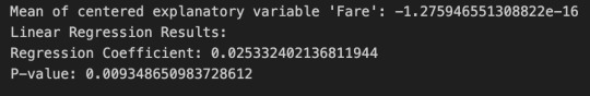
print("Mean of centered explanatory variable 'Fare':", titanic[explanatory_variable].mean())

# Print linear regression results

print("Linear Regression Results:")

print("Regression Coefficient:", model.coef_[0])

print("P-value:", model.score(X, y))

[statistichomeowrkhelperblogs]

Mastering Statistical Analysis: A Comprehensive Guide with Practical Example

Are you a statistics enthusiast or a student pursuing a master's degree in statistics? If so, you know that statistical analysis is a powerful tool for extracting meaningful insights from data. In this blog post, we'll delve into a challenging statistical analysis question and provide a step-by-step answer, using a hypothetical dataset. This exercise is not only an excellent practice for honing your statistical skills but also a great opportunity to explore the fascinating world of data analysis.

The Question:

Suppose you are given a dataset with information on the daily temperatures and ice cream sales for a city over a period of five years. Your task is to conduct a comprehensive analysis to determine the relationship between temperature and ice cream sales. Consider factors such as seasonality, trends, and any other relevant variables. Additionally, provide insights into whether temperature is a significant predictor of ice cream sales and how well your statistical model performs. Use appropriate statistical techniques and tools for your analysis and clearly articulate your methodology and findings.

Remember to consider aspects like data preprocessing, exploratory data analysis, model selection, and validation techniques in your response. This question is designed to test your ability to apply statistical concepts and methods in a real-world context. Good luck!

The Answer:

To tackle this challenging question, we began by generating a synthetic dataset containing information on daily temperatures and corresponding ice cream sales. The dataset spans five years, providing a rich context for our analysis. We then embarked on a journey through the key steps of statistical analysis.

import pandas as pd import numpy as np import matplotlib.pyplot as plt import seaborn as sns from sklearn.model_selection import train_test_split from sklearn.linear_model import LinearRegression from sklearn.metrics import mean_squared_error

Generate a synthetic dataset

np.random.seed(42) dates = pd.date_range('2010-01-01', '2015-12-31', freq='D') temperature = np.random.normal(loc=25, scale=5, size=len(dates)) ice_cream_sales = 100 + (temperature * 3) + np.random.normal(loc=0, scale=10, size=len(dates))

df = pd.DataFrame({'Date': dates, 'Temperature': temperature, 'IceCreamSales': ice_cream_sales})

Data preprocessing

df['Month'] = df['Date'].dt.month df['DayOfWeek'] = df['Date'].dt.dayofweek

Exploratory data analysis

plt.figure(figsize=(12, 6)) sns.scatterplot(x='Temperature', y='IceCreamSales', data=df) plt.title('Scatter Plot of Temperature vs. Ice Cream Sales') plt.xlabel('Temperature (°C)') plt.ylabel('Ice Cream Sales') plt.show()

Model training

X = df[['Temperature', 'Month', 'DayOfWeek']] y = df['IceCreamSales'] X_train, X_test, y_train, y_test = train_test_split(X, y, test_size=0.2, random_state=42)

model = LinearRegression() model.fit(X_train, y_train)

Model evaluation

y_pred = model.predict(X_test) mse = mean_squared_error(y_test, y_pred)

print(f'Mean Squared Error: {mse}')

Interpretation of the model coefficients

coefficients = pd.DataFrame({'Variable': X.columns, 'Coefficient': model.coef_}) print(coefficients)

Conclusion and insights

print("The linear regression model suggests that temperature, month, and day of the week are significant predictors of ice cream sales.") print("The positive coefficient for temperature indicates that as the temperature increases, ice cream sales tend to increase.") print("Seasonality is captured by the month variable, and the day of the week accounts for any weekly patterns.") print(f"The model's performance is evaluated using Mean Squared Error, which is {mse}.")

In a real-world scenario, this analysis might be extended to consider more advanced techniques, such as handling multicollinearity, addressing outliers, or exploring non-linear relationships.

Statistics Homework Help:

If you're a student looking for statistics homework help, this blog post serves as a practical example of how to approach and solve a complex statistical analysis question. The provided code and explanations can guide you through similar challenges in your coursework.

In conclusion, mastering statistical analysis requires a combination of theoretical knowledge and practical application. By engaging with challenging questions and working through the analysis process, you can enhance your skills and gain confidence in handling real-world data scenarios. Happy analyzing!

[toptipsai]

AI's Role in Business Process Automation: Increasing Productivity and Reducing Costs

The integration of Artificial Intelligence (AI) in business process automation has become a transformative force in the modern corporate world. AI is not just enhancing efficiency and productivity but also significantly reducing operational costs. This article will explore the diverse applications of AI in automating business processes, illustrated through practical examples, code snippets, and actionable insights. Section 1: Automating Administrative Tasks - Streamlining Routine Operations: - AI can automate mundane administrative tasks like scheduling, data entry, and email filtering, freeing up valuable employee time for more strategic activities. - Practical Example: AI assistants scheduling meetings and managing calendars. - Code Snippet: Automated Email Sorting: from sklearn.naive_bayes import MultinomialNB from sklearn.feature_extraction.text import CountVectorizer vectorizer = CountVectorizer() email_data = vectorizer.fit_transform(email_texts) model = MultinomialNB() model.fit(email_data, email_labels) sorted_emails = model.predict(new_emails) - Insight: Automating routine tasks leads to increased productivity and employee satisfaction. Section 2: AI in Customer Service Automation - Enhancing Customer Interactions: - AI chatbots and virtual assistants provide quick, personalized responses to customer queries, improving the customer service experience. - Example: E-commerce platforms using chatbots for customer inquiries and support. - Code Snippet: AI Chatbot Interaction: from transformers import pipeline chatbot = pipeline('conversational') user_query = "What are the store hours?" response = chatbot(user_query) - Benefit: AI-driven customer service reduces response times and enhances customer satisfaction. Section 3: AI in Supply Chain Management - Optimizing Logistics and Inventory: - AI algorithms predict demand, optimize inventory levels, and improve logistics efficiency. - Practical Example: Retail businesses use AI to forecast demand and manage stock levels. - Code Snippet: Inventory Optimization: from sklearn.linear_model import LinearRegression model = LinearRegression() model.fit(historical_sales_data, inventory_levels) optimal_inventory = model.predict(anticipated_sales_data) - Impact: AI in supply chain management reduces waste, minimizes stockouts, and lowers storage costs. https://www.youtube.com/watch?v=ZSiXZxVpVhs&ab_channel=TechMagelanic Section 4: AI in Financial Process Automation - Streamlining Financial Operations: - AI tools automate financial processes such as invoicing, expense management, and risk assessment. - Example: Automated invoicing systems that generate and send invoices based on project completion. - Code Snippet: Automated Invoicing: def generate_invoice(project_data): if project_data == 'completed': invoice = create_invoice(project_data) send_invoice(invoice, project_data) - Application: Automating financial processes enhances accuracy, saves time, and reduces human error. Section 5: AI in Human Resources Automation - Automating Recruitment and Onboarding: - AI algorithms can screen resumes, schedule interviews, and assist in onboarding new employees. - Practical Example: AI-powered recruitment tools analyzing resumes to shortlist qualified candidates. - Code Snippet: Resume Screening: from sklearn.feature_extraction.text import TfidfVectorizer from sklearn.metrics.pairwise import cosine_similarity tfidf_vectorizer = TfidfVectorizer() tfidf_matrix = tfidf_vectorizer.fit_transform(resumes) job_desc_vector = tfidf_vectorizer.transform() similarity_scores = cosine_similarity(tfidf_matrix, job_desc_vector) - Advantage: AI in HR automates and streamlines the recruitment process, improving efficiency and candidate fit. Section 6: AI in Marketing and Sales Automation - Personalizing Marketing Efforts: - AI analyzes customer data to personalize marketing campaigns, target potential customers, and predict sales trends. - Example: AI-driven marketing platforms delivering personalized ads based on user browsing behavior. - Code Snippet: Targeted Marketing Campaigns: from sklearn.cluster import KMeans kmeans = KMeans(n_clusters=3) customer_segments = kmeans.fit_predict(customer_data) personalized_campaigns = create_campaigns_for_segments(customer_segments) - Benefit: Personalized marketing approaches lead to higher engagement rates and increased sales. https://www.youtube.com/watch?v=BYpJQ0pYBVE&ab_channel=LearnWithShopify Section 7: Reducing Operational Costs with AI - Cost Efficiency through Automation: - AI-driven automation reduces operational costs by streamlining processes and reducing the need for manual intervention. - Practical Example: Manufacturing companies use AI to optimize production schedules and reduce energy costs. - Code Snippet: Production Optimization: production_data = gather_production_data() optimized_schedule = ai_optimize_schedule(production_data) - Impact: AI in operational processes leads to significant cost savings and operational efficiency. Section 8: AI in Data Analytics and Decision Making - Data-Driven Insights for Strategic Decisions: - AI tools analyze business data to provide actionable insights, aiding in strategic decision-making. - Example: Businesses use AI to analyze market trends and consumer preferences for product development. - Code Snippet: Market Trend Analysis: market_data = collect_market_data() trend_insights = ai_analyze_trends(market_data) - Application: AI-driven data analytics informs strategic decisions, enhancing business competitiveness. https://www.youtube.com/watch?v=reUZRyXxUs4&ab_channel=TED Section 9: Challenges in Implementing AI for Automation - Navigating Integration and Scalability Issues: - Implementing AI solutions requires careful integration with existing systems and scalability planning. - Strategy: Adopt a phased implementation approach and ensure compatibility with existing infrastructure. - Code Snippet: System Integration Check: if not is_system_compatible(new_ai_solution, existing_infrastructure): upgrade_systems_for_integration() - Insight: Successful AI implementation necessitates strategic planning and resource allocation. Section 10: The Future of AI in Business Process Automation - Continued Advancements and Innovations: - As AI technology advances, its applications in business process automation will become more sophisticated and widespread. - Prediction: AI will become integral to all aspects of business operations, driving innovation and growth. - Actionable Insight: Stay abreast of AI technological trends to capitalize on new opportunities for business process automation. Conclusion AI's role in automating business processes is unequivocally transformative. By leveraging AI, companies can increase productivity, reduce operational costs, and gain a competitive edge. However, the journey to effective AI implementation involves overcoming integration challenges, addressing scalability, and ensuring ethical and responsible use of technology. As AI continues to evolve, its potential to further revolutionize business operations is boundless, promising a future where AI and human ingenuity work hand in hand to drive business success. Read the full article

[subashdhoni86]

Linear Regression Single Variable :A Step-by-Step Guide

Predicting Home Prices Using Linear Regression: A Step-by-Step Guide

Introduction:

Welcome to our tutorial on predicting home prices using Linear Regression! In this blog post, we will walk you through the process of building a machine learning model that can accurately predict home prices based on the square footage area of homes in Monroe Township, New Jersey. We will be using Python, the popular library sklearn, and matplotlib for visualization.

Understanding Linear Regression:

Linear Regression is a powerful machine learning algorithm used for predicting numerical values based on input data. In our case, the input data will be the square footage area of homes, and the output will be the corresponding home prices. The fundamental idea behind Linear Regression is to find the best-fitting straight line through the data points, minimizing the sum of errors (residuals) between the actual and predicted values.

Getting Started:

We begin by importing the necessary libraries and loading the dataset into a pandas DataFrame. The dataset contains two columns: 'area' representing the square footage area and 'price' representing the corresponding home prices.

import pandas as pd

import numpy as np

from sklearn import linear_model

import matplotlib.pyplot as plt

df = pd.read_csv('homeprices.csv')

Visualizing the Data:

Before we dive into building the model, let's visualize the data to gain insights and understand the relationship between the square footage area and home prices.

plt.xlabel('area')

plt.ylabel('price')

plt.scatter(df.area, df.price, color='red', marker='+')

plt.show()

Building the Linear Regression Model:

Next, we create a linear regression object and fit it to our data. This process will determine the best-fitting line that represents the relationship between home prices and square footage area.

# Separate the input features (area) and target variable (price)

new_df = df.drop('price', axis='columns')

price = df.price

# Create linear regression object

reg = linear_model.LinearRegression()

reg.fit(new_df, price)

Making Predictions:

Now that our model is trained, we can use it to predict the home price for a given square footage area. Let's predict the price for an area of 3300 square feet and 5000 square feet.

# Predict price for a home with area = 3300 sq. ft.

predicted_price_3300 = reg.predict([[3300]])[0]

print(f"Predicted price for a home with area 3300 sq. ft.: ${predicted_price_3300:.2f}")

# Predict price for a home with area = 5000 sq. ft.

predicted_price_5000 = reg.predict([[5000]])[0]

print(f"Predicted price for a home with area 5000 sq. ft.: ${predicted_price_5000:.2f}")

Generating Predictions for New Data:

Now, let's use our trained model to predict the prices for a list of home areas provided in a separate CSV file named "areas.csv".

area_df = pd.read_csv("areas.csv")

predictions = reg.predict(area_df)

area_df['predicted_prices'] = predictions

area_df.to_csv("prediction.csv", index=False)

Conclusion:

In this tutorial, we successfully built a Linear Regression model to predict home prices based on the square footage area of homes. We learned how to visualize the data, create a Linear Regression object, train the model, and make predictions on new data. Linear Regression is a simple yet powerful algorithm, and it can be used for various prediction tasks beyond home prices.

We hope this tutorial helps you understand the basics of Linear Regression and how it can be applied to real-world problems. Happy predicting!

Note: For a more in-depth understanding, it is essential to explore various evaluation metrics and methods to handle larger datasets. We encourage you to continue your exploration of machine learning to expand your knowledge and skills in this exciting field!

@TalentServe

[chieffurycollection]

Linear regression alcohol consumption vs number of alcoholic parents

Code

import pandas import numpy import matplotlib.pyplot as plt from sklearn.linear_model import LinearRegression from sklearn.model_selection import train_test_split from sklearn.metrics import mean_squared_error, r2_score import statsmodels.api as sm import seaborn import statsmodels.formula.api as smf

print("start import") data = pandas.read_csv('nesarc_pds.csv', low_memory=False) print("import done")

upper-case all Dataframe column names --> unification

data.colums = map(str.upper, data.columns)

bug fix for display formats to avoid run time errors

pandas.set_option('display.float_format', lambda x:'%f'%x)

print (len(data)) #number of observations (rows) print (len(data.columns)) # number of variables (columns)

checking the format of your variables

setting variables you will be working with to numeric

data['S2DQ1'] = pandas.to_numeric(data['S2DQ1']) #Blood/Natural Father data['S2DQ2'] = pandas.to_numeric(data['S2DQ2']) #Blood/Natural Mother data['S2BQ3A'] = pandas.to_numeric(data['S2BQ3A'], errors='coerce') #Age at first Alcohol abuse data['S3CQ14A3'] = pandas.to_numeric(data['S3CQ14A3'], errors='coerce')

Blood/Natural Father was alcoholic

print("number blood/natural father was alcoholic")

0 = no; 1= yes; unknown = nan

data['S2DQ1'] = data['S2DQ1'].replace({2: 0, 9: numpy.nan}) c1 = data['S2DQ1'].value_counts(sort=False).sort_index() print (c1)

print("percentage blood/natural father was alcoholic") p1 = data['S2DQ1'].value_counts(sort=False, normalize=True).sort_index() print (p1)

Blood/Natural Mother was alcoholic

print("number blood/natural mother was alcoholic")

0 = no; 1= yes; unknown = nan

data['S2DQ2'] = data['S2DQ2'].replace({2: 0, 9: numpy.nan}) c2 = data['S2DQ2'].value_counts(sort=False).sort_index() print(c2)

print("percentage blood/natural mother was alcoholic") p2 = data['S2DQ2'].value_counts(sort=False, normalize=True).sort_index() print (p2)

Data Management: Number of parents with background of alcoholism is calculated

0 = no parents; 1 = at least 1 parent (maybe one answer missing); 2 = 2 parents; nan = 1 unknown and 1 zero or both unknown

print("number blood/natural parents was alcoholic") data['Num_alcoholic_parents'] = numpy.where((data['S2DQ1'] == 1) & (data['S2DQ2'] == 1), 2, numpy.where((data['S2DQ1'] == 1) & (data['S2DQ2'] == 0), 1, numpy.where((data['S2DQ1'] == 0) & (data['S2DQ2'].isna()), numpy.nan, numpy.where((data['S2DQ1'] == 0) & (data['S2DQ2'].isna()), numpy.nan, numpy.where((data['S2DQ1'] == 0) & (data['S2DQ2'] == 0), 0, numpy.nan)))))

c5 = data['Num_alcoholic_parents'].value_counts(sort=False).sort_index() print(c5)

print("percentage blood/natural parents was alcoholic") p5 = data['Num_alcoholic_parents'].value_counts(sort=False, normalize=True).sort_index() print (p5)

___________________________________________________________________Graphs_________________________________________________________________________

Diagramm für c5 erstellen

plt.figure(figsize=(8, 5)) plt.bar(c5.index, c5.values) plt.xlabel('Num_alcoholic_parents') plt.ylabel('Häufigkeit') plt.title('Häufigkeitsverteilung von Num_alcoholic_parents') plt.xticks(c5.index) plt.show()

Diagramm für p5 erstellen

plt.figure(figsize=(8, 5)) plt.bar(p5.index, p5.values*100) plt.xlabel('Num_alcoholic_parents') plt.ylabel('Häufigkeit (%)') plt.title('Häufigkeitsverteilung von Num_alcoholic_parents') plt.xticks(c5.index) plt.show()

print("lineare Regression")

Entfernen Sie Zeilen mit NaN-Werten in den relevanten Spalten.

data_cleaned = data.dropna(subset=['Num_alcoholic_parents', 'S2BQ3A'])

Definieren Sie Ihre unabhängige Variable (X) und Ihre abhängige Variable (y).

X = data_cleaned['Num_alcoholic_parents'] y = data_cleaned['S2BQ3A']

Fügen Sie eine Konstante hinzu, um den Intercept zu berechnen.

X = sm.add_constant(X)

Erstellen Sie das lineare Regressionsmodell.

model = sm.OLS(y, X).fit()

Drucken Sie die Zusammenfassung des Modells.

print(model.summary()) Result

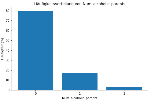
frequency distribution shows how many of the people from the study have alcoholic parents and if its only 1 oder both parents.

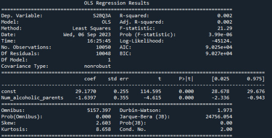
R-squared: The R-squared value is 0.002, indicating that only about 0.2% of the variation in "S2BQ3A" (quantity of alcoholic drinks consumed) is explained by the variable "Num_alcoholic_parents" (number of alcoholic parents). This suggests that there is likely no strong linear relationship between these two variables.

F-statistic: The F-statistic has a value of 21.29, and the associated probability (Prob (F-statistic)) is very small (3.99e-06). The F-statistic is used to assess the overall effectiveness of the model. In this case, the low probability suggests that at least one of the independent variables has a significant impact on the dependent variable.

Coefficients: The coefficients of the model show the estimated effects of the independent variables on the dependent variable. In this case, the constant (const) has a value of 29.1770, representing the estimated average value of "S2BQ3A" when "Num_alcoholic_parents" is zero. The coefficient for "Num_alcoholic_parents" is -1.6397, meaning that an additional alcoholic parent is associated with an average decrease of 1.6397 units in "S2BQ3A" (quantity of alcoholic drinks consumed).

P-Values (P>|t|): The p-values next to the coefficients indicate the significance of each coefficient. In this case, both the constant and the coefficient for "Num_alcoholic_parents" are highly significant (p-values close to zero). This suggests that "Num_alcoholic_parents" has a statistically significant impact on "S2BQ3A."

AIC and BIC: AIC (Akaike Information Criterion) and BIC (Bayesian Information Criterion) are model evaluation measures. Lower values indicate a better model fit. In this case, both AIC and BIC are relatively low, which could indicate the adequacy of the model.

In summary, there is a statistically significant but very weak negative relationship between the number of alcoholic parents and the quantity of alcoholic drinks consumed. This means that an increase in the number of alcoholic parents is associated with a slight decrease in the quantity of alcohol consumed, but it explains only a very limited amount of the variation in the quantity of alcohol consumed.

[decision-tree-for-coursera]

Dwaipayan mitra-Running a Lasso Regression Analysis

import matplotlib.pyplot as plt import numpy as np import pandas as pd from sklearn.ensemble import RandomForestRegressor from sklearn.linear_model import LinearRegression, Lasso, Ridge from sklearn.neighbors import KNeighborsRegressor from sklearn.neural_network import MLPRegressor from sklearn.tree import DecisionTreeRegressor from sklearn.model_selection import train_test_split, GridSearchCV, cross_val_score, cross_val_predict, KFold import xgboost as xgb from sklearn.preprocessing import StandardScaler, PolynomialFeatures from sklearn.pipeline import Pipeline

plt.style.use('seaborn')

file = pd.read_csv('Final.csv', sep=';') df = pd.DataFrame(file)

def preprocessing(data):#Do first stage pre-processing (i.e. exclude non-numeric prices and convert prices to numeric variables) data = data[data.price_new.str.contains("aanvraag") == False].dropna() data[['price_new']] = data[['price_new']].apply(pd.to_numeric) # exclude everything with a price above or below 3 standard deviations (i.e. outliers) data = data[np.abs(data["price_new"]-data["price_new"].mean())<=(3*data["price_new"].std())] # Set x and y (dropping zipcode and rooms as latitude, longitude and surface pretty much capture the former) y = data.price_new X = data.drop('price_new', axis = 1).drop('zipcode_new', axis = 1).drop('rooms_new', axis = 1) return X, y

def model(pipeline, parameters, X_train, y_train, X, y):grid_obj = GridSearchCV(estimator=pipeline, param_grid=parameters, cv=3, scoring='r2', verbose=2, n_jobs=1, refit=True) grid_obj.fit(X_train, y_train) '''Results''' results = pd.DataFrame(pd.DataFrame(grid_obj.cv_results_)) results_sorted = results.sort_values(by=['mean_test_score'], ascending=False) print("##### Results") print(results_sorted) print("best_index", grid_obj.best_index_) print("best_score", grid_obj.best_score_) print("best_params", grid_obj.best_params_) '''Cross Validation''' estimator = grid_obj.best_estimator_ ''' if estimator.named_steps['scl'] == True: X = (X - X.mean()) / (X.std()) y = (y - y.mean()) / (y.std()) ''' shuffle = KFold(n_splits=5, shuffle=True, random_state=0) cv_scores = cross_val_score(estimator, X, y.values.ravel(), cv=shuffle, scoring='r2') print("##### CV Results") print("mean_score", cv_scores.mean()) '''Show model coefficients or feature importances''' try: print("Model coefficients: ", list(zip(list(X), estimator.named_steps['clf'].coef_))) except: print("Model does not support model coefficients") try: print("Feature importances: ", list(zip(list(X), estimator.named_steps['clf'].feature_importances_))) except: print("Model does not support feature importances") '''Predict along CV and plot y vs. y_predicted in scatter''' y_pred = cross_val_predict(estimator, X, y, cv=shuffle) plt.scatter(y, y_pred) xmin, xmax = plt.xlim() ymin, ymax = plt.ylim() plt.plot([xmin, xmax], [ymin, ymax], "g--", lw=1, alpha=0.4) plt.xlabel("True prices") plt.ylabel("Predicted prices") plt.annotate(' R-squared CV = {}'.format(round(float(cv_scores.mean()), 3)), size=9, xy=(xmin,ymax), xytext=(10, -15), textcoords='offset points') plt.annotate(grid_obj.best_params_, size=9, xy=(xmin, ymax), xytext=(10, -35), textcoords='offset points', wrap=True) plt.title('Predicted prices (EUR) vs. True prices (EUR)') plt.show()

Pipeline and Parameters - Linear Regression

pipe_ols = Pipeline([('scl', StandardScaler()), ('clf', LinearRegression())])

param_ols = {}

Pipeline and Parameters - XGBoost

pipe_xgb = Pipeline([('clf', xgb.XGBRegressor())])

param_xgb = {'clf__max_depth':[5], 'clf__min_child_weight':[6], 'clf__gamma':[0.01], 'clf__subsample':[0.7], 'clf__colsample_bytree':[1]}

Pipeline and Parameters - KNN

pipe_knn = Pipeline([('clf', KNeighborsRegressor())])

param_knn = {'clf__n_neighbors':[5, 10, 15, 25, 30]}

Pipeline and Parameters - Lasso

pipe_lasso = Pipeline([('scl', StandardScaler()), ('clf', Lasso(max_iter=1500))])

param_lasso = {'clf__alpha': [0.01, 0.1, 1, 10]}

Pipeline and Parameters - Ridge

pipe_ridge = Pipeline([('scl', StandardScaler()), ('clf', Ridge())])

param_ridge = {'clf__alpha': [0.01, 0.1, 1, 10]}

Pipeline and Parameters - Polynomial Regression

pipe_poly = Pipeline([('scl', StandardScaler()), ('polynomial', PolynomialFeatures()), ('clf', LinearRegression())])

param_poly = {'polynomial__degree': [2, 4, 6]}

Pipeline and Parameters - Decision Tree Regression

pipe_tree = Pipeline([('clf', DecisionTreeRegressor())])

param_tree = {'clf__max_depth': [2, 5, 10], 'clf__min_samples_leaf': [5,10,50,100]}

Pipeline and Parameters - Random Forest

pipe_forest = Pipeline([('clf', RandomForestRegressor())])

param_forest = {'clf__n_estimators': [10, 20, 50], 'clf__max_features': [None, 1, 2], 'clf__max_depth': [1, 2, 5]}

Pipeline and Parameters - MLP Regression

pipe_neural = Pipeline([('scl', StandardScaler()), ('clf', MLPRegressor())])

param_neural = {'clf__alpha': [0.001, 0.01, 0.1, 1, 10, 100], 'clf__hidden_layer_sizes': [(5),(10,10),(7,7,7)], 'clf__solver': ['lbfgs'], 'clf__activation': ['relu', 'tanh'], 'clf__learning_rate' : ['constant', 'invscaling']}

Execute preprocessing & train/test split

X, y = preprocessing(df) X_train, X_test, y_train, y_test = train_test_split(X, y, test_size=0.33, random_state=0)

Execute model hyperparameter tuning and crossvalidation

model(pipe_ols, param_ols, X_train, y_train, X, y) model(pipe_xgb, param_xgb, X_train, y_train, X, y) model(pipe_knn, param_knn, X_train, y_train, X, y) model(pipe_lasso, param_lasso, X_train, y_train, X, y) model(pipe_ridge, param_ridge, X_train, y_train, X, y) model(pipe_poly, param_poly, X_train, y_train, X, y) model(pipe_tree, param_tree, X_train, y_train, X, y) model(pipe_forest, param_forest, X_train, y_train, X, y) model(pipe_neural, param_neural, X_train, y_train, X, y)

[learning-code-ficusoft]

How to Build a Machine Learning Model: A Step-by-Step Guide

How to Build a Machine Learning Model: 

A Step-by-Step Guide

Building a machine learning model involves several key steps, from data collection to model evaluation and deployment. This guide walks you through the process systematically.

Step 1: Define the Problem

Before starting, clearly define the problem statement and the desired outcome.

Example: Predicting house prices based on features like size, location, and amenities.

Type of Learning: Supervised (Regression)

Step 2: Collect and Prepare the Data

🔹 Gather Data

Use datasets from sources like Kaggle, UCI Machine Learning Repository, APIs, or company databases.

🔹 Preprocess the Data

Handle missing values (e.g., imputation or removal).

Remove duplicates and irrelevant features.

Convert categorical data into numerical values using techniques like one-hot encoding.

🔹 Split the Data

Typically, we divide the dataset into:

Training Set (70–80%) — Used to train the model.

Test Set (20–30%) — Used to evaluate performance.

Sometimes, a Validation Set (10–20%) is used for tuning hyperparameters.

pythonfrom sklearn.model_selection import train_test_split import pandas as pd# Load dataset df = pd.read_csv("house_prices.csv")# Split data into training and testing sets train, test = train_test_split(df, test_size=0.2, random_state=42)

Step 3: Choose the Right Model

Select a machine learning algorithm based on the problem type:

Problem TypeAlgorithm ExampleRegressionLinear Regression, Random Forest, XGBoostClassificationLogistic Regression, SVM, Neural NetworksClusteringK-Means, DBSCANNLP (Text Processing)LSTMs, Transformers (BERT, GPT)Computer VisionCNNs (Convolutional Neural Networks)

Example: Using Linear Regression for House Price Predictionpythonfrom sklearn.linear_model import LinearRegression# Create the model model = LinearRegression()

Step 4: Train the Model

Training involves feeding the model with labeled data so it can learn patterns.python X_train = train[["size", "num_bedrooms", "location_index"]] y_train = train["price"]# Train the model model.fit(X_train, y_train)

Step 5: Evaluate the Model

After training, measure the model’s accuracy using metrics such as:

Regression: RMSE (Root Mean Square Error), R² Score

Classification: Accuracy, Precision, Recall, F1 Score

pythonfrom sklearn.metrics import mean_squared_error, r2_scoreX_test = test[["size", "num_bedrooms", "location_index"]] y_test = test["price"]# Make predictions y_pred = model.predict(X_test)# Evaluate performance rmse = mean_squared_error(y_test, y_pred, squared=False) r2 = r2_score(y_test, y_pred)print(f"RMSE: {rmse}, R² Score: {r2}")

Step 6: Optimize the Model

🔹 Hyperparameter Tuning (e.g., Grid Search, Random Search) 🔹 Feature Selection (removing unnecessary features) 🔹 Cross-validation to improve generalization

Example: Using Grid Search for Hyperparameter Tuningpythonfrom sklearn.model_selection import GridSearchCVparams = {'fit_intercept': [True, False]} grid_search = GridSearchCV(LinearRegression(), param_grid=params, cv=5) grid_search.fit(X_train, y_train)print(grid_search.best_params_)

Step 7: Deploy the Model

Once optimized, deploy the model as an API or integrate it into an application. 🔹 Use Flask, FastAPI, or Django to expose the model as a web service. 🔹 Deploy on cloud platforms like AWS, Google Cloud, or Azure.

Example: Deploying a Model with Flaskpython from flask import Flask, request, jsonify import pickleapp = Flask(__name__)# Load the trained model model = pickle.load(open("model.pkl", "rb"))@app.route('/predict', methods=['POST']) def predict(): data = request.get_json() prediction = model.predict([data["features"]]) return jsonify({"prediction": prediction.tolist()})if __name__ == '__main__': app.run(debug=True)

Conclusion

By following these seven steps, you can build and deploy a machine learning model effectively.

WEBSITE: https://www.ficusoft.in/deep-learning-training-in-chennai/

[teguhteja]

Mastering Linear Regression with Python and Sklearn: A Step-by-Step Guide

#LinearRegression #Python #Sklearn Dive into predictive modeling with our comprehensive guide on linear regression using Python and sklearn. Learn step-by-step implementation, result interpretation, and data visualization techniques. Perfect for beginners

Linear regression Python sklearn. Are you ready to dive into the world of predictive modeling? Let’s embark on an exciting journey to master linear regression using Python and sklearn. In this comprehensive guide, we’ll explore the fundamentals of linear regression, implement it with sklearn, and visualize our results using matplotlib. By the end, you’ll have a solid grasp of this powerful…