#linearregression line
Explore tagged Tumblr posts
Visit Tumblr Blog
Explore Tumblr blogs with no restrictions, modern design and the best experience.
Last Seen Tumblr Blogs


Fun Fact
There are dozens of funny blogs to kill time on Tumblr.
Text
Cours des maths.Scatter plots, line of best fit.9th Grade
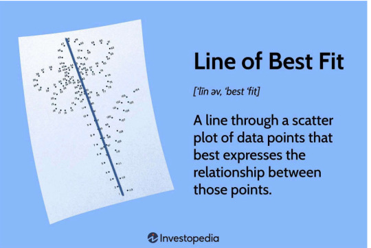
While useful for estimates, remember that a line of best fit is not perfect, and correlation doesn't always mean one variable causes the other.Check it now from here.
0 notes
Text
Data Analysis + Machine Learning Using Python (Made Simple)
Hey data lovers 👋 – ever wondered how Netflix recommends your next show, or how businesses know what you might buy next?
✨ The answer: Data Analysis + Machine Learning 🛠️ The tool: Python (yes, the programming language, not the snake 🐍)
Let’s break it down (no jargon, just vibes):
🧩 What is Data Analysis?
Data Analysis is like being a detective for numbers. You ask questions like:
What’s selling the most?
Where are customers coming from?
Why are profits dipping?
With Python, you can read spreadsheets (Excel, CSV), clean messy data, and find hidden patterns — all with just a few lines of code!
🤖 What is Machine Learning?
Machine Learning is when you teach your computer to learn from data and make predictions. Like:
📬 Spam email detector
🎥 Movie recommendations
📈 Predicting next month’s sales
Python makes all of this super doable with cool libraries like scikit-learn, TensorFlow, and PyTorch.
🧰 Favorite Python Tools:
Here’s your starter pack:
pandas – for reading and wrangling data
numpy – for numbers & math
matplotlib / seaborn – for plotting charts
scikit-learn – for training machine learning models
🔁 How It Works:
Load your data
import pandas as pd df = pd.read_csv("data.csv")
Clean it up
df.dropna(inplace=True)
Visualize it
import seaborn as sns sns.histplot(df["sales"])
Train a model
from sklearn.linear_model import LinearRegression model = LinearRegression() model.fit(X_train, y_train)
Predict the future 🔮
model.predict(X_test)
It’s that chill.
🚀 Why You Should Care:
Companies are hiring data folks like crazy
You can automate boring stuff
It’s fun to make your own smart tools
Python is beginner-friendly & free!
🌍 Real-World Magic with Python:
Detecting disease with X-rays
Building recommendation engines
Forecasting business trends
Cleaning Twitter data for sentiment analysis
🧠 Wanna Start?
Try this:
Install Jupyter Notebook
Learn Python basics (Codecademy, W3Schools)
Grab a dataset from Kaggle
Build something small (like predicting movie ratings)
🔗 In a world full of data, Python is your superpower. Start small, stay curious, and let the data speak. 💬📈
1 note
·
View note
Text
Popular python libraries for training machine learning models

There are several popular Python libraries for training machine learning models, including:
1. NumPy: A popular library for multi-dimensional array and matrix processing, often used for mathematical operations.
2. Scikit-learn: A library for machine learning algorithms, including classification, regression, and clustering.
3. Pandas: A library for data manipulation and analysis, often used for data preprocessing.
4. TensorFlow: A library for numerical computations and machine learning, often used for deep learning.
5. Keras: A high-level neural networks API, often used for building and training deep learning models.
6. PyTorch: A library for machine learning and deep learning, often used for natural language processing and computer vision.
7. Matplotlib: A library for data visualization, often used for plotting graphs and charts.
8. Theano: A library for numerical computations and machine learning, often used for deep learning.
9. Seaborn: A library for data visualization, often used for statistical graphics.
10. SciPy: A library for scientific and technical computing, often used for optimization and signal processing.

These libraries provide a range of functionalities for machine learning tasks, including data preprocessing, model selection, hyperparameter tuning, and evaluation. Developers can choose the appropriate libraries based on their specific needs and preferences.
The snippet code in Phyton as POC for Popular Python libraries for training machine learning models.
Scikit-learn is a popular library for machine learning in Python that provides simple and efficient tools for data mining and data analysis.
In this example, we will use the scikit-learn library to train a simple linear regression model on a synthetic dataset.
```python
import numpy as np
import matplotlib.pyplot as plt
from sklearn.linear_model import LinearRegression
# Generate synthetic dataset
n = 100
x = np.random.rand(n)
y = 2 * x + 1 + np.random.rand(n)
# Create a linear regression model
model = LinearRegression()
# Train the model on the synthetic dataset
model.fit(x[:, np.newaxis], y)
# Plot the data points and the regression line
plt.scatter(x, y)
plt.plot(x, model.predict(x[:, np.newaxis]))
plt.show()
# Print the coefficients of the regression model
print("Coefficients:", model.coef_)
print("Intercept:", model.intercept_)
```
In this code, we first generate a synthetic dataset by randomly generating `n` data points and adding some random noise to the `y` values. We then create a `LinearRegression` model from the scikit-learn library and train it on the synthetic dataset using the `fit` method.

We then plot the data points and the regression line using matplotlib and print the coefficients and intercept of the regression model.
RDIDINI PROMPT ENGINEER
0 notes
Text
CS Homework 1 Solution
CS Homework 1 Solution
Note: You are expected to submit both a report and code. For your code, please include clear README files. When not specifically mentioned, use the default data provided in our program package. “########## Please Fill Missing Lines Here ##########” is used where input from you is needed. 1. Linear Regression In LinearRegression\linearRegression.py, fill in the missing lines in the python code…

View On WordPress
0 notes
Text
Regression Coefficients
Regression Coefficients #TheBookOfWhy #LinearRegression
Statistical regression is a great thing. We can generate a scatter plot, generate a line of best fit, and measure how well that line describes the relationship between the individual points within the data. The better the line fits (the more that individual points stick close to the line) the better the line describes the relationships and trends in our data. However, this doesn’t mean that the…
View On WordPress
0 notes
Photo

Linear Regression tries to find parameters of the linear function, so the distance between the all the points and the line is as small as possible. Algorithms used for parameters update are called Gradient Descent. #deeplearning,#linearregression,#neuralnetworks,#machinelearning,#artificialintelligence,#regression,#numpy,#matplotlib,#pandas.#pyplot,#dataanalysis,#visualisingdata,#Initialization,#Prediction ,#datascience,#parameters,#CNN https://www.incegna.com/post/a-lenient-journey-from-linear-regression-to-neural-networks Check our Info : www.incegna.com Reg Link for Programs : http://www.incegna.com/contact-us Follow us on Facebook : www.facebook.com/INCEGNA/? Follow us on Instagram : https://www.instagram.com/_incegna/ For Queries : [email protected] https://www.instagram.com/p/B7pnGzega5I/?igshid=y6ojacoru230
#deeplearning#linearregression#neuralnetworks#machinelearning#artificialintelligence#regression#numpy#matplotlib#pandas#pyplot#dataanalysis#visualisingdata#initialization#prediction#datascience#parameters#cnn
0 notes
Text
Here’s how I used Python to build a regression model using an e-commerce dataset
The programming language of Python is gaining popularity among SEOs for its ease of use to automate daily, routine tasks. It can save time and generate some fancy machine learning to solve more significant problems that can ultimately help your brand and your career. Apart from automations, this article will assist those who want to learn more about data science and how Python can help.
In the example below, I use an e-commerce data set to build a regression model. I also explain how to determine if the model reveals anything statistically significant, as well as how outliers may skew your results.
I use Python 3 and Jupyter Notebooks to generate plots and equations with linear regression on Kaggle data. I checked the correlations and built a basic machine learning model with this dataset. With this setup, I now have an equation to predict my target variable.
Before building my model, I want to step back to offer an easy-to-understand definition of linear regression and why it’s vital to analyzing data.
What is linear regression?
Linear regression is a basic machine learning algorithm that is used for predicting a variable based on its linear relationship between other independent variables. Let’s see a simple linear regression graph:
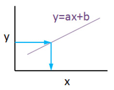
If you know the equation here, you can also know y values against x values. ‘’a’’ is coefficient of ‘’x’’ and also the slope of the line, ‘’b’’ is intercept which means when x = 0, b = y.
My e-commerce dataset
I used this dataset from Kaggle. It is not a very complicated or detailed one but enough to study linear regression concept.
If you are new and didn’t use Jupyter Notebook before, here is a quick tip for you:
Launch the Terminal and write this command: jupyter notebook
Once entered, this command will automatically launch your default web browser with a new notebook. Click New and Python 3.

Now it is time to use some fancy Python codes.
Importing libraries
import matplotlib.pyplot as plt import numpy as np import pandas as pd from sklearn.linear_model import LinearRegression from sklearn.model_selection import train_test_split from sklearn.metrics import mean_absolute_error import statsmodels.api as sm from statsmodels.tools.eval_measures import mse, rmse import seaborn as sns pd.options.display.float_format = '{:.5f}'.format import warnings import math import scipy.stats as stats import scipy from sklearn.preprocessing import scale warnings.filterwarnings('ignore')
Reading data
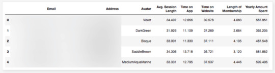
df = pd.read_csv("Ecom_Customers.csv") df.head()

My target variable will be Yearly Amount Spent and I’ll try to find its relation between other variables. It would be great if I could be able to say that users will spend this much for example, if Time on App is increased 1 minute more. This is the main purpose of the study.
Exploratory data analysis
First let’s check the correlation heatmap:
df_kor = df.corr() plt.figure(figsize=(10,10)) sns.heatmap(df_kor, vmin=-1, vmax=1, cmap="viridis", annot=True, linewidth=0.1)
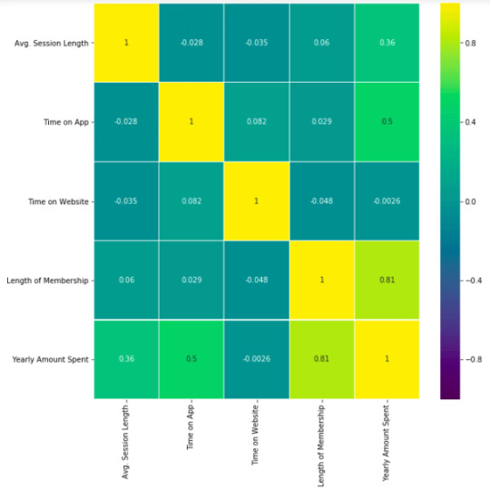
This heatmap shows correlations between each variable by giving them a weight from -1 to +1.
Purples mean negative correlation, yellows mean positive correlation and getting closer to 1 or -1 means you have something meaningful there, analyze it. For example:
Length of Membership has positive and high correlation with Yearly Amount Spent. (81%)
Time on App also has a correlation but not powerful like Length of Membership. (50%)
Let’s see these relations in detailed. My favorite plot is sns.pairplot. Only one line of code and you will see all distributions.
sns.pairplot(df)
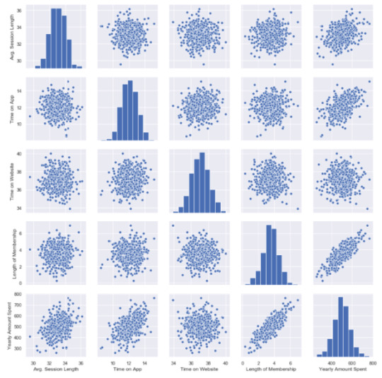
This chart shows all distributions between each variable, draws all graphs for you. In order to understand which data they include, check left and bottom axis names. (If they are the same, you will see a simple distribution bar chart.)
Look at the last line, Yearly Amount Spent (my target on the left axis) graphs against other variables.
Length of Membership has really perfect linearity, it is so obvious that if I can increase the customer loyalty, they will spend more! But how much? Is there any number or coefficient to specify it? Can we predict it? We will figure it out.
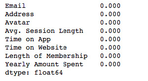
Checking missing values
Before building any model, you should check if there are any empty cells in your dataset. It is not possible to keep on with those NaN values because many machine learning algorithms do not support data with them.
This is my code to see missing values:
df.isnull().sum()

isnull() detects NaN values and sum() counts them.
I have no NaN values which is good. If I had, I should have filled them or dropped them.
For example, to drop all NaN values use this:
df.dropna(inplace=True)
To fill, you can use fillna():
df["Time on App"].fillna(df["Time on App"].mean(), inplace=True)
My suggestion here is to read this great article on how to handle missing values in your dataset. That is another problem to solve and needs different approaches if you have them.
Building a linear regression model
So far, I have explored the dataset in detail and got familiar with it. Now it is time to create the model and see if I can predict Yearly Amount Spent.
Let’s define X and Y. First I will add all other variables to X and analyze the results later.
Y=df["Yearly Amount Spent"] X=df[[ "Length of Membership", "Time on App", "Time on Website", 'Avg. Session Length']]
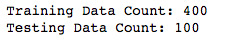
Then I will split my dataset into training and testing data which means I will select 20% of the data randomly and separate it from the training data. (test_size shows the percentage of the test data – 20%) (If you don’t specify the random_state in your code, then every time you run (execute) your code, a new random value is generated and training and test datasets would have different values each time.)
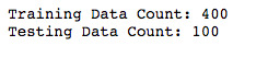
X_train, X_test, y_train, y_test = train_test_split(X, Y, test_size = 0.2, random_state = 465) print('Training Data Count: {}'.format(X_train.shape[0])) print('Testing Data Count: {}'.format(X_test.shape[0]))

Now, let’s build the model:
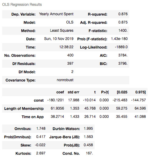
X_train = sm.add_constant(X_train) results = sm.OLS(y_train, X_train).fit() results.summary()
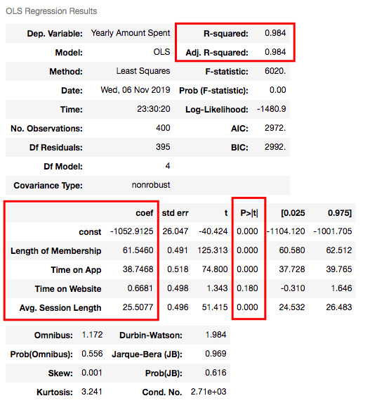
Understanding the outputs of the model: Is this statistically significant?
So what do all those numbers mean actually?
Before continuing, it will be better to explain these basic statistical terms here because I will decide if my model is sufficient or not by looking at those numbers.
What is the p-value?
P-value or probability value shows statistical significance. Let’s say you have a hypothesis that the average CTR of your brand keywords is 70% or more and its p-value is 0.02. This means there is a 2% probability that you would see CTRs of your brand keywords below %70. Is it statistically significant? 0.05 is generally used for max limit (95% confidence level), so if you have p-value smaller than 0.05, yes! It is significant. The smaller the p-value is, the better your results!
Now let’s look at the summary table. My 4 variables have some p-values showing their relations whether significant or insignificant with Yearly Amount Spent. As you can see, Time on Website is statistically insignificant with it because its p-value is 0.180. So it will be better to drop it.
What is R squared and Adjusted R squared?
R square is a simple but powerful metric that shows how much variance is explained by the model. It counts all variables you defined in X and gives a percentage of explanation. It is something like your model capabilities.
Adjusted R squared is also similar to R squared but it counts only statistically significant variables. That is why it is better to look at adjusted R squared all the time.
In my model, 98.4% of the variance can be explained, which is really high.
What is Coef?
They are coefficients of the variables which give us the equation of the model.
So is it over? No! I have Time on Website variable in my model which is statistically insignificant.
Now I will build another model and drop Time on Website variable:
X2=df[["Length of Membership", "Time on App", 'Avg. Session Length']] X2_train, X2_test, y2_train, y2_test = train_test_split(X2, Y, test_size = 0.2, random_state = 465) print('Training Data Count:', X2_train.shape[0]) print('Testing Data Count::', X2_test.shape[0])
X2_train = sm.add_constant(X2_train) results2 = sm.OLS(y2_train, X2_train).fit() results2.summary()
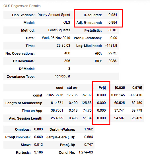
R squared is still good and I have no variable having p-value higher than 0.05.
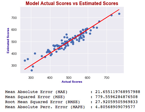
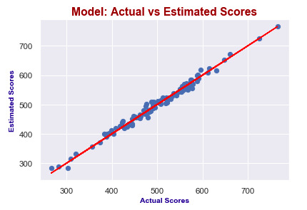
Let’s look at the model chart here:
X2_test = sm.add_constant(X2_test) y2_preds = results2.predict(X2_test) plt.figure(dpi = 75) plt.scatter(y2_test, y2_preds) plt.plot(y2_test, y2_test, color="red") plt.xlabel("Actual Scores", fontdict=ex_font) plt.ylabel("Estimated Scores", fontdict=ex_font) plt.title("Model: Actual vs Estimated Scores", fontdict=header_font) plt.show()

It seems like I predict values really good! Actual scores and predicted scores have almost perfect linearity.
Finally, I will check the errors.
Errors
When building models, comparing them and deciding which one is better is a crucial step. You should test lots of things and then analyze summaries. Drop some variables, sum or multiply them and again test. After completing the series of analysis, you will check p-values, errors and R squared. The best model will have:
P-values smaller than 0.05
Smaller errors
Higher adjusted R squared
Let’s look at errors now:
print("Mean Absolute Error (MAE) : {}".format(mean_absolute_error(y2_test, y2_preds))) print("Mean Squared Error (MSE) : {}".format(mse(y2_test, y2_preds))) print("Root Mean Squared Error (RMSE) : {}".format(rmse(y2_test, y2_preds))) print("Root Mean Squared Error (RMSE) : {}".format(rmse(y2_test, y2_preds))) print("Mean Absolute Perc. Error (MAPE) : {}".format(np.mean(np.abs((y2_test - y2_preds) / y2_test)) * 100))
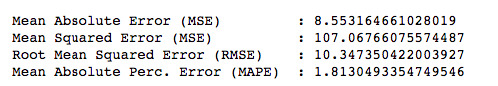
If you want to know what MSE, RMSE or MAPE is, you can read this article.
They are all different calculations of errors and now, we will just focus on smaller ones while comparing different models.
So, in order to compare my model with another one, I will create one more model including Length of Membership and Time on App only.
X3=df[['Length of Membership', 'Time on App']] Y = df['Yearly Amount Spent'] X3_train, X3_test, y3_train, y3_test = train_test_split(X3, Y, test_size = 0.2, random_state = 465) X3_train = sm.add_constant(X3_train) results3 = sm.OLS(y3_train, X3_train).fit() results3.summary()

X3_test = sm.add_constant(X3_test) y3_preds = results3.predict(X3_test) plt.figure(dpi = 75) plt.scatter(y3_test, y3_preds) plt.plot(y3_test, y3_test, color="red") plt.xlabel("Actual Scores", fontdict=eksen_font) plt.ylabel("Estimated Scores", fontdict=eksen_font) plt.title("Model Actual Scores vs Estimated Scores", fontdict=baslik_font) plt.show() print("Mean Absolute Error (MAE) : {}".format(mean_absolute_error(y3_test, y3_preds))) print("Mean Squared Error (MSE) : {}".format(mse(y3_test, y3_preds))) print("Root Mean Squared Error (RMSE) : {}".format(rmse(y3_test, y3_preds))) print("Mean Absolute Perc. Error (MAPE) : {}".format(np.mean(np.abs((y3_test - y3_preds) / y3_test)) * 100))
Which one is best?
As you can see, errors of the last model are higher than the first one. Also adjusted R squared is decreased. If errors were smaller, then we would say the last one is better – independent of R squared. Ultimately, we choose smaller errors and higher R squared. I’ve just added this second one to show you how you can compare the models and decide which one is the best.
Now our model is this:
Yearly Amount Spent = -1027.28 + 61.49x(Length of Membership) + 38.76x(Time on App) + 25.48x(Avg. Session Length)
This means, for example, if we can increase the length of membership 1 year more and holding all other features fixed, one person will spend 61.49 dollars more!
Advanced tips: Outliers and nonlinearity
When you are dealing with the real data, generally things are not that easy. To find linearity or more accurate models, you may need to do something else. For example, if your model isn’t accurate enough, check for outliers. Sometimes outliers can mislead your results!
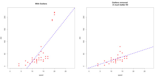
Source: http://r-statistics.co/Outlier-Treatment-With-R.html
Apart from this, sometimes you will get curved lines instead of linear but you will see that there is also a relation between variables!
Then you should think of transforming your variables by using logarithms or square.
Here is a trick for you to decide which one to use:

Source: https://courses.lumenlearning.com/boundless-algebra/chapter/graphs-of-exponential-and-logarithmic-functions/
For example, in the third graph, if you have a line similar to the green one, you should consider using logarithms in order to make it linear!
There are lots of things to do so testing all of them is really important.
Conclusion
If you like to play with numbers and advance your data science skill set, learn Python. It is not a very difficult programming language to learn, and the statistics you can generate with it can make a huge difference in your daily work.
Google Analytics, Google Ads, Search Console… Using these tools already offers tons of data, and if you know the concepts of handling data accurately, you will get very valuable insights from them. You can create more accurate traffic forecasts, or analyze Analytics data such as bounce rate, time on page and their relations with the conversion rate. At the end of the day, it might be possible to predict the future of your brand. But these are only a few examples.
If you want to go further in linear regression, check my Google Page Speed Insights OLS model. I’ve built my own dataset and tried to predict the calculation based on speed metrics such as FCP (First Contentful Paint), FMP (First Meaningful Paint) and TTI (Time to Interactive).
In closing, blend your data, try to find correlations and predict your target. Hamlet Batista has a great article about practical data blending. I strongly recommend it before building any regression model.
The post Here’s how I used Python to build a regression model using an e-commerce dataset appeared first on Search Engine Land.
Here’s how I used Python to build a regression model using an e-commerce dataset published first on https://likesfollowersclub.tumblr.com/
0 notes
Text
Here’s how I used Python to build a regression model using an e-commerce dataset
The programming language of Python is gaining popularity among SEOs for its ease of use to automate daily, routine tasks. It can save time and generate some fancy machine learning to solve more significant problems that can ultimately help your brand and your career. Apart from automations, this article will assist those who want to learn more about data science and how Python can help.
In the example below, I use an e-commerce data set to build a regression model. I also explain how to determine if the model reveals anything statistically significant, as well as how outliers may skew your results.
I use Python 3 and Jupyter Notebooks to generate plots and equations with linear regression on Kaggle data. I checked the correlations and built a basic machine learning model with this dataset. With this setup, I now have an equation to predict my target variable.
Before building my model, I want to step back to offer an easy-to-understand definition of linear regression and why it’s vital to analyzing data.
What is linear regression?
Linear regression is a basic machine learning algorithm that is used for predicting a variable based on its linear relationship between other independent variables. Let’s see a simple linear regression graph:

If you know the equation here, you can also know y values against x values. ‘’a’’ is coefficient of ‘’x’’ and also the slope of the line, ‘’b’’ is intercept which means when x = 0, b = y.
My e-commerce dataset
I used this dataset from Kaggle. It is not a very complicated or detailed one but enough to study linear regression concept.
If you are new and didn’t use Jupyter Notebook before, here is a quick tip for you:
Launch the Terminal and write this command: jupyter notebook
Once entered, this command will automatically launch your default web browser with a new notebook. Click New and Python 3.
Now it is time to use some fancy Python codes.
Importing libraries
import matplotlib.pyplot as plt import numpy as np import pandas as pd from sklearn.linear_model import LinearRegression from sklearn.model_selection import train_test_split from sklearn.metrics import mean_absolute_error import statsmodels.api as sm from statsmodels.tools.eval_measures import mse, rmse import seaborn as sns pd.options.display.float_format = '{:.5f}'.format import warnings import math import scipy.stats as stats import scipy from sklearn.preprocessing import scale warnings.filterwarnings('ignore')
Reading data
df = pd.read_csv("Ecom_Customers.csv") df.head()
My target variable will be Yearly Amount Spent and I’ll try to find its relation between other variables. It would be great if I could be able to say that users will spend this much for example, if Time on App is increased 1 minute more. This is the main purpose of the study.
Exploratory data analysis
First let’s check the correlation heatmap:
df_kor = df.corr() plt.figure(figsize=(10,10)) sns.heatmap(df_kor, vmin=-1, vmax=1, cmap="viridis", annot=True, linewidth=0.1)

This heatmap shows correlations between each variable by giving them a weight from -1 to +1.
Purples mean negative correlation, yellows mean positive correlation and getting closer to 1 or -1 means you have something meaningful there, analyze it. For example:
Length of Membership has positive and high correlation with Yearly Amount Spent. (81%)
Time on App also has a correlation but not powerful like Length of Membership. (50%)
Let’s see these relations in detailed. My favorite plot is sns.pairplot. Only one line of code and you will see all distributions.
sns.pairplot(df)

This chart shows all distributions between each variable, draws all graphs for you. In order to understand which data they include, check left and bottom axis names. (If they are the same, you will see a simple distribution bar chart.)
Look at the last line, Yearly Amount Spent (my target on the left axis) graphs against other variables.
Length of Membership has really perfect linearity, it is so obvious that if I can increase the customer loyalty, they will spend more! But how much? Is there any number or coefficient to specify it? Can we predict it? We will figure it out.
Checking missing values
Before building any model, you should check if there are any empty cells in your dataset. It is not possible to keep on with those NaN values because many machine learning algorithms do not support data with them.
This is my code to see missing values:
df.isnull().sum()
isnull() detects NaN values and sum() counts them.
I have no NaN values which is good. If I had, I should have filled them or dropped them.
For example, to drop all NaN values use this:
df.dropna(inplace=True)
To fill, you can use fillna():
df["Time on App"].fillna(df["Time on App"].mean(), inplace=True)
My suggestion here is to read this great article on how to handle missing values in your dataset. That is another problem to solve and needs different approaches if you have them.
Building a linear regression model
So far, I have explored the dataset in detail and got familiar with it. Now it is time to create the model and see if I can predict Yearly Amount Spent.
Let’s define X and Y. First I will add all other variables to X and analyze the results later.
Y=df["Yearly Amount Spent"] X=df[[ "Length of Membership", "Time on App", "Time on Website", 'Avg. Session Length']]
Then I will split my dataset into training and testing data which means I will select 20% of the data randomly and separate it from the training data. (test_size shows the percentage of the test data – 20%) (If you don’t specify the random_state in your code, then every time you run (execute) your code, a new random value is generated and training and test datasets would have different values each time.)
X_train, X_test, y_train, y_test = train_test_split(X, Y, test_size = 0.2, random_state = 465) print('Training Data Count: {}'.format(X_train.shape[0])) print('Testing Data Count: {}'.format(X_test.shape[0]))
Now, let’s build the model:
X_train = sm.add_constant(X_train) results = sm.OLS(y_train, X_train).fit() results.summary()

Understanding the outputs of the model: Is this statistically significant?
So what do all those numbers mean actually?
Before continuing, it will be better to explain these basic statistical terms here because I will decide if my model is sufficient or not by looking at those numbers.
What is the p-value?
P-value or probability value shows statistical significance. Let’s say you have a hypothesis that the average CTR of your brand keywords is 70% or more and its p-value is 0.02. This means there is a 2% probability that you would see CTRs of your brand keywords below %70. Is it statistically significant? 0.05 is generally used for max limit (95% confidence level), so if you have p-value smaller than 0.05, yes! It is significant. The smaller the p-value is, the better your results!
Now let’s look at the summary table. My 4 variables have some p-values showing their relations whether significant or insignificant with Yearly Amount Spent. As you can see, Time on Website is statistically insignificant with it because its p-value is 0.180. So it will be better to drop it.
What is R squared and Adjusted R squared?
R square is a simple but powerful metric that shows how much variance is explained by the model. It counts all variables you defined in X and gives a percentage of explanation. It is something like your model capabilities.
Adjusted R squared is also similar to R squared but it counts only statistically significant variables. That is why it is better to look at adjusted R squared all the time.
In my model, 98.4% of the variance can be explained, which is really high.
What is Coef?
They are coefficients of the variables which give us the equation of the model.
So is it over? No! I have Time on Website variable in my model which is statistically insignificant.
Now I will build another model and drop Time on Website variable:
X2=df[["Length of Membership", "Time on App", 'Avg. Session Length']] X2_train, X2_test, y2_train, y2_test = train_test_split(X2, Y, test_size = 0.2, random_state = 465) print('Training Data Count:', X2_train.shape[0]) print('Testing Data Count::', X2_test.shape[0])

X2_train = sm.add_constant(X2_train) results2 = sm.OLS(y2_train, X2_train).fit() results2.summary()

R squared is still good and I have no variable having p-value higher than 0.05.
Let’s look at the model chart here:
X2_test = sm.add_constant(X2_test) y2_preds = results2.predict(X2_test) plt.figure(dpi = 75) plt.scatter(y2_test, y2_preds) plt.plot(y2_test, y2_test, color="red") plt.xlabel("Actual Scores", fontdict=ex_font) plt.ylabel("Estimated Scores", fontdict=ex_font) plt.title("Model: Actual vs Estimated Scores", fontdict=header_font) plt.show()
It seems like I predict values really good! Actual scores and predicted scores have almost perfect linearity.
Finally, I will check the errors.
Errors
When building models, comparing them and deciding which one is better is a crucial step. You should test lots of things and then analyze summaries. Drop some variables, sum or multiply them and again test. After completing the series of analysis, you will check p-values, errors and R squared. The best model will have:
P-values smaller than 0.05
Smaller errors
Higher adjusted R squared
Let’s look at errors now:
print("Mean Absolute Error (MAE) : {}".format(mean_absolute_error(y2_test, y2_preds))) print("Mean Squared Error (MSE) : {}".format(mse(y2_test, y2_preds))) print("Root Mean Squared Error (RMSE) : {}".format(rmse(y2_test, y2_preds))) print("Root Mean Squared Error (RMSE) : {}".format(rmse(y2_test, y2_preds))) print("Mean Absolute Perc. Error (MAPE) : {}".format(np.mean(np.abs((y2_test - y2_preds) / y2_test)) * 100))

If you want to know what MSE, RMSE or MAPE is, you can read this article.
They are all different calculations of errors and now, we will just focus on smaller ones while comparing different models.
So, in order to compare my model with another one, I will create one more model including Length of Membership and Time on App only.
X3=df[['Length of Membership', 'Time on App']] Y = df['Yearly Amount Spent'] X3_train, X3_test, y3_train, y3_test = train_test_split(X3, Y, test_size = 0.2, random_state = 465) X3_train = sm.add_constant(X3_train) results3 = sm.OLS(y3_train, X3_train).fit() results3.summary()
X3_test = sm.add_constant(X3_test) y3_preds = results3.predict(X3_test) plt.figure(dpi = 75) plt.scatter(y3_test, y3_preds) plt.plot(y3_test, y3_test, color="red") plt.xlabel("Actual Scores", fontdict=eksen_font) plt.ylabel("Estimated Scores", fontdict=eksen_font) plt.title("Model Actual Scores vs Estimated Scores", fontdict=baslik_font) plt.show() print("Mean Absolute Error (MAE) : {}".format(mean_absolute_error(y3_test, y3_preds))) print("Mean Squared Error (MSE) : {}".format(mse(y3_test, y3_preds))) print("Root Mean Squared Error (RMSE) : {}".format(rmse(y3_test, y3_preds))) print("Mean Absolute Perc. Error (MAPE) : {}".format(np.mean(np.abs((y3_test - y3_preds) / y3_test)) * 100))

Which one is best?
As you can see, errors of the last model are higher than the first one. Also adjusted R squared is decreased. If errors were smaller, then we would say the last one is better – independent of R squared. Ultimately, we choose smaller errors and higher R squared. I’ve just added this second one to show you how you can compare the models and decide which one is the best.
Now our model is this:
Yearly Amount Spent = -1027.28 + 61.49x(Length of Membership) + 38.76x(Time on App) + 25.48x(Avg. Session Length)
This means, for example, if we can increase the length of membership 1 year more and holding all other features fixed, one person will spend 61.49 dollars more!
Advanced tips: Outliers and nonlinearity
When you are dealing with the real data, generally things are not that easy. To find linearity or more accurate models, you may need to do something else. For example, if your model isn’t accurate enough, check for outliers. Sometimes outliers can mislead your results!

Source: http://r-statistics.co/Outlier-Treatment-With-R.html
Apart from this, sometimes you will get curved lines instead of linear but you will see that there is also a relation between variables!
Then you should think of transforming your variables by using logarithms or square.
Here is a trick for you to decide which one to use:
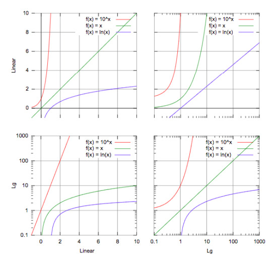
Source: https://courses.lumenlearning.com/boundless-algebra/chapter/graphs-of-exponential-and-logarithmic-functions/
For example, in the third graph, if you have a line similar to the green one, you should consider using logarithms in order to make it linear!
There are lots of things to do so testing all of them is really important.
Conclusion
If you like to play with numbers and advance your data science skill set, learn Python. It is not a very difficult programming language to learn, and the statistics you can generate with it can make a huge difference in your daily work.
Google Analytics, Google Ads, Search Console… Using these tools already offers tons of data, and if you know the concepts of handling data accurately, you will get very valuable insights from them. You can create more accurate traffic forecasts, or analyze Analytics data such as bounce rate, time on page and their relations with the conversion rate. At the end of the day, it might be possible to predict the future of your brand. But these are only a few examples.
If you want to go further in linear regression, check my Google Page Speed Insights OLS model. I’ve built my own dataset and tried to predict the calculation based on speed metrics such as FCP (First Contentful Paint), FMP (First Meaningful Paint) and TTI (Time to Interactive).
In closing, blend your data, try to find correlations and predict your target. Hamlet Batista has a great article about practical data blending. I strongly recommend it before building any regression model.
The post Here’s how I used Python to build a regression model using an e-commerce dataset appeared first on Search Engine Land.
Here’s how I used Python to build a regression model using an e-commerce dataset published first on https://likesandfollowersclub.weebly.com/
0 notes
Text
Programming Linear Regressions
In this post, we want to provide a brief summary of all the necessary steps to create a Linear Regression using the BigML API. As mentioned in our earlier posts, Linear Regression is a supervised learning method to solve regression problems, i.e., the objective field must be numeric.
The API workflow to create a Linear Regression and use it to make predictions is very similar to the one we explained for the Dashboard in our previous post. It’s worth mentioning that any resource created with the API will automatically be created in your Dashboard too so you can take advantage of BigML’s intuitive visualizations at any time.

In case you never used the BigML API before, all requests to manage your resources must use HTTPS and be authenticated using your username and API key to verify your identity. Find below a base URL example to manage Linear Regressions.
https://bigml.io/linearregression?username=$BIGML_USERNAME;api_key=$BIGML_API_KEY
You can find your authentication details in your Dashboard account by clicking in the API Key icon in the top menu.
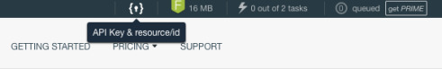
The first step in any BigML workflow using the API is setting up authentication. Once authentication is successfully set up, you can begin executing the rest of this workflow.
export BIGML_USERNAME=nickwilson export BIGML_API_KEY=98ftd66e7f089af7201db795f46d8956b714268a export BIGML_AUTH="username=$BIGML_USERNAME;api_key=$BIGML_API_KEY;"
1. Upload Your Data
You can upload your data in your preferred format, from a local file, a remote file (using a URL) or from your cloud repository e.g., AWS, Azure etc. This will automatically create a source in your BigML account.
First, you need to open up a terminal with curl or any other command-line tool that implements standard HTTPS methods. In the example below, we are creating a source from a local CSV file containing some house data listed in Airbnb, each row representing one house’s information.
curl "https://bigml.io/source?$BIGML_AUTH" -F [email protected]
2. Create a Dataset
After the source is created, you need to build a dataset, which serializes your data and transforms it into a suitable input for the Machine Learning algorithm.
curl "https://bigml.io/dataset?$BIGML_AUTH" -X POST -H 'content-type: application/json' -d '{"source":"source/5c7631694e17272d410007aa"}'
Then, split your recently created dataset into two subsets: one for training the model and another for testing it. It is essential to evaluate your model with data that the model hasn’t seen before. You need to do this in two separate API calls that create two different datasets.
To create the training dataset, you need the original dataset ID and the sample_rate (the proportion of instances to include in the sample) as arguments. In the example below, we are including 80% of the instances in our training dataset. We also set a particular seed argument to ensure that the sampling will be deterministic. This will ensure that the instances selected in the training dataset will never be part of the test dataset created with the same sampling hold out.
curl "https://bigml.io/dataset?$BIGML_AUTH" -X POST -H 'content-type: application/json' -d '{"origin_dataset":"dataset/5c762fcd4e17272d4100072d", "sample_rate":0.8, "seed":"myairbnb"}'
For the testing dataset, you also need the original dataset ID and the sample_rate, but this time we combine it with the out_of_bag argument. The out of bag takes the (1- sample_rate) instances, in this case, 1-0.8=0.2. Using those two arguments along with the same seed used to create the training dataset, we ensure that the training and testing datasets are mutually exclusive.
curl "https://bigml.io/dataset?$BIGML_AUTH" -X POST -H 'content-type: application/json' -d '{"origin_dataset":"dataset/5c762fcd4e17272d4100072d", "sample_rate":0.8, "out_of_bag":true, "seed":"myairbnb"}'
3. Create a Linear Regression
Next, use your training dataset to create a Linear Regression. Remember that the field you want to predict must be numeric. BigML takes the last numerical field in your dataset as the objective field by default unless it is specified. In the example below, we are creating a Linear Regression including an argument to indicate the objective field. To specify the objective field you can either use the field name or the field ID:
curl "https://bigml.io/linearregression?$BIGML_AUTH" -X POST -H 'content-type: application/json' -d '{"dataset":"dataset/68b5627b3c1920186f000325", "objective_field":"price"}'
You can also configure a wide range of the Linear Regression parameters at creation time. Read about all of them in the API documentation.
Usually, Linear Regressions can only handle numeric fields as inputs, but BigML automatically performs a set of transformations such that it can also support categorical, text and items input fields. Keep in mind that BigML uses dummy encoding by default, but you can configure other types of transformations using the different encoding options provided.
4. Evaluate the Linear Regression
Evaluating your Linear Regression is key to measure its predictive performance against unseen data.
You need the linear regression ID and the testing dataset ID as arguments to create an evaluation using the API:
curl "https://bigml.io/evaluation?$BIGML_AUTH" -X POST -H 'content-type: application/json' -d '{"linearregression":"linearregression/5c762c6b4e17272d42000617", "dataset":"dataset/5c762f3a4e17272d41000724"}'
5. Make Predictions
Finally, once you are satisfied with your model’s performance, use your Logistic Regression to make predictions by feeding it new data. Linear Regression in BigML can gracefully handle missing values for your categorical, text or items fields.
In BigML you can make predictions for a single instance or multiple instances (in batch). See below an example for each case.
To predict one new data point, just input the values for the fields used by the Linear Regression to make your prediction. In turn, you get a prediction result for your objective field along with confidence and probability intervals.
curl "https://bigml.io/prediction?$BIGML_AUTH" -X POST -H 'content-type: application/json' -d '{"linearregression":"linearregression/5c762c6b4e17272d42000617", "input_data":{"room":4, "bathroom":2, ...}}'
To make predictions for multiple instances simultaneously, use the Linear Regression ID and the new dataset ID containing the observations you want to predict.
curl "https://bigml.io/batchprediction?$BIGML_AUTH" -X POST -H 'content-type: application/json' -d '{"linearregression":"linearregression/5c762c6b4e17272d42000617", "dataset":"dataset/5c128e694e1727920d00000c", "output_dataset": true}'
If you want to learn more about Linear Regression please visit our release page for documentation on how to use Linear Regression with the BigML Dashboard and the BigML API. In case you still have some questions be sure to reach us at [email protected] anytime!
The Official Blog of BigML.com published first on The Official Blog of BigML.com
0 notes
Text
Regresión Lineal Simple
Sinceramente pensé que aprender mate para ml sería más difícil que interiorizar la lógica de programación, porque dentro de mi mente la lógica usada era muy diferente, pero cuando entendí este tema de la regresión lineal simple me di cuenta de un super secreto a la vista de todos... La lógica matemática es un ancestro de la lógica de programación.
Primero tenía que en averiguar el objetivo de una ecuación usada en un tutorial de yt que estaba viendo.
y = mx + b
Pues no tiene sentido usar una ecuación que no se entiende.
Básicamente se trata de que con una variable x que ponés se puede calcular el valor aproximado de un valor y.
¿Y esto pa qué sirve? Bueno...
Digamos que tenemos estos datos:
Horas que estudió un estudiante -> x: [1,9,6,11,16,18,2,2,5,7]
Las notas respectivas -> y: [27,66,55,90,100,97,24,34,60,70]
Se necesita una fila de x*y y otra x*x
Y por último, las sumatorias
Con estos datos si le doy un número de x horas de estudio a la ecuación esta me devolverá una nota aproximada para las horas que estudié.
Las sumatorias son básicamente una suma de todos los elementos de una columna.
Bueno, ya que se tiene los x y los y se puede hacer algo que se llama diagrama de dispersión(suena muy cool), and guest what, es un plano donde se dispersan los datos, más o menos algo así:

En la ecuación y = mx + b tenía que averiguar qué era m y b.
Así que básicamente lo diré en javascript:
// m = (n * obj._xy - obj._x * obj._y) / (n * obj._xx - Math.pow(obj._x, 2)); // b = (obj._y * obj._xx - obj._x * obj._xy) / (n * obj._xx - Math.pow(obj._x, 2));
Todas las variables, con un guión bajo antes, son sumatorias, y n es la cantidad de datos en el array de x( [1,9,6,11,16,18,2,2,5,7] ), en este caso serían diez.
Ya con todo eso dicho aquí va mi algoritmo de ejemplo:
const xyObj = { x: [1,9,6,11,16,18,2,2,5,7], // x y: [27,66,55,90,100,97,24,34,60,70] // y // xy // x*x } function linearRegression(obj) { function simpleLinearRegression(x){ obj['xy'] = []; obj['xx'] = []; // summation obj['_x'] = 0; obj['_y'] = 0; obj['_xy'] = 0; obj['_xx'] = 0; for (let i = 0; i < obj.x.length; i++) { obj.xy.push(obj.x[i] * obj.y[i]); obj.xx.push(obj.x[i] * obj.x[i]); } for (let i = 0; i < obj.x.length; i++) { obj._x += obj.x[i]; obj._y += obj.y[i]; obj._xy += obj.xy[i]; obj._xx += obj.xx[i]; } let m, b, y; const n = obj.x.length; m = (n * obj._xy - obj._x * obj._y) / (n * obj._xx - Math.pow(obj._x, 2)); b = (obj._y * obj._xx - obj._x * obj._xy) / (n * obj._xx - Math.pow(obj._x, 2));
y = m * x + b; return y; } // scaleX to scale the graphic width // scaleY to scale the graphic height // bool false, 0, undefined... to avoid drawing the line function drawGraphicXY(scaleX = 1,scaleY = 1, bool = true, cWidth = 400, cHeight = 400) { const c = document.querySelector('canvas'); const ctx = c.getContext('2d'); const manageCanvasSize = (function() { c.width = cWidth; c.height = cHeight; window.addEventListener('resize', ()=> { c.width = cWidth; c.height = cHeight; }); })(); let lineToDraw = []; for(let i = 0; i < c.width / scaleX; i++) { let yResult = simpleLinearRegression(i); lineToDraw.push({ y: yResult * scaleY, x: i * scaleX, // use to draw in canvas realX: i, realY: yResult }); // console.log(i, '-', yResult); } // console.log(lineToDraw); function drawLine() { ctx.beginPath(); ctx.fillStyle = '#FF0000'; for(let i of lineToDraw) { ctx.fillRect(i.x,c.height - i.y,5,5); } } function drawXYDots() { ctx.fillStyle = '#210CE8'; ctx.beginPath(); for (let i = 0; i < obj.x.length; i++) { //ctx.fillRect(obj.x[i] * scaleX - scaleDotX / 2, // c.height - obj.y[i] * scaleY - scaleDotY / 2, // scaleDotX, scaleDotY); ctx.fillText(`${i+1}°(${obj.x[i]},${obj.y[i]})`, obj.x[i] * scaleX, c.height - obj.y[i] * scaleY); ctx.font = '12px sans-serif'; } } function animate() { ctx.clearRect(0, 0, c.width, c.height); drawXYDots(obj, ctx); if(bool) drawLine(); window.requestAnimationFrame(animate); }; animate(); } // simpleLinearRegression(obj, 10); return { slr: simpleLinearRegression, dxy: drawGraphicXY } }
let studentsGrades = linearRegression(xyObj); console.log(studentsGrades.slr(11.2)); studentsGrades.dxy(18, 3.5);
Al final la función studentsGrades.dxy(18, 3.5), si se tiene un canvas en html producirá este gráfico:
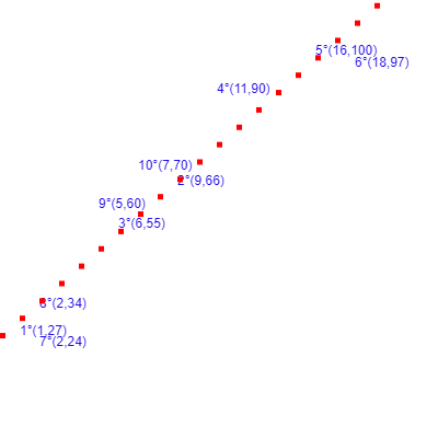
Y entonces solo quería decir que entendí esto de la regresión linear simple. Cool.
0 notes
Text
Homework 1 Solution
Note:
You are expected to submit both a report and code. For your code, please include clear README files. When not specifically mentioned, use the default data provided in our program package.
“########## Please Fill Missing Lines Here ##########” is used where input from you is needed.
1. Linear Regression
In LinearRegression\linearRegression.py, fill in the missing lines in the python code…
View On WordPress
0 notes
Text
Machine Learning with Scikit-Learn in Python

To create a simple machine learning model in Python, you can use the scikit-learn library to train a Linear Regression Model. Below is a step-by-step guide to create a simple machine learning model in Python using only 5 lines of code.
EXPLORING SIMPLE EXEMPLE.
Step 1: Install scikit-learn
```python
pip install scikit-learn
```
Step 2: Sample Training Set
```python
X = [[1, 2, 3], [2, 3, 4], [3, 4, 5]] # Input
y = [14, 20, 26] # Output
```
Step 3: Create and Train the Model
```python
from sklearn.linear_model import LinearRegression
model = LinearRegression()
model.fit(X, y)
```
Step 4: Test the Model
```python
test_data = [[4, 5, 6]] # Test input
predicted_output = model.predict(test_data)
print(predicted_output) # Expected output: [32]
```
In this example, we are using a simple linear regression model to predict an output based on the input features. The model is trained using the input-output pairs, and then tested with new input data to make predictions.

EXPLORING ALTERNATIVES
Machine Learning with Scikit-Learn in Python:
Machine learning (ML) empowers computers to learn from data without explicit programming. Scikit-learn is a popular Python library that streamlines ML tasks. Here's a step-by-step approach to building a simple linear regression model using scikit-learn:
1. Installation:
pip install scikit-learn
2. Sample Training Set:
# Input data (features)
X = [[1, 2, 3], [2, 3, 4], [3, 4, 5]]
# Output data (target)
y = [14, 20, 26]
Explanation:
X represents the features or independent variables that the model will learn from. In this example, it's a 3x3 array where each row represents a data point with three features.
represents the target variable or the value the model aims to predict. Here, it's a list containing the corresponding outputs for each data point in X.

3. Create and Train the Model:
from sklearn.linear_model import LinearRegression
model = LinearRegression()
model.fit(X, y)
Explanation:
We import the LinearRegression class from scikit-learn's linear_model module.
We create an instance of the LinearRegression class, essentially initializing a linear regression model.
The model.fit(X, y) method trains the model using the input features (X) and the corresponding target values (y). During training, the model learns the underlying linear relationship between the features and the target variable.
4. Test the Model:
test_data = [[4, 5, 6]] # New data point for prediction
predicted_output = model.predict(test_data)
print(predicted_output) # Expected output: [32]
Explanation:
We create a new data point test_data with features similar to those in the training set.
The model.predict(test_data) method uses the trained model to predict the target value for the new data point. Here, it predicts an output of approximately 32 based on the learned linear relationship.
Practical Examples:
Real Estate Price Prediction:
Features: House size (sq ft), number of bedrooms, location
Target variable: Selling price
Stock Price Prediction:
Features: Past closing prices, trading volume, market trends
Target variable: Future closing price
AI Solutions for the Market
Recommender Systems: Recommend products, movies, or music based on user preferences (e.g., Netflix, Amazon).
Fraud Detection: Analyze transactions to identify fraudulent activities (e.g., credit card companies, banks).
Customer Service Chatbots: Provide automated customer support and answer frequently asked questions.
Machine Learning for Enterprises
Corporations can leverage ML for various tasks:
Demand Forecasting: Predict future customer demand to optimize inventory management and production planning.
Targeted Marketing: Personalize marketing campaigns to reach specific customer segments with high-impact messaging.
Product Design: Analyze customer feedback and usage data to improve product design and functionality.
Expanding the Linear Regression Algorithm
Linear regression is a versatile foundation for various ML tasks. Here's how it can be extended:
Polynomial Regression: Capture non-linear relationships between features and target variables by introducing polynomial terms.
Logistic Regression: Model binary classification problems (e.g., spam detection, credit risk assessment).
Regularization: Techniques like L1 or L2 regularization can prevent overfitting and improve modelgeneralizability.
Understanding the Code Snippet
from sklearn.linear_model import LinearRegression
model = LinearRegression()
model.fit(X, y)
predicted_output = model.predict(test_data)
This code imports the LinearRegression class, creates a model instance, trains it using sample data (X, y), and generates a prediction for new data (test_data).
I hope this comprehensive explanation empowers you to create and apply ML models effectively.
MORE EXEMPLES
Here are two Python code snippets demonstrating different machine learning concepts:
1. Linear Regression for Price Prediction:
# Import libraries
from sklearn.linear_model import LinearRegression
# Sample data (features and target variable)
X = [[1500, 3], [2000, 4], [2500, 5]] # House size (sq ft), number of bedrooms
y = [300000, 400000, 500000] # Price
# Create and train the model
model = LinearRegression()
model.fit(X, y)
# New data for prediction
test_data = [[3000, 4]]
# Predict the price
predicted_price = model.predict(test_data)
print("Predicted price:", predicted_price[0])
This code implements a linear regression model to predict house prices based on size and number of bedrooms.
2. K-Nearest Neighbors for Classification:
# Import libraries
from sklearn.neighbors import KNeighborsClassifier
# Sample data (features and target labels)
X = [[1, 2], [3, 4], [5, 6], [7, 8], [1, 4], [3, 2]] # Features
y = ["red", "red", "blue", "blue", "red", "red"] # Class labels (red or blue)
# Create and train the model
knn = KNeighborsClassifier(n_neighbors=3) # 3 nearest neighbors
knn.fit(X, y)
# New data for prediction
test_data = [[6, 9]]
# Predict the class label
predicted_label = knn.predict(test_data)
print("Predicted class:", predicted_label[0])
This code uses a K-Nearest Neighbors (KNN) classifier to categorize data points (red or blue) based on their proximity to labeled examples in the training data.
Here's a breakdown of the two machine learning concepts explored in the Python code snippets:
1. Linear Regression:
Concept: It's a statistical approach for modeling the relationship between a dependent variable (what you want to predict) and one or more independent variables (what you're basing your prediction on). The resulting model is a linear equation that approximates the underlying trend in the data.
Example: In the code, linear regression predicts house prices (dependent variable) based on house size and number of bedrooms (independent variables). The model learns the linear relationship between these features and prices from the training data and uses that knowledge to estimate prices for new houses.
2. K-Nearest Neighbors (KNN):
Concept: A non-parametric classification algorithm that classifies data points based on their similarity to labeled data points in the training set. It finds the k nearest neighbors (data points most similar) to the new data point and assigns the majority class label from those neighbors.
Example: The code employs KNN to classify data points as "red" or "blue." For a new data point, KNN identifies the 3 closest labeled points (k=3) from the training data. If the majority of those 3 points are classified as "red," the new data point is also predicted as "red."
These are just two fundamental ML algorithms, but they represent different approaches to learning from data. Linear regression excels at modeling continuous relationships, while KNN is well-suited for classification tasks.

RDIDINI PROMPT ENGINEER
0 notes
Text
Homework 1 Solution
Note:
You are expected to submit both a report and code. For your code, please include clear README files. When not specifically mentioned, use the default data provided in our program package.
“########## Please Fill Missing Lines Here ##########” is used where input from you is needed.
1. Linear Regression
In LinearRegression\linearRegression.py, fill in the missing lines in the python code…
View On WordPress
0 notes
Text
How to Make Predictions with scikit-learn
How to anticipate category or regression outcomes with scikit-learn models in Python.
Once you select and fit a last device discovering model in scikit-learn, you can use it to make predictions on new information instances.
There is some confusion among novices about how precisely to do this. I often see concerns such as:
How do I make predictions with my model in scikit-learn?
In this tutorial, you will discover precisely how you can make category and regression forecasts with a settled maker discovering model in the scikit-learn Python library.
After completing this tutorial, you will understand:
Let's get started.
Gentle Introduction to Vector Standards in Device Knowing Photo by Cosimo, some rights reserved.Tutorial Introduction This tutorial is divided into 3
parts; they are: 1. First Finalize Your Design Prior to you can
make forecasts, you must train
a final model. You might have trained models using k-fold cross validation or train/test splits of your data. This was carried out in order to give you a price quote of the skill of the design on out-of-sample data, e.g. new information. These models have served their function and can now be disposed of.
You now need to train a last model on all of your available information.
You can find out more about how to train a last design here: 2.
How to Predict With Classification Designs Classification issues
are those where the model finds out a mapping in between input functions and an output function that is a label, such as "spam "and"not spam."Below is sample code of a settled LogisticRegression design for a basic binary classification problem. Although we are utilizing LogisticRegression in this tutorial, the very same functions are offered on almost all category
algorithms in scikit-learn. from sklearn. linear_model import LogisticRegression After completing your design, you might want to conserve the design to file, e.g. via pickle. When saved, you can load the design any time and use it to makeforecasts. For an example of this, see the post: For simplicity, we will avoid this action for the examples in this tutorial. There are
2 kinds of category forecasts we might wish to make with our settled model; they are class predictions and possibility forecasts. Class Predictions A class forecast is:
provided the finalized model and several information circumstances, forecast the class for the data circumstances. We do not understand the outcome classes for the brand-new information. That is why we need the model in the very first place. We can predict the class for brand-new information circumstances using our settled category
model in scikit-learn utilizing the anticipate() function. We have one or more information instances in an array called Xnew. This can be passed to the predict() function on our design in order to anticipate the class worths for each circumstances in the variety. Multiple Class Predictions Let's make this concrete with an example of forecasting several data instances simultaneously.
from sklearn. linear_model import LogisticRegression
for i in range(len(Xnew)): print("X=%s, Predicted =%s"%
(Xnew [ i], ynew [i].))Running the example anticipates the class for the three new information instances, then
prints the information and the forecasts together.X=[crayon-sy">.-0.79415228 2.10495117], Forecasted=0
X=[crayon-sy">.-8.25290074 -4.71455545], Predicted=1 X =[. -2.18773166 3.33352125], Anticipated=0 Single Class Prediction If you had simply one brand-new information instance, you can supply this as circumstances wrappedin a range to
the predict( )function; for instance:< div class ="crayon-line crayon-striped-line "id ="crayon-5c531b1e48f05240900963-2"> from sklearn. linear_model import LogisticRegression Running the example prints the single instance and the forecasted class. X= [-0.79415228, 2.10495117], Anticipated=0
A Note on Class Labels When you prepared your information, you will have
mapped the class values from your
domain (such as strings)to integer worths. You may have used a< a href ="http://scikit-learn.org/stable/modules/generated/sklearn.preprocessing.LabelEncoder.html#sklearn.preprocessing.LabelEncoder"> LabelEncoder. This LabelEncodercan be utilized to convert the integers back into string values by means of the inverse_transform()function. For this factor, youmay want to save(pickle)the LabelEncoder utilized to encode your y values when fitting your last model. Probability Predictions
Another type of forecast you might want to make is the possibility of the data
circumstances belonging to each class
. This is called a possibility forecast where provided a new circumstances, the model returns the likelihood for each result class as a value between 0 and 1.
You can make these types of predictions in scikit-learn by calling the predict_proba ()function, for instance : ynew=model. predict_proba( Xnew)This function is only readily available on those classification models capable of making a likelihood forecast, which is most, but not all, models. The example listed below makes a likelihood prediction for each example in the Xnew range of data
instance. from sklearn. linear_model import LogisticRegression # make a prediction for i in range(len(Xnew)): print("X=%s, Forecasted=%s"%(Xnew [i]., ynew [i]
)Running the circumstances makes the probability predictions and after that prints the input information circumstances and the probability of each circumstances belonging to the first and 2nd classes( 0 and 1). X=[
-0.79415228 2.10495117], Predicted=[ 0.94556472 0.05443528] X=[ -8.25290074 -4.71455545], Forecasted=[ 3.60980873e-04 9.99639019e-01] X=[crayon-sy">.-2.18773166 3.33352125], Predicted=[crayon-sy">.0.98437415 0.01562585] This can be handy in your application if you want to present the probabilities to the userfor expert interpretation. 3. How to Anticipate With Regression Designs Regression is a supervised learning problem where, provided input examples, the design finds out a mapping to suitable output amounts, such as"0.1"and"0.2", and so on. Below is an example of a finalized LinearRegression design. Again, the functions showed for making regression forecastsapply to all of the regression models available in scikit-learn. from sklearn. linear_model import LinearRegression from sklearn. datasets import make_regression We can forecast quantities with the finalized regression design by calling the anticipate()function on the finalized design. As with classification, the forecast ()function takes a list or array of several data instances. Numerous Regression Forecasts The example listed below demonstrates how to make regression predictions on several data instances with an unknown anticipated outcome. from sklearn. linear_model import LinearRegression from sklearn. datasets import make_regression for i in range(len(Xnew))
:< div class="crayon-line"id="crayon-5c531b1e48f68804316190-15" > print("X= %s, Predicted=%s" %(Xnew [i], ynew [i])Running the example makes numerous forecasts, then
prints the inputs and forecasts side-by-side for evaluation. X=[ -1.07296862 -0.52817175], Forecasted =-61.32459258381131X=[crayon-v">. -0.61175641 1.62434536], Forecasted=-30.922508147981667
X=[crayon-v">. -2.3015387 0.86540763], Predicted=-127.34448527071137 Single Regression Prediction The exact same function can be used to make a forecast for a single information instance as long as it is appropriately covered in a surrounding list or array.
from sklearn.
linear_model import LinearRegression from sklearn. datasets import make_regression< div class ="crayon-line crayon-striped-line"id="crayon-5c531b1e48f6c704504705-10"> Xnew=[ [-1.07296862,-0.52817175]] # show the inputsand forecasted outputsprint("X=%s, Forecasted=%s"%(Xnew [0], ynew [0])Running
the example makes a single forecast and prints the information instance and prediction for evaluation. X=[ -1.07296862, -0.52817175]crayon-sy">,Forecasted=-77.17947088762787 Additional
Reading In this tutorial, you discovered how you canmake classification and regression predictions with a completed machine discovering model in the scikit-learn Python library. Specifically, you learned: Do youhave any questions ? Ask your questions in the comments listed below and I will do my best to answer. Frustrated With Python Maker Learning? Establish Your Own Models in Minutes ... with just a couple of lines of scikit-learn code Discover how in my brand-new Ebook: Device Knowing Proficiency With Python Covers self-study tutorials and end-to-end tasks like: Packing information, visualization, modeling, tuning, and much more ... Lastly Bring Machine Knowing To Your Own Projects Skip the Academics. Simply Results.
0 notes
Text
Multiple Regression using Python
# Multiple Linear Regression
# Importing the libraries import numpy as np import matplotlib.pyplot as plt import pandas as pd import seaborn as sns from statsmodels.formula.api import ols import matplotlib.pyplot as plt import pylab import scipy.stats as stats import statsmodels.api as sm import statsmodels.formula.api as smf # Importing the dataset dataset = pd.read_csv('C:/Users/Janani/Desktop/50_Startups.csv') dataset.columns = ('RDSpend','Administration','MarketingSpend','State','Profit')
X = dataset.iloc[:, :-1].values y = dataset.iloc[:, 4].values # Encoding categorical data from sklearn.preprocessing import LabelEncoder, OneHotEncoder labelencoder = LabelEncoder() X[:, 3] = labelencoder.fit_transform(X[:, 3]) onehotencoder = OneHotEncoder(categorical_features = [3]) X = onehotencoder.fit_transform(X).toarray() # Avoiding the Dummy Variable Trap X = X[:, 1:] # Splitting the dataset into the Training set and Test set from sklearn.cross_validation import train_test_split X_train, X_test, y_train, y_test = train_test_split(X, y, test_size = 0.2, random_state = 0) # Fitting Multiple Linear Regression to the Training set from sklearn.linear_model import LinearRegression regressor = LinearRegression() regressor.fit(X_train, y_train) # Predicting the Test set results y_pred = regressor.predict(X_test)
stats.probplot(y_pred, dist='norm', plot=pylab) pylab.show()
model = smf.ols(formula='Profit ~ RDSpend + Administration + MarketingSpend + State' , data=dataset).fit()
model.summary()
OLS Regression Results ============================================================================== Dep. Variable: Profit R-squared: 0.951 Model: OLS Adj. R-squared: 0.945 Method: Least Squares F-statistic: 169.9 Date: Sun, 11 Nov 2018 Prob (F-statistic): 1.34e-27 Time: 23:00:19 Log-Likelihood: -525.38 No. Observations: 50 AIC: 1063. Df Residuals: 44 BIC: 1074. Df Model: 5 Covariance Type: nonrobust ===================================================================================== coef std err t P>|t| [0.025 0.975] ------------------------------------------------------------------------------------- Intercept 5.013e+04 6884.820 7.281 0.000 3.62e+04 6.4e+04 State[T.Florida] 198.7888 3371.007 0.059 0.953 -6595.030 6992.607 State[T.New York] -41.8870 3256.039 -0.013 �� 0.990 -6604.003 6520.229 RDSpend 0.8060 0.046 17.369 0.000 0.712 0.900 Administration -0.0270 0.052 -0.517 0.608 -0.132 0.078 MarketingSpend 0.0270 0.017 1.574 0.123 -0.008 0.062 ============================================================================== Omnibus: 14.782 Durbin-Watson: 1.283 Prob(Omnibus): 0.001 Jarque-Bera (JB): 21.266 Skew: -0.948 Prob(JB): 2.41e-05 Kurtosis: 5.572 Cond. No. 1.45e+06 ==============================================================================
model_fitted_y = model.fittedvalues plt.hist(model_fitted_y.pearson_resid) model_residuals = model.resid model_norm_residuals = model.get_influence().resid_studentized_internal model_norm_residuals_abs_sqrt = np.sqrt(np.abs(model_norm_residuals)) model_abs_resid = np.abs(model_residuals)
model_leverage = model.get_influence().hat_matrix_diag model_cooks = model.get_influence().cooks_distance[0] stats.probplot(model, dist="norm", plot=pylab) pylab.show()
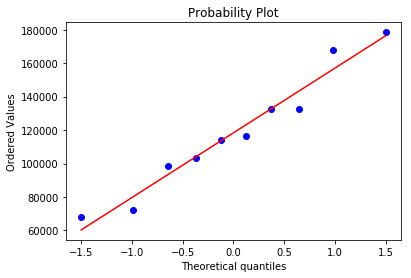
#Q-Q plot for normality fig4=sm.qqplot(model.resid, line='r')

The qq-plot clearly displays the points lie along the line and it clearly indicates there are no skewness. There are no outliers.
fig, ax = plt.subplots(figsize=(12,8)) fig = sm.graphics.influence_plot(model, ax=ax, criterion="cooks")
Influence Leverage Plot:
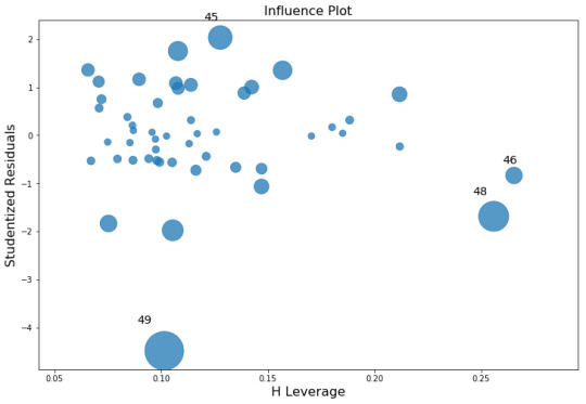
There are only three outliers hence there are not many influencers to skew the data.
# simple plot of residuals
stdres=pd.DataFrame(model.resid_pearson) plt.plot(stdres, 'o', ls='None') l = plt.axhline(y=0, color='r') plt.ylabel('Standardized Residual') plt.xlabel('Observation Number')

After adjusting for potential confounding factors R&D Spend, Administration, Marketing, State), Profit significantly increased.
0 notes