#mini-batch gradient descent

[machinelearningsite]

Choosing the Right Gradient Descent: Batch vs Stochastic vs Mini-Batch Explained

The blog shows key differences between Batch, Stochastic, and Mini-Batch Gradient Descent. Discover how these optimization techniques impact ML model training.

In my previous post on gradient descent, I explained briefly what gradient descent means and what mathematical idea it holds. A basic gradient descent algorithm involves calculating derivatives of the cost function with respect to the parameters to be optimized. This derivative is calculated over the entire training set as a whole. Now if the data has samples in hundreds of thousands, the…

[xsanghv4]

🔥 TĂNG TỐC HUẤN LUYỆN MÔ HÌNH AI BẰNG PHƯƠNG PHÁP GRADIENT DESCENT! 🚀

Bạn đã từng cảm thấy "quá tải" khi huấn luyện mô hình AI của mình chưa? 🤯 Đừng lo, vì Gradient Descent chính là chìa khóa vàng 🗝️ để bạn tối ưu hóa tốc độ và hiệu quả! ✅

💡 Gradient Descent là gì? Gradient Descent là một thuật toán học máy "quốc dân" 🌍, giúp mô hình của bạn dần tìm ra điểm tối ưu 🎯 để giảm thiểu lỗi và tăng độ chính xác. Nhưng bạn có biết rằng có nhiều biến thể thông minh như Mini-batch, Stochastic Gradient Descent (SGD) hay Momentum có thể thúc đẩy tốc độ hơn nữa? 🚀

🔍 Tại sao nên quan tâm?

Tiết kiệm thời gian ��

Hiệu quả vượt trội 💪

Ứng dụng linh hoạt: Từ học sâu (Deep Learning) 🧠 đến mạng nơ-ron nhân tạo, Gradient Descent đều có thể giúp bạn! 🌟

📖 Tìm hiểu thêm về các mẹo tăng tốc huấn luyện và những case study thực tế ngay tại bài viết chi tiết trên website của chúng tôi! 👉 Tăng tốc huấn luyện mô hình với phương pháp Gradient Descent

Khám phá thêm những bài viết giá trị tại aicandy.vn

[careerguide1]

Optimization Techniques in Machine Learning Training

Optimization techniques are central to machine learning as they help in finding the best parameters for a model by minimizing or maximizing a function. They guide the training process by improving model accuracy and reducing errors.

Common Optimization Algorithms:

Gradient Descent: A widely used algorithm that minimizes the loss function by iteratively moving towards the minimum. Variants include:

Batch Gradient Descent

Stochastic Gradient Descent (SGD)

Mini-batch Gradient Descent

Adam (Adaptive Moment Estimation): Combines the advantages of both AdaGrad and RMSProp.

AdaGrad: Particularly good for sparse data, adjusts the learning rate for each parameter.

RMSProp: Used to deal with the problem of decaying learning rates in gradient descent.

Challenges in Optimization:

Learning Rate: A critical hyperparameter that determines how big each update step is. Too high, and you may overshoot; too low, and learning is slow.

Overfitting and Underfitting: Ensuring that the model generalizes well and doesn’t memorize the training data.

Convergence Issues: Some algorithms may converge too slowly or get stuck in local minima.

Real-World Application in Training:

Practical Exposure: A hands-on course in Pune would likely offer real-world projects where students apply these optimization techniques to datasets.

Project-Based Learning: Students might get to work on tasks like tuning hyperparameters, selecting the best optimization methods for a particular problem, and improving model performance on various data types (e.g., structured data, images, or text).

Career Advancement

The training can enhance skills in AI and ML, making participants capable of optimizing models efficiently. Whether it’s for a career in data science, AI, or machine learning in in Pune, optimization techniques play a vital role in delivering high-performance models.

Would you like to focus on any specific aspects of the training? For example, are you interested in a particular optimization algorithm, or do you want to delve into the practical application through projects in Pune?

[teguhteja]

Mini-Batch Gradient Descent: Optimizing Machine Learning Models

#MachineLearning #MBGD Discover how Mini-Batch Gradient Descent revolutionizes model training! Learn to implement MBGD in Python, optimize your algorithms, and boost performance. Perfect for data scientists and ML engineers looking to level up their skill

Mini-Batch Gradient Descent (MBGD) is a powerful optimization technique that revolutionizes machine learning model training. By combining the best features of Stochastic Gradient Descent (SGD) and Batch Gradient Descent, MBGD offers a balanced approach to model optimization. In this blog post, we’ll explore how MBGD works, its advantages, and how to implement it in Python. Understanding the Need…

[ingoampt]

Day 8 _ Gradient Decent Types : Batch, Stochastic and Mini-Batch

Understanding Gradient Descent: Batch, Stochastic, and Mini-Batch Understanding Gradient Descent: Batch, Stochastic, and Mini-Batch Learn the key differences between Batch Gradient Descent, Stochastic Gradient Descent, and Mini-Batch Gradient Descent, and how to apply them in your machine learning models. Batch Gradient Descent Batch Gradient Descent calculates the gradient of the cost function…

[codeshive]

DD2424 - Assignment 2 solved

In this assignment you will train and test a two layer network with multiple outputs to classify images from the CIFAR-10 dataset. You will train the network using mini-batch gradient descent applied to a cost function that computes the cross-entropy loss of the classifier applied to the labelled training data and an L2 regularization term on the weight matrix. The overall structure of your code…

[codingprolab]

DD2424 - Assignment 2

In this assignment you will train and test a two layer network with multiple outputs to classify images from the CIFAR-10 dataset. You will train the network using mini-batch gradient descent applied to a cost function that computes the cross-entropy loss of the classifier applied to the labelled training data and an L2 regularization term on the weight matrix. The overall structure of your code…

[ardhra2000]

Stochastic Gradient Descent

In the context of machine learning, stochastic gradient descent is a preferred approach for training various models due to its efficiency and relatively low computational cost.

SGD, by updating parameters on a per-sample basis, performs notably faster than batch gradient descent, which calculates the gradient using the whole dataset.

Researchers investigating AIalgorithms utilize SGD as a pivotal step in the development and refining of complex models.

Software developers building Machine Learning applications with large datasets harness SGD's power to ensure effective and efficient model training.

The learning rate is a critical hyperparameter that controls the step size during the optimization process. Setting it too high can cause the algorithm to oscillate and diverge; too low can result in slow convergence. It might initially be large, to make quick progress, but gradually decreased to allow more fine-grained parameter updates to reach the optimal solution.

As deep learning techniques continue to develop and gain complexity, SGD and its variants will remain foundational to training these models.

Reinforcement learning, a rapidly evolving field in artificial intelligence, often involves optimization methods including SGD.

Mini-Batch Gradient Descent, a variation of SGD, combines the advantages of both SGD and Batch Gradient Descent. It updates parameters using a mini-batch of ‘n’ training examples, striking a balance between computational efficiency and convergence stability.

[lutoogyan]

Understanding Gradient Descent for Machine Learning | by Idil Ismiguzel

Newsletter Sed ut perspiciatis unde. Subscribe A deep dive into Batch, Stochastic, and Mini-Batch Gradient Descent algorithms using Python Photo by Lucas Clara on Unsplash Gradient descent is a popular optimization algorithm that is used in machine learning and deep learning models such as linear regression, logistic regression, and neural networks. It uses first-order derivatives iteratively…

[jacob-cs]

Machine Learning by Andrew Ng week 10 ( Summary )

https://www.coursera.org/learn/machine-learning/lecture/CipHf/learning-with-large-datasets

Learning With Large Datasets

위그림의 좌하단의 그림은 high variance 된 알고리즘이며 이런 경우 더 ���은 데이터가 알고리즘 개선에 도움이 된다. 오른쪽의 경우는 high biase 된 경우이며 이런경우는 더이상의 데이터가 도움이 되지 않는다. 

자세한 내용은 week 6 강의를 참조한다. 

https://www.coursera.org/learn/machine-learning/lecture/DoRHJ/stochastic-gradient-descent

Stochastic Gradient Descent

이제까지 사용했던 일반 gradient descent ( batch gradient descent )에 대한 그림이다. 데이터의 양이 엄청 많아지면 ( m의 크기가 커짐) 작은 gradient descent step하나 지나가는데에 엄청난수의 데이터 총합을 매번 구해야 한다. 이렇게 되면 성능에 문제가 생긴다. 그래서 임의의 데이터 하나당 한번의 gradient descent step을 밟는 stochastic gradient descent 방법을 택한다. stochastic gradient descent는 꼭 linear regression아니더라도 다양한 알고리즘과 함께 사용 가능하다. 

빨간색은 일반 gradient descent 궤적이다.

보라색은 stochastic gradient descent 궤적이다. 결과적으로 local minimum에 도착할수도 있고 아닐수도 있지만 근처에 도착하는 것은 맞다. for loop를 감싸는 repeat은 보통 1-10정도 수행한다. 다만 엄청난 수의 데이터가 있는 경우 1번에도 좋은 결과는 만들어낸다.

https://www.coursera.org/learn/machine-learning/lecture/9zJUs/mini-batch-gradient-descent

Mini-Batch Gradient Descent

일반 batch gradient는 모든 데이터값에대한 cost의 총합을 구하고 이에 대한 partial derivative 를 통해 기울기를 구하고 이에 learning rate을 구해서 새로운 theta를 구하는 과정을 거친다. 데이터의 수가 많아지면 성능에 문제가 생기므로 무작위 데이터 하나를 가져와 그에 대한 cost를 이용하는 stocastic gradient descent 방법을 이용할수 있다. 또 몇몇 데이터를 이용하는 mini batch gradient descent를 이용할수도 있다. 좋은 선형대수 라이브러리의 경우 vectorization을 이용한 작업에 병렬연산을 제공하므로 하나의 데이터를 이용하는 것이나 여러데이터를 이용하는 것이나 큰차이가 없다. 

https://www.coursera.org/learn/machine-learning/lecture/fKi0M/stochastic-gradient-descent-convergence

Stochastic Gradient Descent Convergence

Stochastic Gradient descent 가 잘 작동하는지 ( cost 가 점점 감소하는지) 확인 하는 작업을 설명한다. 일정 수의 데이터 cost결과를 중간 중간 확인하는 방식으로 한다. 이 강의에서는 1000개의 데이터를 사용하고 있다. 

위위 그림에서 말하던 확인(plot) 결과를 보여주는 그래프이다. 좌상단의 그림의 경우 파란 그래프는 빨간 그래프보다 큰 알파값을 사용했으며 점차 cost가 줄어드는 것을 알수 있다. 

우상단의 경우 빨간 그래프는 파란 그래프보다 큰 숫자의 데이터를 이용 cost를 측정한 경우이다. 그래프가 부드럽게 바뀐것을 볼수 있으며 cost는 점차 줄고 있다.

좌하단 파란 그래프의 경우 cost가 전반적으로 줄고 있는지 알수 없다. 이런 경우 보다 많은 수의 데이터를 이용 보라색, 빨간색 그래프처럼 결과가 나오게 수정한다. 이렇게 바꾸면 미세하게 줄거나 늘고 있는 것을 볼수 있다. 

우하단의 그래프는 cost가 점차 상승하고 있으며 이런 경우 작은 값의 알파를 사용해 본다.

점차 minimum에 접근하다가 minimum근처를 배회하는 것을 위그림에서 볼수있다. 이를 보완하기 위한 작업을 아래그림에서 설명한다. 

두 상수를 이용해서 점차 learning rate값을 작게 만들어서 조금더 minimum에 다가가고 그곳에 머물게 하는 방법이다.

https://www.coursera.org/learn/machine-learning/lecture/ABO2q/online-learning

online learning

저장된 data 이용하기 보다 끊임없이 제공되는 데이터를 이용할수 있는 경우 사용하는 방법으로 데이터는 한번 사용하고 버린다. 그래서 그림 하단 알고리즘을 보면 x i , y i 가 ���닌 x y를 사용한다. 이런 경우 사용자의 preferece 변화에 신속하게 대응할수 있다.

위와 같은 영역에서 사용될수 있다. 순간적으로 발생하는 데이터에 반응하는 경우에 online learning 를 사용할수 있다.

https://www.coursera.org/learn/machine-learning/lecture/10sqI/map-reduce-and-data-parallelism

Map Reduce and Data Parallelism

대용량의 데이터를 처리해야 하는 경우 이를 여러부분으로 나누어 처리하는 방법을 이용할수 있다. map- reduce, data parallelism을 이용할수 있다.

theta j에서 j는 feature이다. n은 feature의 총갯수.

위 그림은 여러 컴퓨터를 이용한 병렬 처리를 보여주고 있다.

한 컴퓨터내의 여러 코어를 이용한 병렬 처리를 보여주고 있다.

때로는 라이브러이에서 기본적으로 병렬처리를 제공하는 경우도 있다. 선형대수 처리를 하는 경우 병렬처리를 제공하는 경우도 있다.

[leedsomics]

Optimal transport-based machine learning to match specific patterns: application to the detection of molecular regulation patterns in omics data. (arXiv:2107.11192v3 [q-bio.GN] UPDATED)

We present several algorithms designed to learn a pattern of correspondence between two data sets in situations where it is desirable to match elements that exhibit a relationship belonging to a known parametric model. In the motivating case study, the challenge is to better understand micro-RNA regulation in the striatum of Huntington's disease model mice. The algorithms unfold in two stages. First, an optimal transport plan P and an optimal affine transformation are learned, using the Sinkhorn-Knopp algorithm and a mini-batch gradient descent. Second, P is exploited to derive either several co-clusters or several sets of matched elements. A simulation study illustrates how the algorithms work and perform. The real data application further illustrates their applicability and interest. http://dlvr.it/SkHxsR

[craigbrownphd]

If you did not already know

Stochastic Stratified Average Gradient (SSAG) SGD (Stochastic Gradient Descent) is a popular algorithm for large scale optimization problems due to its low iterative cost. However, SGD can not achieve linear convergence rate as FGD (Full Gradient Descent) because of the inherent gradient variance. To attack the problem, mini-batch SGD was proposed to get a trade-off in terms of convergence rate and iteration cost. In this paper, a general CVI (Convergence-Variance Inequality) equation is presented to state formally the interaction of convergence rate and gradient variance. Then a novel algorithm named SSAG (Stochastic Stratified Average Gradient) is introduced to reduce gradient variance based on two techniques, stratified sampling and averaging over iterations that is a key idea in SAG (Stochastic Average Gradient). Furthermore, SSAG can achieve linear convergence rate of $\mathcal {O}((1-\frac{\mu}{8CL})^k)$ at smaller storage and iterative costs, where $C\geq 2$ is the category number of training data. This convergence rate depends mainly on the variance between classes, but not on the variance within the classes. In the case of $C\ll N$ ($N$ is the training data size), SSAG’s convergence rate is much better than SAG’s convergence rate of $\mathcal {O}((1-\frac{\mu}{8NL})^k)$. Our experimental results show SSAG outperforms SAG and many other algorithms. … BitSplit-Net Significant computational cost and memory requirements for deep neural networks (DNNs) make it difficult to utilize DNNs in resource-constrained environments. Binary neural network (BNN), which uses binary weights and binary activations, has been gaining interests for its hardware-friendly characteristics and minimal resource requirement. However, BNN usually suffers from accuracy degradation. In this paper, we introduce ‘BitSplit-Net’, a neural network which maintains the hardware-friendly characteristics of BNN while improving accuracy by using multi-bit precision. In BitSplit-Net, each bit of multi-bit activations propagates independently throughout the network before being merged at the end of the network. Thus, each bit path of the BitSplit-Net resembles BNN and hardware friendly features of BNN, such as bitwise binary activation function, are preserved in our scheme. We demonstrate that the BitSplit version of LeNet-5, VGG-9, AlexNet, and ResNet-18 can be trained to have similar classification accuracy at a lower computational cost compared to conventional multi-bit networks with low bit precision ( https://analytixon.com/2022/12/02/if-you-did-not-already-know-1900/?utm_source=dlvr.it&utm_medium=tumblr

[towardsai]

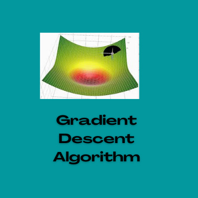
Gradient Descent for Machine Learning (ML) 101 with Python Tutorial Author(s): Towards AI Team A three-dimensional wireframe plot of the unnormalized sin(x) function. | Source: Creative Commons by Wikimedia [1] A tutorial diving into the gradient descent algorithm for machine learning (ML) with Python Author(s): Saniya Parveez, Roberto Iriondo This tutorial’s code is available on Github and its full implementation as well on Google Colab. Table of Contents What is Gradient Descent? Cost function Gradients Python Implementation Learning Rate Convergence Convex Function Batch Gradient Descent Stochastic Gradient Descent Mini-Batch Gradient Descent Conclusion Resources References #MachineLearning #ML #ArtificialIntelligence #AI #DataScience #DeepLearning #Technology #Programming #News #Research #MLOps #EnterpriseAI #TowardsAI #Coding #Programming #Dev #SoftwareEngineering https://bit.ly/3j8lE4H #programming #datascience #editorial

[mk6076225]

Why do we want better optimization algorithms?

To instruct a neural network, we want to outline a loss feature to measure the distinction between the network’s predictions and the ground reality label. During training, we seem to be for a precise set of weight parameters that the neural community can use to make an correct prediction. This concurrently leads to a decrease cost of the loss function.

Gradient Descent:

 From the title we might also without problems get the idea, a descent in the gradient of the loss feature is acknowledged gradient descent. Simply, gradient descent is the approach to locate a valley (comparable to minimal loss) of a mountain (comparable to loss function). To discover that valley, we want to development with a negative gradient of the feature at the cutting-edge point.

Batch Gradient Descent or Vanilla Gradient Descent Vanilla gradient descent aka batch gradient descent computes the gradient of the cost function

Stochastic Gradient Descent In stochastic gradient descent, we use a single instance to calculate the gradient and replace the weights with each iteration. We first want to shuffle the dataset so that we get a absolutely randomized dataset.

Mini batch Gradient Descent Mini-batch gradient is a version of gradient descent the place the batch measurement consists extra than one and much less than the complete dataset. Mini batch gradient descent is extensively used and converges quicker and is greater stable. Batch measurement can range relying on the dataset.

Adagrad — Adaptive Gradient Algorithm

RMS Prop

RMS Prop, Root Mean Square Propagation

Adam:

Adaptive Moment Estimation (Adam)

Summary

Here, we saw about gradient descent algorithm ,why we need it  and different types optimizer .

[codeshive]

DD2424 - Assignment 1 solved

In this assignment you will train and test a one layer network with multiple outputs to classify images from the CIFAR-10 dataset. You will train the network using mini-batch gradient descent applied to a cost function that computes the cross-entropy loss of the classifier applied to the labelled training data and an L2 regularization term on the weight matrix. Background 1: Mathematical…

[codingprolab]

DD2424 - Assignment 1

In this assignment you will train and test a one layer network with multiple outputs to classify images from the CIFAR-10 dataset. You will train the network using mini-batch gradient descent applied to a cost function that computes the cross-entropy loss of the classifier applied to the labelled training data and an L2 regularization term on the weight matrix. Background 1: Mathematical…