#sin(pi/2-theta)

[devphilamaths]

Solve sin(pi/2+theta) | sin(pi/2+ x) | sin pi/2 + x formula, Find value sin pi by 2 + x

[medalmonkey]

Class 12th Unit 01 Electrostatics

1)

When you put two objects side by side at a small distance between them, do they exert any force on each other? You actually do not know exactly. You only know when the force due to first object on the second object is so large that it is pushed or pulled and moved a distance.

2)

It does not happen (usually) in the case of gravitational force. That is one object does not move when gravitational force is applied on it by the other object in its vicinity. (An example of such a movement is free fall).

3)

But it happens in the case of a certain kind of stronger force (in comparison to gravitational force). This force has been named electrostatic force.

4)

This is because value of G \( (=6.67×10^{-11)}\) is much smaller than the value of k \((=9×10^9)\). That is why electrostatic forces are stronger then the gravitational forces.

5)

Scientists started inventing a story about the reasons behind the electrostatic force. They came up with the idea of charge.

6)

They said that charge is such a thing that whenever a body possesses it, it can exert an electric force on another body also possessing the thing (charge).

7)

Electric force between two neutrons is zero; therefore, neutrons have no charge, though they have mass.

8)

They told two polarities of charge, positive and negative.

9)

Nature of electric charge on the body can be determined using a gold leaf electroscope which is already charged with a charge of known polarity.

10)

A body can receive charge in two ways. Charging by friction and charging by induction.

11)

When you rub one object over other, electrons are transferred from one object to the other. This is charging by friction.

12)

Electrons are transferred from the material whose work function is lower to the material whose work function is higher.

13)

Unit of charge is a derived unit.

\(1C=1As\)

14)

In case of charging by induction, no real contact occurs between the object. You place one (charged) object in the vicinity of other (uncharged) object and there is a finite separation between the two objects. The uncharged object gets charged ultimately by the process of charging by induction.

15)

One important property of the charge is its invariance. It means that charge at rest is equal to the charge in motion.

16)

Few basic properties of charge are:

a. Quantization of charge.

b. Additivity of charge.

c. Conservation of charge.

17)

Electrostatic force between two charges is not affected by the presence of any other charge.

18)

Now the obvious question arises, if you place two charged particles side by side at a small distance between them, will there be any interaction between them?

Yes, there will be an interaction. Each particle will exert some force on the other particle. You can calculate magnitude and direction of force with the help of Coulomb’s law.

\(F=\frac1{4\pi\varepsilon_0}\frac{q_1q_2}{r^2}\)

19)

If the charged particles are placed in air, and if the charged particles are placed in any other medium, will the forces of interaction be same?

Of course not. The forces of interaction do depend on the medium in which they are placed.

20)

Force between two given charges held at a given distance apart in water (k=81) is only 1/81 of the force between them in air.

21)

This characteristic (of medium) which decides the intensity of interaction is known as permittivity.

22)

Now there is a thing which tells you relation between permittivity of two media. The thing is relative permittivity.

23)

Relative permittivity is obtained when you divide absolute permittivity by permittivity of free space and not vice versa.

24)

Other name of relative permittivity is dielectric constant.

25)

Dielectric constant does depend upon temperature. Dielectric constant of a medium usually decreases with rise in temperature. For example, for water at 20C, K is 80 and for water at 25C, K is 78.5.

26)

With the help of Coulomb’s law, you calculate the force experienced by a charged particle exerted by other charged particle. Why does any charged particle experiences a force when is brought into vicinity of any other charged particle? Answer to this question is given with the help of concept of electric field.

27)

You must have seen an aura in the surrounding of a deepak. You may imagine an aura in the surrounding area of any charged particle. The aura is stronger in the immediate vicinity of the charged particle and the aura is fainted when observed distant and distant. This is a visualization of electric field.

28)

How do you detect an electric field?

29)

The test charge acts as a detector of the electric field. It is an infinitesimally small charge so that it affects least the electric field of source charge.

30)

Direction of electric field is the direction of movement of unit positive test charge.

31)

Graph between E and \(1\r^2\) is a straight line.

32)

When a charged particle is accelerated, its motion is communicated to other charged particles in its neighborhood in the form of a disturbance called electromagnetic wave travelling in vacuum with the speed of light. Thus an electric field may be treated as a source of energy which is transported from one place to another in the electric field with the help of electromagnetic waves.

33)

Electric field is depicted on paper with the help of electric field lines.

34)

Electric field lines are continuous curves. They start from a positively charged body and end at a negatively charged body.

35)

No electric lines of force exist inside the charged body. Thus, electrostatic field lines are continuous but do not form closed loops.

36)

The electric field lines are always normal to the surface of a conductor, both while starting and ending on the conductor. Therefore, there is no component of electric field parallel to the surface of the conductor.

37)

How do you calculate force on a charged particle due to any other charged particle?

38)

You calculate it with the help of Coulomb’s law. You can also calculate force by using the concept of electric field:

\(F=qE\)

39)

When you place two charges of equal magnitude and opposite polarity at a small distance between them, the configuration is called electric dipole.

40)

A mathematical entity is defined, the product of either charge of the electric dipole and the distance between the two charges. It is called dipole moment.

41)

Direction of dipole moment:

42)

The above diagram shows a molecule of water with three nuclei represented by dots. The electric dipole moment p points from the negative oxygen side to the positive hydrogen side of the molecule.

43)

Resultant intensity E at a point on the axial line of a dipole is the difference of the fields due to the charges at the ends of the dipole:

\(E\;=\;E_2-E_1\;=\;\frac1{4\pi\varepsilon_0}\frac q{(r-a)^2}-\frac1{4\pi\varepsilon_0}\frac q{(r+a)^2}\)

44)

It is \(E_2-E_1\) because \(E_2\) is greater than \(E_1\). Coincidentally it is the same direction as that of p.

45)

The result (electric field at axial line due to an electric dipole) is:

\(E=\frac1{4\pi\varepsilon_0}\frac{2p}{r^3}\)

46)

When you calculate field intensity on equatorial line of dipole, for resultant intensity you take:

\(E=E_1cos\theta+E_2cos\theta\)

47)

The sine-component are not taken into consideration since they cancel out each other.

48)

The result (electric field at equatorial line due to an electric dipole) is:

\(E=\frac1{4\pi\varepsilon_0}\frac{p}{r^3}\)

49)

At a given distance from the center of dipole, electric field intensity on axial line is twice the electric intensity on equatorial line.

\(\frac{E_{axial}}{E_{equatorial}}=2\)

50)

At large distances from the dipole, the dipole field falls off more rapidly \((E\propto1/r^3)\) than like \((E\propto1/r^2)\) for a point charge.

51)

One interesting feature is that electric field due to a single charge is spherically symmetric while electric field due to a dipole is cylindrically symmetric.

52)

Dipole moment of a quadrupole is zero.

53)

When you calculate electric field intensity at a point on the axis of a uniformly charged ring, you observe that the resultant electric field intensity is \(\sum dE\;\cos\theta\) .

54)

A circular loop of charge behaves as a point charge when the observation point is at very large distance from the loop, compared to the radius of the loop.

55)

Electric field intensity due to a uniformly charged ring:

56)

Electric field intensity due to a uniformly charged ring is maximum at a distance \(r/\surd2\) from its center on either side on the axis of the ring.

57)

When you place an electric dipole in a uniform electric field, it (the dipole) experiences a torque. When you calculate this torque, you multiply either force with the perpendicular distance between the forces. The perpendicular distance between the forces is \(2a\;\sin\theta\) .

58)

There are two positions how the electric dipole is placed in equilibrium. One is at 0 degree and the other is at 180 degree.

59)

The equilibrium corresponding to one is stable equilibrium while corresponding to other is unstable equilibrium.

60)

Small amount of work done in rotating the dipole through a small angle \(d\theta\) against the torque is:

\(dW=\tau d\theta=pE\;\sin\theta\;\;d\theta\)

61)

This work is stored as potential energy of the dipole.

62)

When you bring a charge from some place to a specified position, you do not do any work. You do some work only when you bring the charge against an already placed charge, this work is the potential energy (of the system of both the charges). And when you consider this work (done) for one unit charge, it is potential (not potential energy) at that point. The potential is of the already placed charge (not of the system of both charge).

63)

So the obvious definition of potential is:

“work done per unit charge”

64)

And the definition of potential energy is:

“total work done”

65)

Electrostatic potential between two points:

\(1V=\frac{1J}{1C}\)

66)

Electrostatic potential difference between any two points in an electrostatic field is said to be one volt, when one joule of work is done in moving a positive charge of one coulomb from one point to the other against the electrostatic force of the field without any acceleration.

This definition in other words could be said as:

One joule of work is done in moving a positive charge of one coulomb form one point to the other having a potential difference of one volt between them. i.e. you do or system does one joule work when you/system moves one coulomb charge between two points having one volt potential difference.

67)

No work is done in moving a UNIT positive test charge over a closed path in an electric field. Mathematically, this is written as:

\(\oint E\cdot dl=0\)

68)

Term \(E\cdot dl\) does not signify work done in moving the entire charge by a distance \(dl\), in fact it signifies the work done in moving the UNIT charge only.

69)

Where is the information regarding UNIT charge stored in the above equation? It is stored in the E; it is the force experienced by UNIT charge.

70)

\(\oint E\cdot dl=0\)  and \(\int E\cdot dl\) does not signify one and same thing.

The first one i.e.  \(\oint E\cdot dl=0\) signifies work done over a complete cycle, while the second one i.e.  \(\int E\cdot dl\) signifies work done in moving a path of distance \(dl\) .

71)

There is no mathematical derivation of \(\oint E\cdot dl=0\) . It is not obtained mathematically. \(\oint E\cdot dl=0\)  is a depiction of a certain physical fact which is that the work done in moving a unit positive test charge over a closed path is zero.

72)

\(\oint E\cdot dl=0\)  is zero due to the reasoning that electric field is conservative in nature as similar to gravitational field etc. And in any conservative field, the work done depends only on the initial and final positions. When you complete a cycle you reach where you started from. Your displacement is zero. And that is why work done is zero.

73)

\(\oint E\cdot dl=0\) signifies work done in moving a unit charge and not the entire charge. 

Do you remember, how do you define electric field? 

Electric field is the force experienced per unit charge.

\(E=\frac Fq\)

Now, in a sense, when you calculate  \(\int E\cdot dl\) , you calculate:

FORCE PER UNIT CHARGE MULTIPLY DISTANCE.

\(\frac{force\;\times\;dis\tan ce}{charge}\)

\(\frac{work}{charge}\)

74)

75)

When you calculate electrostatic potential at a point due to an electric dipole, you use following values of \(r_1\) and \(r_2\) :

\(\frac1{r_1}=\frac1r\left(1+\frac{2a}r\cos\left(\theta\right)\right)^{-1/2}\)

\(\frac1{r_2}=\frac1r\left(1-\frac{2a}r\cos\left(\theta\right)\right)^{-1/2}\)

76)

Result (potential at a point due to an electric dipole) is:

\(V=\frac1{4\pi\varepsilon_0}\frac{p\cos\left(\theta\right)}{r^2}\)

77)

Potential due to a point charge varies inversely as the distance from the charge \(V\propto\frac1r\) while potential due to dipole falls off more rapidly \(V\propto\frac1r{r^2}\) .

78)

Work done in carrying charge from infinity to a point is:

W = q X (potential at that point)

79)

The expression for the potential energy remains unchanged, whatever way the charges are brought to the specified locations. This is because work done by electrostatic forces is independent of the path chosen.

80)

When two charges are of same sign, they repel each other. Work done to bring them to their respective positions is positive. Therefore, potential energy of a system of two charges of same sign is positive.

81)

When the two charges are of opposite sign, they attract each other. Work done to bring them to their respective positions is negative.

82)

How do you determine direction of electric field? Usually you do not determine direction of electric field. You only know that electric field starts from positively charged particle and terminates at negatively charged particle. A charge which is positive has high potential and a charge which is negative has low potential.

83)

A different approach to look at the direction of electric field is that it (direction) is from higher potential to lower potential. And this thing is described mathematically as:

\(E=-gradV\)

84)

When you talk about electric field associated with a particular area, you call it electric flux.

85)

Electric flux is analogous to flux of liquid flowing across a plane, which is equal to \(v\cdot ds\) where \(v\) is the velocity of flow of liquid.

86)

Electric flux is a scalar quantity.

87)

SI unit of electric flux is:

(unit of E) X (unit of S)

\(NC^{-1}\times m^2\)

88)

You obtain the total normal electric flux over the entire spherical surface just by integrating over the closed surface area of the sphere:

\(\phi=\oint E\cdot ds\;=\;\frac q{4\pi\varepsilon_0r^2}\oint dS=\frac q{4\pi\varepsilon_0r^2}4\pi r^2=\frac q{\varepsilon_0}\)

89)

When you calculate field due to an infinitely long straight uniformly charged wire, you use values of \(\phi\) and q as indicated:

\(E(2\pi rl)=\frac{\lambda l}{\varepsilon_0}\)

Where \(\lambda l\) is the charge on the wire enclosed in the Gaussian volume.

If \(\lambda>0\) , the direction of electric field at every point is radially outwards.

If \(\lambda<0\) , the direction of electric field at every point is radially inwards.

90)

When you calculate field outside a uniformly charged spherical shell, you use values of \(\phi\) and \(q\) as indicated:

\(E(4\pi r^2)=q/\varepsilon_0\)

91)

This is exactly the field produced by a charge q placed at the center of the shell.

92)

Graph between E and r for a uniformly charged spherical shell:

93)

A shell of uniform charge attracts or repels a charged particle that is outside the shell, as if all the shell’s charge were concentrated at its center.

94)

However, if a charged particle is located inside a shell of uniform charge, there is no net electrostatic force on the particle due to the shell. This is because inside the shell, E = 0.

95)

When you calculate electric field intensity due to a non-conducting charged solid sphere, you use a reduced value of charge. That reduced value is:

\(q'=\frac43\pi r^3\rho \)

96)

With this reduced value of charge, you observe that electric intensity at any point inside a non-conducting charged solid sphere varies directly as the distance of the point from the center of the sphere. Outside the sphere, it (electric field) varies as \(E\propto1/r^2\)

97)

[kitwallace]

Herschel Enneahedron, Polyhedral Graphs and George Hart

Reading Matt Parker’s Humble Pi (a very welcome Xmas Gift), I came across a reference to a strange polyhedron developed and described by Christian Lawson-Perfect in his 2013 blog.

The starting point is a polyhedral graph named after the astronomer Alexander Stewart Herschel, grandson of William Herschel of Bath.

Polyhedal graphs

I was only vaguely aware of polyhedral graphs.  Given a 3D polyhedron, this is 2D diagram of nodes and edges which abstracts the connectivity of vertices. The graph is planar (i.e no crossings) and three-connected (which I think means that every node must be in at least 3 edges and rules out two edges between the same vertices).  The graph can be constructed by projecting the polyhedron onto one of its faces.  This face becomes the outer edge of the graph, the remaining faces interior to that (with opposite orientation). 

The graph form of the polyhedron makes it easier to explore the properties of paths between vertices. For example we might be interested to know if there is a  path which includes every node once and once only (called a Hamiltonian Path) and whether such a path can be closed (i.e. starts and finishes at the same node) - a Hamiltonian Cycle.

Herschel’s graph

Hershel’s graph is the smallest graph for which no Hamilton cycle exists. 

(from Christian’s blog) 

The question is, what polyhedron does it correspond to?  Christian used a geometrical argument to construct the coordinates of the vertices given in his blog.  However when combined with the faces as constructed from the graph, these didn’t work.  I noted in the comments on Christian’s blog  that Bill Owen had constructed the polyhedron in OpenSCAD.  However the faces here, as reconstructed from the triangles, did not correspond to those in the graph.  It seemed that Bill had switched the pair of nodes (6,5) with (8,9).  This is the same as switching the values of nodes 1 and 3, and it is this corrected form which is now on my Polyhedral index, with the ‘height’ parameter chosen so that the three large faces are square.

The polyhedron is shown here in its open-face form:

Graph <> polyhedron mapping

I wondered if a more general approach to mapping between polyhedral graphs and 3D polyhedron was possible. I found a mention of an approach developed by George Hart but it was lost in the mists of Mathematica.However knowing George’s work I guessed that it involved canonicalisation as used to construct the dual of a polyhedron.  

If I could create a bi-directional mapping between graph and 3D polyhedron, it would not only save me the effort of inputing a graph but would also facilitate testing by round-tripped from polyhedon to graph and back to polyhedron.

Polyhedron to graph

My OpenSCAD library developed for the Conway operators (used in the polyhedron site) has a function to place a polyhedron on its largest face, used for orientation for 3D printing.  I played with functions to map each 3D vertex onto this face in the x-y plane so that a planar graph was constructed.  This function works:

function vertices_to_graph(vertices,k=1.2) =   [for (p=vertices)        let (sph= xyz_to_spherical(p),             r=sph[0],             theta=sph[1],             phi=sph[2],             rp= r*pow(1-cos(theta),k))        [rp*cos(phi) , rp*sin(phi)]   ];

where 

function spherical_to_xyz(r,theta,phi) = //r is radial distance, theta is polar angle, phi is azimuth    [ r * sin(theta) * cos(phi),      r * sin(theta) * sin(phi),      r * cos(theta)];

and the parameter k allows adjustment of the graph to ensure that it is planar.  The edges are given by the original polyheral faces.

Some examples of the Platonic solids:

Here k=1.2 fails, but increasing k to 2.3 yields

which is still not satisfactory as triangles are lost in the middle.  

Finally the Herschel solid:

There is more work to do here to get a balanced graph in the general case.

Graph to Polyhedron

The mapping from the polyhedron vertices to the graph loses information so its inverse is not a function.  However if we can generate a rough approximation to the vertices we can then use canonicalisation to create a polyhedron with planar faces.    

This function uses a fixed value for the radial distance and the inverse of the vertex-to-graph mapping:

function graph_to_vertices(vertices,R,k) =     [for (p=vertices)        let (d=norm(p),             phi= atan2(p.y,p.x),             theta = acos(1-pow(d/R,1/k)),             r=R*cos(theta))         spherical_to_xyz(r,theta,phi)   ];

The faces are the same as the original polyhedron.

Applied to the generated Dodecahedron graph, this results in a rather squashed, non-planer object: (I’m sure this mapping could be improved too)

Canonicalisation

George Hart developed the idea of canonical polyhedra and an algorithm to canonicalise a polyhedron.  In my Conway code, this is used for constructing the dual.  We can also use it on our approximate polyhedron and at least for the Platonic solids, we get back to the original:

[Note that this is only nearly the same.  8 of the faces are not exactly planar]

Applied to the Herschel graph I get:

This is not the same as the original because it is now in canonical form, with non-square large faces.

But George was here first!

Looking again at George’s article, I noticed a familiar graph - the Herschel graph!  He says:

It is interesting because it is the simplest polyhedron for which there is no Hamiltonian cycle (a round trip via edges which visits each vertex exactly once). What is more interesting is that from the net it is not at all apparent that the solid has 3-fold symmetry, but the canonical form brings it out immediately. (I was surprised !) I believe it is also the simplest polyhedron with an odd number of faces that each have the same number of edges.

His solution is given as a VRML file which I’ve converted and added to my index: 

https://kitwallace.co.uk/3d/solid-index.xq?mode=solid&id=Hart-Herschel

As expected, this is the same canonical form.

So George pipped both my work here (which draws on his work) and Christian’s derivation by quite some years.  My hero!

Christian’s geometric version does add something however.  His version is precise and parameterised so that non-canonical vesions can also be constructed.  My polyhedral index lacks the ability to handle parameterised descriptions but that would be a nice improvement to work on.

Non-planar graphs

It surprised me that round-tripping works even if the graph is non-planar.  Actually this makes sense since the properties of the graph aren’t involved in the transformations. 

Graph as starting point

Round-tripping from an existing polyhedron is all very well but what if we have to start from the graph.  It would be good to find a way around hand-coding the graph cordinates and faces -  that’s for another day.

OpenSCAD code 

 A version is in GitHub but also downloaded from the polyhedral index

To do

The plane() and canon() functions are failing with certain polyhedra 

Simpler mapping based r=pow(phi/180,k) where k > 1 spreads out the lower points to achieve planarity (but some fail in canonicalisation as above)

example of direct graph input 

References

George Hart , Calculating Canonical Polyhedra https://library.wolfram.com/infocenter/Articles/2012/

Branko Grünbaum,  Graphs of polyhedra; polyhedra as graphs.  https://digital.lib.washington.edu/researchworks/bitstream/handle/1773/2276/Graphs%20of%20polyhedra.pdf;sequence=1

[matekon]

The “best” definition for the sinus and cosinus functions

I use the following personal conventions:

● - Definitions - Propositions I assume are true

○ - Theorems – Propositions I deduce from the definitions

I also prefer \(\tau\) which equals \(2\pi\) as the circle ratio

_____

In mathematics, there is a common phenomenon: there can be multiple ways of defining the same mathematical object.

For example, here are 2 definitions for an isosceles triangle:

● 1) A triangle is isosceles if it has 2 sides of the same length.

● 2) A triangle is isosceles if it has 2 angles that are equal in measure

These 2 definitions are “equivalent” in the sense that a triangle would be isosceles according to the first definition if and only if it is isosceles according to the second definition. (If you are into analytical philosophy, specifically Frege, you might say these definitions express different “senses” but have the same “reference”.)

The case of the isosceles triangle is pretty simple, but in mathematics, there can be definitions for objects which are equivalent but where it isn’t trivial is the slightest.

Even though it is totally frequent for one mathematical object to have multiple definitions available, the way modern mathematics work (by axiomatisation), we have to choose one definition as a “starting point” and then deduce its equivalence with other definitions later on.

So, with our example of the isosceles triangle, we could either choose the first proposition as our definition and then, the second proposition would follow as a theorem, or we could just as well do the reverse.

But, is there a “starting definition” that is “better” than the others? From experience, I would say that, in the point of view of a “pure mathematician”, this is totally irrelevant and doesn’t matter. But, I do think that we can say some definitions are “better” than others if we allow ourselves to use didactic criteria to evaluate them.

In this article, I will be interested with the functions sinus and cosinus, for which I encountered many different definitions in my school years. In Section 1,  I will present these definitions and say what I like and don’t like about them using a didactic approach. Then, in Section 2, I will introduce a definition of these functions that I personally think is the best one and I will show that it is “equivalent” with some of the definitions of Section 1.

__________

Section 1 - The usual definitions for sin and cos

At secondary school, I learned the following definition:

Definition 1 (by the triangle): 

\(\bullet\) Let \(\triangle\ ABC\) be a right triangle where \(\angle ABC\) is the right angle

Then we define \(sin(\theta)=a/c\) and \(cos(\theta)=b/c  \).

The pros for this definition are the simplicity of the language and the fact that it is directly applicable to problems of geometry.

Among the cons, we have that this definition only makes senses for \(\theta \in ]0,\tau/4[\) (let’s immediately work in radians). Also, I don’t think that this way of presenting sin and cos makes it obvious how to visualize the graphs of these functions. (It is possible to see the graphs but it requires us to be kind of clever.)

You might also say that this definition doesn’t immediately allows us to evaluate the functions for a given input. But I don’t think this is such a big problem and I will explain it soon later.

In CEGEP, I learned the definition involving power series:

Definition 2 (by the power series):

\(\bullet \: sin(t) = \sum_{n=0}^{\infty} \frac{(-1)^n}{(2n+1)!}t^{2n+1} = t-\frac{t^3}{3!}+\frac{t^5}{5!}-...\)  

\( \bullet \:cos(t) = \sum_{n=0}^{\infty} \frac{(-1)^n}{(2n)!}t^{2n} = 1-\frac{t^2}{2!}+\frac{t^4}{4!}-...\) 

This definition has the main advantage of allowing us to directly calculate the values of the functions. But the inconvenience that immediately comes with these types of definitions is that they make us say: “Where is this coming from? What is its utility?”.

The reality is that I think the human mind prefers to start of with definitions that make us directly see why the object in question is interesting and relevant. And then, for a function, we should find a way to “evaluate” it later on.

Let’s also note that this definition doesn’t make the shape of the graphs any more obvious.

In university, I got introduced to the following definition:

Definition 3 (by the differential equation):

\( \bullet \: sin (t) \) and \(cos(t) \) are solutions of the differential equation \( f^{\prime\prime}(t) = -f(t) \)

We first note that, because this equation has infinitely many solutions, we need further specifications to precisely define what \(sin\) and \(cos\) are.

This definition for me just mainly shows us a new interest of the sin and cos functions: there are extremely useful tools for solving differential equations. (This is one of the main motivations behind Fourier Analysis.)

This makes us do an important realization: maybe for didactic reasons, the definition we want to use for different mathematical objects depends on the context: For doing regular problems of geometry,  Definition 1 for sin and cos is this best one to use. But for the theory of differential equations, then  Definition 3 is more relevant.

I do think this argument is very important. But I also have a weak spot for definitions that are kind of more intuitive, more visual and just more “neutral” and “universal” I would say. I think all these criteria apply to the definition I will introduce in Section 2, which I will call “Definition 4 (by the circle)”. In fact, this definition is quite common, but I have never seen it being formalized the way I am about to do.

____________

Section 2 - The “best” definition for sin and cos

Let’s start with a simple question: “How do I describe a circle?”.

Algebraically, the simplest circle is the one of radius 1 centered at the origin. We define it this way:

\( \bullet \: S^1 = \{ (x,y) \in \mathbb{R}^2 | \: ||(x,y)||=1\} \)

We see this way of defining a circle works the following way: We take as points \( (x,y) \) on the circle all the solutions to the equation \( x^2+y^2=1 \).

But what I would like to do instead is to describe the circle with a function, not an equation.

I want a function \(f \) that outputs a point on the unit circle given a real number input.

\(\bullet\:f:\mathbb{R}\to\mathbb{R}^2\) where \(Im(f)=S^1\)

We immediately see that \(f\) is a vector function (has vectors as outputs). Because of that, it can be separated into 2 scalar functions (have real numbers as outputs).

\( f(t) = (x(t),y(t)) \) where \( x: \mathbb{R} \rightarrow \mathbb{R} \) and  \( y: \mathbb{R} \rightarrow \mathbb{R} \)

In case you didn’t guessed it, \(x(t)\) will become \(cos(t)\) and \(y(t)\) will become \(sin(t)\). I will continue to write them as \(x(t)\) and \(y(t)\) mainly because this notation makes their role clearer and because they aren’t fully defined yet.

Now, what I want to do is to fully define the functions \(x(t)\) and \(y(t)\). To do that, I will enumerate a list of properties that I want these 2 functions to have.

Because I said I wanted \(f\) to output a point on the unit circle, that implies:

\( f(t) \in S^1 \iff ||f(t)||=1 \iff ||(x(t),y(t))||=1\)

\(\iff \sqrt{x^2(t)+y^2(t)}=1 \iff  x^2(t)+y^2(t)=1 \)

With this, I will state the first property to these functions, which is the first part of their Definition 4:

\( \bullet \: (1) \: x^2(t)+y^2(t)=1 \)

This property isn’t enough. To illustrate this, let’s remark that the following function \(f^{*} \) does obey the property \( (1) \) but isn’t the “nicest” function we could think of:

Basically, we see that \(f^{*} \) isn’t “continuous”, because it occasionally “jumps”. But, let’s say I want \(f\) to be a function that goes continuously around the circle.

In fact, I want \(f \) to be something more specific: “parameterized by arc length”.

This means the following: 

●  Let \( g(t) \) be a curve in space (2d in this case). Then  \( g(t) \) is parameterized by arc length if the length of the arc between \( g(t_0) \) and \(g(t_1) \) (where \(t_1 > t_0 \) ) is precisely \( t_1 – t_0\).

(In the case of the unit circle, how is this idea related to “radians”?).

I won’t go behind all the theory behind it. It is easy to google anyway. For our purposes, I need to know the theorem that says:

\( \circ \: f \)  is  “parametrized by arc length” \( \iff ||f’(t)||=1 \)

From that I deduce:

\( ||f’(t)||=1 \iff ||(x’(t),y’(t))||=1 \)

\(\iff (x’(t))^2+(y’(t))^2=1 \)

From this, we get the second part of Definition 4:

\( \bullet \: (2) \:  (x’(t))^2+(y’(t))^2=1 \)

\( f \) being “parameterized by arc length” implies that  \( f \) is countinous, as we wanted. 

The properties (1) and (2) largely define \( x(t)\) and \(y(t)\). In fact, with just these 2 properties, we can show that \( x(t)\) and \(y(t)\) must obey Definition 3 (by the differential equation). To prove this is a very fun mathematical exercise. Anyway, here’s my demonstration:

We know:  

\( \bullet \: (1) \: x^2+y^2=1 \)  \( \bullet \: (2) \:  x’^2+y’^2=1 \) 

We want to show that \(  y ^{\prime\prime} =-y \) (The proof for  \(  x ^{\prime\prime} =-x \) is analogous) 

\( (1) \Rightarrow \frac{d}{dt}(x^2+y^2)= \frac{d}{dt}(1) \)

\(\Rightarrow 2xx’+2yy’=0 \)

\(\Rightarrow xx’=-yy’\)

So, we have: \( \circ \: (A)\: xx’=-yy’\\ \)

\( (2) \Rightarrow x^2( x’^2+y’^2)=x^2(1)\)

\( \Rightarrow (xx’)^2+(xy’)^2=x^2 \)

\(\Rightarrow^{(A)} (-yy’)^2+(xy’)^2=x^2 \)

\(\Rightarrow y’^2(y^2+x^2)=x^2 \)

\(\Rightarrow^{(1)} y’^2(1)=x^2 \Rightarrow  y’^2=x^2 \)

Consequently, \( \circ \: (B)\: y’^2=x^2\\ \)

\( (B)\Rightarrow  \frac{d}{dt}(y’^2)= \frac{d}{dt}(x^2) \)

\(\Rightarrow 2y’y ^{\prime\prime} =2xx’\)

\( \Rightarrow^{(A)} y’y ^{\prime\prime} =-yy’ \)

\( \Rightarrow_{*} y ^{\prime\prime} =-y \) 

(I will call this final equation \( (E_y) \) and use it later)

\(QED \)

(The last implication with an asterisk below really needs a bit of justification. Because \( y’ \) can equal 0 for some inputs, we can’t just divide by it. But, there is a way to clean up the mess and make the deduction valid.)

As I said before, Definition 3 (by the differential equation)  is incomplete in its formulation. So, it’s not because I was able to deduce it from \((1)\) and \((2)\) that these 2 properties are enough to define \( x(t) \) and \( y(t) \).  

What I will do now is that I will try do deduce Definition 2 (by the power series). Trying to do so, it will show me what I have to add to \((1)\) and \((2)\) to make the Definition 4 (by the circle) complete.

What I know:

\( (1) \: x^2+y^2=1 \)  \( (2) \:  x’^2+y’^2=1 \)

\( (A)\: xx’=-yy’\\ \) \( (B)\: y’^2=x^2\\ \)

\( (E_x) \: x ^{\prime\prime} =-x \)  \( (E_y) \: y ^{\prime\prime} =-y \)

To deduce Definition 2, I would like to find the Maclaurin Series for \( x(t) \) and \( y(t) \):

\( x(t) = \sum_{n=0}^{\infty} \frac{x^{(n)}(0)}{n!}t^n \)

\(  y(t) = \sum_{n=0}^{\infty} \frac{y^{(n)}(0)}{n!}t^n \)

So, I need to find \( x(0)\), \(x’(0)\), \(x ^{\prime\prime} (0)\), ... and \(y(0)\), \(y’(0)\), \(y ^{\prime\prime} (0)\),...

\((1)\) and \((2)\) aren’t enough to find the Maclaurin Series. So, I will add the following defining property for \(sin\) and \(cos\) that is honestly only justifiable as a convention:

\( \bullet \: (3) \: f(0) = (x(0), y(0)) = (1,0) \)

So we’ve essentially just chosen the starting point for our curve \( f\). It could just as easily have been \( (0,1)\) or \( (\frac{1}{\sqrt{2}}, \frac{1}{\sqrt{2}} ) \), which also are on the unit circle. This choice for \( f(0) \) is, I think, mainly justifiable as a way to make Definition 4 (by the circle) equivalent to Definition 1 (by the triangle).

Now, let’s use this equation  in the quest of finding the Maclaurin Series of  \(x(t) \) and \( y(t)\) :

From \((3) \: x(0)=1 \) and \( (E_x) \: x ^{\prime\prime} =-x \), I deduce:

 \( x^{(4k)}(0)=1 \)  and \( x^{(4k+2)}(0)=-1 \) where \(k \in \mathbb{N}\)

From  \(  (3) \: y(0)=0 \) and \( (E_y) \: y ^{\prime\prime} =-y \), I deduce:

 \( y^{(2k)}(0)=0 \) where \(k \in \mathbb{N}\)

We are halfway done. But, for the next step, we need to be kind of clever and use an old equation we proved earlier:

\( (B) \: (y’(t))^2= (x(t))^2\)

\( \Rightarrow (y’(0)^2=(x(0))^2\)

\( \Rightarrow^{(3)} (y’(0))^2=(1)^2 \)

\( \Rightarrow y’(0) = \pm 1 \)

Again, there is a choice to be made, and again, it is a matter of convention.

It can be shown that choosing \( y’(0)= 1\) will make the vector function \(f\) go counterclockwise around the unit circle and that choosing \(y’(0)= -1\) will make it go clockwise instead. Yes, we will choose the first option because of the convention of how we measure angles.

\( \bullet \: (4) \:  y’(0) = 1 \)

This will be the last property we add to Definition 4. Let’s see what we can do with it:

From \(  (4) \: y’(0)=1 \) and \( (E_y) \: y ^{\prime\prime} =-y \), I deduce:

 \( y^{(4k+1)}(0)=1 \)  and \( y^{(4k+3)}(0)=-1 \) where \(k \in \mathbb{N}\)

From \( (4) \: y’(0)=1 \) and \( (2) \: x’^2+y’^2=1 \), I deduce:

\( (*) \: x’(0) = 0 \)

Finally,  from  \( (*) \: x’(0)=0 \) and \( (E_x) \: x ^{\prime\prime} =-x \), I deduce:

\( x^{(2k+1)}(0)=0 \) where \(k \in \mathbb{N}\)

Putting all of this together, we finally get the MacLaurin Series:

\( x(t) = \sum_{k=0}^{\infty} \frac{(-1)^{k}}{(2k)!}t^{2k} \)

\(  y(t) = \sum_{k=0}^{\infty} \frac{(-1)^{k}}{(2k+1)!}t^{2k+1} \)

And so we’ve just proven that Definition 4 (we’ve just completed) is equivalent to Definition 2!

For clarity, let’s put all the parts of Definition 4 together and we will posture \(x(t) = cos(t) \) and \(y(t) = sin(t)\).

Definition 4 (by the circle):

\( \bullet \: sin: \mathbb{R} \rightarrow \mathbb{R} \) and \( cos: \mathbb{R} \rightarrow \mathbb{R} \), where

\( (1)\: cos^2(t)+sin^2(t)=1 \)

\( (2)\: (\frac{d}{dt}cos(t))^2+ (\frac{d}{dt}sin(t))^2 =1 \)

\( (3)\: sin(0) = 0 \) (which implies \( cos(0) =1) \) 

\( (4) \: ( \frac{d}{dt}sin(t))|_{t=0} = 1 \)

We can also put it on words like that:

Definition 4 (by the circle):

\( \bullet \: f(t) = (cos(t),sin(t)) \) is a function from \(\mathbb{R}\) to  \(\mathbb{R}^2\) where \( Im(f) = S^1\) (unit circle). Also, \( f\) is parameterized by arc length, starts on \( (1,0) \) and goes counterclockwise. 

The language can really be seeing as harsh, but once this definition is really understood, it allows us to directly visualize what \(sin(t)\) and \(cos(t)\) mean. It is also not hard to see the shape of their graphs, especially with the help to the following gif: http://i.imgur.com/jvzRYnC.gif

This is the reason why I think this is the best definition in a didactic point of view.

If we want a more accessible language for people who aren’t specialized in math, this formulation would also be valid:

Definition 4:  ● If I start on the unit circle at \( (1,0)\) and I walk t units of distance counterclockwise while staying on the unit circle, my x position will be \(cos(t) \) and my y position will be \( sin(t)\)

I let to you the proof that Definition 4 is equivalent to Definition 1 (for \( t \in ]0,\tau/4[) \). It is definitely the most straightforward proof on the bunch.

[pamphletstoinspire]

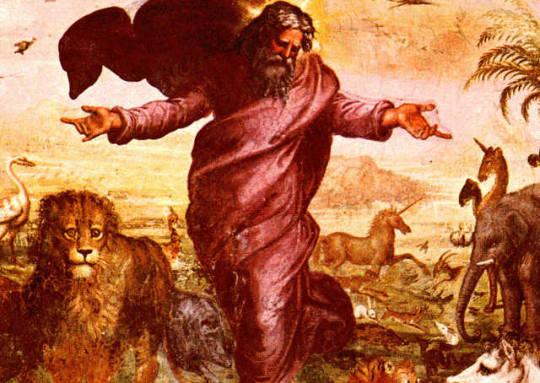
Book Of Genesis - From The Latin Vulgate - Chapter 15

INTRODUCTION.

The Hebrews now entitle all the Five Books of Moses, from the initial words, which originally were written like one continued word or verse; but the Sept. have preferred to give the titles the most memorable occurrences of each work. On this occasion, the Creation of all things out of nothing, strikes us with peculiar force. We find a refutation of all the heathenish mythology, and of the world’s eternity, which Aristotle endeavoured to establish. We behold the short reign of innocence, and the origin of sin and misery, the dispersion of nations, and the providence of God watching over his chosen people, till the death of Joseph, about the year 2369 (Usher) 2399 (Sal. and Tirin) B.C. 1631. We shall witness the same care in the other Books of Scripture, and adore his wisdom and goodness in preserving to himself faithful witnesses, and a true Holy Catholic Church, in all ages, even when the greatest corruption seemed to overspread the land. H.

—————————-

This Book is so called from its treating of the Generation, that is, of the Creation and the beginning of the world. The Hebrews call it Bereshith, from the word with which it begins. It contains not only the History of the Creation of the World, but also an account of its progress during the space of 2369 years, that is, until the death of Joseph.

The additional Notes in this Edition of the New Testament will be marked with the letter A. Such as are taken from various Interpreters and Commentators, will be marked as in the Old Testament. B. Bristow, C. Calmet, Ch. Challoner, D. Du Hamel, E. Estius, J. Jansenius, M. Menochius, Po. Polus, P. Pastorini, T. Tirinus, V. Bible de Vence, W. Worthington, Wi. Witham. — The names of other authors, who may be occasionally consulted, will be given at full length.

Verses are in English and Latin. HAYDOCK CATHOLIC BIBLE COMMENTARY

This Catholic commentary on the Old Testament, following the Douay-Rheims Bible text, was originally compiled by Catholic priest and biblical scholar Rev. George Leo Haydock (1774-1849). This transcription is based on Haydock’s notes as they appear in the 1859 edition of Haydock’s Catholic Family Bible and Commentary printed by Edward Dunigan and Brother, New York, New York.

TRANSCRIBER’S NOTES

Changes made to the original text for this transcription include the following:

Greek letters. The original text sometimes includes Greek expressions spelled out in Greek letters. In this transcription, those expressions have been transliterated from Greek letters to English letters, put in italics, and underlined. The following substitution scheme has been used: A for Alpha; B for Beta; G for Gamma; D for Delta; E for Epsilon; Z for Zeta; E for Eta; Th for Theta; I for Iota; K for Kappa; L for Lamda; M for Mu; N for Nu; X for Xi; O for Omicron; P for Pi; R for Rho; S for Sigma; T for Tau; U for Upsilon; Ph for Phi; Ch for Chi; Ps for Psi; O for Omega. For example, where the name, Jesus, is spelled out in the original text in Greek letters, Iota-eta-sigma-omicron-upsilon-sigma, it is transliterated in this transcription as, Iesous. Greek diacritical marks have not been represented in this transcription.

Footnotes. The original text indicates footnotes with special characters, including the astrisk (*) and printers’ marks, such as the dagger mark, the double dagger mark, the section mark, the parallels mark, and the paragraph mark. In this transcription all these special characters have been replaced by numbers in square brackets, such as [1], [2], [3], etc.

Accent marks. The original text contains some English letters represented with accent marks. In this transcription, those letters have been rendered in this transcription without their accent marks.

Other special characters.

Solid horizontal lines of various lengths that appear in the original text have been represented as a series of consecutive hyphens of approximately the same length, such as .

Ligatures, single characters containing two letters united, in the original text in some Latin expressions have been represented in this transcription as separate letters. The ligature formed by uniting A and E is represented as Ae, that of a and e as ae, that of O and E as Oe, and that of o and e as oe.

Monetary sums in the original text represented with a preceding British pound sterling symbol (a stylized L, transected by a short horizontal line) are represented in this transcription with a following pound symbol, l.

The half symbol (½) and three-quarters symbol (¾) in the original text have been represented in this transcription with their decimal equivalent, (.5) and (.75) respectively.

Unreadable text. Places where the transcriber’s copy of the original text is unreadable have been indicated in this transcription by an empty set of square brackets, [].

Chapter 15

God promiseth seed to Abram. His faith, sacrifice and vision.

[1] Now when these things were done, the word of the Lord came to Abram by a vision, saying: Fear not, Abram, I am thy protector, and thy reward exceeding great. His itaque transactis, factus est sermo Domini ad Abram per visionem dicens : Noli timere, Abram : ego protector tuus sum, et merces tua magna nimis.

[2] And Abram said: Lord God, what wilt thou give me? I shall go without children: and the son of the steward of my house is this Damascus Eliezer. Dixitque Abram : Domine Deus, quid dabis mihi? ego vadam absque liberis, et filius procuratoris domus meae iste Damascus Eliezer.

[3] And Abram added: But to me thou hast not given seed: and lo my servant, born in my house, shall be my heir. Addiditque Abram : Mihi autem non dedisti semen, et ecce vernaculus meus, haeres meus erit.

[4] And immediately the word of the Lord came to him, saying: He shall not be thy heir: but he that shall come out of thy bowels, him shalt thou have for thy heir. Statimque sermo Domini factus est ad eum, dicens : Non erit hic haeres tuus, sed qui egredietur de utero tuo, ipsum habebis haeredem.

[5] And he brought him forth abroad, and said to him: Look up to heaven and number the stars, if thou canst. And he said to him: So shall thy seed be. Eduxitque eum foras, et ait illi : Suscipe caelum, et numera stellas, si potes. Et dixit ei : Sic erit semen tuum.

[6] Abram believed God, and it was reputed to him unto justice. Credidit Abram Deo, et reputatum est illi ad justitiam.

[7] And he said to him: I am the Lord who brought thee out from Ur of the Chaldees, to give thee this land, and that thou mightest possess it. Dixitque ad eum : Ego Dominus qui eduxi te de Ur Chaldaeorum ut darem tibi terram istam, et possideres eam.

[8] But he said: Lord God, whereby may I know that I shall possess it? At ille ait : Domine Deus, unde scire possum quod possessurus sim eam?

[9] And the Lord answered, and said: Take me a cow of three years old, and a she goat of three years, and a ram of three years, a turtle also, and a pigeon. Et respondens Dominus : Sume, inquit, mihi vaccam trienem, et capram trimam, et arietem annorum trium, turturem quoque et columbam.

[10] And he took all these, and divided them in the midst, and laid the two pieces of each one against the other; but the birds he divided not. Qui tollens universa haec, divisit ea per medium, et utrasque partes contra se altrinsecus posuit; aves autem non divisit.

[11] And the fowls came down upon the carcasses, and Abram drove them away. Descenderuntque volucres super cadavera, et abigebat eas Abram.

[12] And when the sun was setting, a deep sleep fell upon Abram, and a great and darksome horror seized upon him. Cumque sol occumberet, sopor irruit super Abram, et horror magnus et tenebrosus invasit eum.

[13] And it was said unto him: Know thou beforehand that thy seed shall be a stranger in a land not their own, and they shall bring them under bondage, and afflict them four hundred years. Dictumque est ad eum : Scito praenoscens quod peregrinum futurum sit semen tuum in terra non sua, et subjicient eos servituti, et affligent quadringentis annis.

[14] But I will judge the nation which they shall serve, and after this they shall come out with great substance. Verumtamen gentem, cui servituri sunt, ego judicabo : et post haec egredientur cum magna substantia.

[15] And thou shalt go to thy fathers in peace, and be buried in a good old age. Tu autem ibis ad patres tuos in pace, sepultus in senectute bona.

[16] But in the fourth generation they shall return hither: for as yet the iniquities of the Amorrhites are not at the full until this present time. Generatione autem quarta revertentur huc : necdum enim completae sunt iniquitates Amorrhaeorum usque ad praesens tempus.

[17] And when the sun was set, there arose a dark mist, and there appeared a smoking furnace and a lamp of fire passing between those divisions. Cum ergo occubuisset sol, facta est caligo tenebrosa, et apparuit clibanus fumans, et lampas ignis transiens inter divisiones illas.

[18] That day God made a covenant with Abram, saying: To thy seed will I give this land, from the river of Egypt even to the great river Euphrates. In illo die pepigit Dominus foedus cum Abram, dicens : Semini tuo dabo terram hanc a fluvio Aegypti usque ad fluvium magnum Euphraten,

[19] The Cineans and Cenezites, the Cedmonites, Cinaeos, et Cenezaeos, Cedmonaeos,

[20] And the Hethites, and the Pherezites, the Raphaim also, et Hethaeos, et Pherezaeos, Raphaim quoque,

[21] And the Amorrhites, and the Chanaanites, and the Gergesites, and the Jebusites. et Amorrhaeos, et Chananaeos, et Gergesaeos, et Jebusaeos.

Commentary:

Ver. 1. Fear not. He might naturally be under some apprehensions, lest the four kings should attempt to be revenged upon him. --- Reward, since thou hast so generously despised earthly riches. H. --- Abram was not asleep, but saw a vision of exterior objects. v. 5.

Ver. 2. I shall go. To what purpose should I heap up riches, since I have no son to inherit them? Abram knew that God had promised him a numerous posterity; but he was not apprized how this was to be verified, and whether he was to adopt some other for his son and heir. Therefore, he asks modestly, how he out to understand the promise. --- And the son, &c. Heb. is differently rendered, "and the steward of my house, this Eliezer of Damascus." We know not whether Eliezer or Damascus be the proper name. The Sept. have "the son of Mesech, my handmaid, this Eliezer of Damascus." Most people suppose, that Damascus was the son of Eliezer, the steward. The sentence is left unfinished, and must be supplied from the following verse, shall be my heir. The son of the steward, filius procurationis, may mean the steward himself, as the son of perdition denotes the person lost. C.

Ver. 6. Reputed by God, who cannot judge wrong; so that Abram increased in justice by this act of faith, believing that his wife, now advanced in years, would have a child; from whom others should spring, more numerous than the stars of heaven. H. --- This faith was accompanied and followed by many other acts of virtue. S. Jam. ii. 22. W.

Ver. 8. Whereby, &c. Thus the blessed Virgin asked, how shall this be done? Lu. i. 34. without the smallest degree of unbelief. Abram wished to know, by what signs he should be declared the lawful owner of the land. H.

Ver. 9. Three years, when these animals have obtained a perfect age.

Ver. 12. A deep sleep, or ecstasy, like that of Adam. G. ii. 21, wherein God revealed to him the oppression of his posterity in Egypt, which filled him with such horror (M.) as we experience when something frightful comes upon us suddenly in the dark. This darkness represents the dismal situation of Joseph, confined in a dungeon; and of the Hebrews condemned to hard labour, in making bricks, and obliged to hide their male children, for fear of their being discovered, and slain. Before these unhappy days commenced, the posterity of Abram were exposed to great oppression among the Chanaanites, nor could they in any sense be said to possess the land of promise, for above 400 years after this prophetic sleep. H.

Ver. 13. Strangers, and under bondage, &c. This prediction may be dated from the persecution of Isaac by Ismael, A. 2112, till the Jews left Egypt, 2513. In Exodus xii. and S. Paul, 430 years are mentioned; but they probably began when Abram went first into Egypt, 2084. Nicholas Abram and Tournemine say, the Hebrews remained in Egypt full 430 years. from the captivity of Joseph; and reject the addition of the Sept. which adds, "they and their fathers dwelt in Egypt, and in Chanaan." On these points, we may expect to find chronologists at variance.

Ver. 14. Judge and punish the Egyptians, overwhelming them in the Red sea, &c. H.

Ver. 16. Fourth, &c. after the 400 years are finished; during which period of time, God was pleased to bear with those wicked nations; whose iniquity chiefly consisted in idolatry, oppression of the poor and strangers, forbidden marriages of kindred, and abominable lusts. Levit. xviii. Deut. vi. and xii. M.

Ver. 17. A lamp, or symbol of the Divinity, passing, as Abram also did, between the divided beasts, to ratify the covenant. See Jer. xxxiv. 18.

Ver. 18. Of Egypt, a branch of the Nile, not far from Pelusium. This was to be the southern limit, and the Euphrates the northern; the two other boundaries are given, Num. xxxiv. --- Perhaps Solomon's empire extended so far. At least, the Jews would have enjoyed these territories, if they had been faithful. M.

Ver. 19. Cineans, in Arabia, of which nation was Jethro. They were permitted to dwell in the tribe of Juda, and served the Hebrews. --- Cenezites, who probably inhabited the mountains of Juda. --- Cedmonites, or eastern people, as their name shews. Cadmus was of this nation, of the race of the Heveans, dwelling in the environs of mount Hermon, whence his wife was called Hermione. He was, perhaps, one of those who fled at the approach of Josue; and was said to have sowed dragons' teeth, to people his city of Thebes in Beotia, from an allusion to the name of the Hevites, which signifies serpents. C. --- The eleven nations here mentioned were not all subdued; on account of the sins of the Hebrews. M.

[testblogplzignore]

I used that necessary boundary condition

http://jwilson.coe.uga.edu/EMT668/EMAT6680.2003.Su/Daly/write_ups/WR_12/Asmt_12.htm

The assumptions for this are spicy and quite amusing so if I can get it to work I can show direct numbers/functions. Legit making me laugh thinking about it and what you’d physically have to do. If it doesn’t work I’ll tell you in this post

\( f(x) = H(x) \)

where

\( H(x) = 0\) when \( x=h=0\) and \(  H(x) = T_1 \) when \( 0<x<h \)

\( w(x,t) = f(x)-\Big[ \frac{T_2 - T_1}{h} x + T_1 \Big] \)

\( w(x,t) = H(x)-\Big[ \frac{T_2 - T_1}{h} x + T_1 \Big] \)

\( w(0,t) = w(h,t) = 0 \) indeed (how did I not notice this egregious mistake)

\( w(x,0) = H(x) -  \Big[ \frac{T_2 - T_1}{h} x + T_1 \Big] \)

\( w(x,0) = H(x) +  \frac{T_1 - T_2}{h} x - T_1 \)

\( c_n = \frac{2}{h} \int_{0}^{h}  w(x,0)  sin \big( \frac{n \pi x}{h} \big)dx \)

\( c_n = \frac{2}{h} \int_{0}^{h}  \Big[   H(x) +  \frac{T_1 - T_2}{h} x - T_1 \Big] sin \big( \frac{n \pi x}{h} \big)dx \)

\( c_n = \frac{2}{h}\Big[ \int_{0}^{h}   H(x) sin \big( \frac{n \pi x}{h} \big) dx  +   \frac{T_1 - T_2}{h} \int_{0}^{h} x sin \big( \frac{n \pi x}{h} \big)dx - T_1 \int_{0}^{h} sin \big( \frac{n \pi x}{h} \big)    dx \Big] \)

first integral

\( \int_{0}^{h}   H(x) sin \big( \frac{n \pi x}{h} \big) dx = 0 \) by space

Just goes to show brute forcing is legit retarded. I missed it in my notes so I got punished. Also we have

\( \frac{\partial}{\partial t} w(x,t) = \beta \frac{\partial^2}{\partial x^2} w(x,t) \) which is true because it’s not dependent on time and its spatial derivative the spatial Heaviside derivative is zero after the first. We have this because \( u(x) \) has no time dependence so left side is zero and it’s a straight line in one spatial dimension so double derivative is zero

\( T(x,t) = u(x) + w(x,t) \)

I see now why they characterize it with a function dependent on x only as the no function with dependence on t has the first derivative equal to zero which we require for this method. They could explain that or maybe they did and didn’t write it down for people who terribly take notes. Anyhoo

second integral

\( \frac{T_1 - T_2}{h} \int_{0}^{h} x sin \big( \frac{n \pi x}{h} \big)dx =   \frac{T_1 - T_2}{h} \Big[ \frac{h^2}{(n \pi )^2} \big[ sin \big( \frac{n \pi x}{h} \big)- \frac{n \pi x}{h} cos \big( \frac{n \pi x}{h}   \big)\big] \Big]_{0}^{h} \)

Gonna show full steps in case this one works (it should by the extra condition I saw but I’ve done this integration before and it didn’t work out, can try small angle to see if it does and also can put faith in the Fourier decomposition and taking a specific n doesn’t necessarily have to cancel off in that term)

Notice at \( sin \big( \frac{n \pi x}{h} \big) \Big|_0^h \) you get \( sin \big( \frac{n \pi h}{h} \big)  - sin \big( n \pi 0 \big) \) and since we’re summing over n that first term always goes to zero hence

\( sin \big( \frac{n \pi x}{h} \big) \Big|_0^h =0 \)

\( \Big[  \frac{n \pi x}{h} cos \big( \frac{n \pi x}{h}  \big) \Big]_0^h =  - \frac{n \pi h}{h} cos \big( \frac{n \pi h}{h} \big) -  - \frac{n \pi 0}{h} cos \big( \frac{n \pi 0}{h} \big)  \)

As you can see the right term goes to zero (I believe at this point being this in detail is retarded) and the left term is proportionate to \( cos ( n \pi ) \) which again is being summed over so it’s always equal to \( 1 \)

\( \Big[  \frac{n \pi x}{h} cos \big( \frac{n \pi x}{h} \big) \Big]_0^h =    - n \pi   \)

third integral

  \( - T_1 \int_{0}^{h} sin \big( \frac{n \pi x}{h} \big)   dx = 0 \) by space

so final form looks like

\( c_n = \frac{2}{h}\Big[ \int_{0}^{h}   H(x) sin \big( \frac{n \pi x}{h} \big) dx  +   \frac{T_1 - T_2}{h} \int_{0}^{h} x sin \big( \frac{n \pi x}{h} \big)dx - T_1 \int_{0}^{h} sin \big( \frac{n \pi x}{h} \big)   dx \Big]  \)

\( c_n = \frac{2}{h} \frac{T_1 - T_2}{h} \frac{h^2}{(n \pi )^2}(- n \pi  ) \)

\( c_n = \frac{2}{h} \frac{T_2 - T_1}{h} \frac{h^2}{(n \pi )^2}( n \pi  ) \)

\( c_n = \frac{2(T_2 - T_1)}{n \pi} \)

\( w(x,t) = \sum_{n=1}^{\infty} c_n sin \big( \frac{n \pi x}{h} \big) e^{-\beta \Big( \frac{n \pi}{h} \Big)^2 t} \)

\( w(x,t) = \sum_{n=1}^{\infty} \frac{2(T_2 - T_1)}{n \pi} sin \big( \frac{n \pi x}{h} \big) e^{-\beta \Big( \frac{n \pi}{h} \Big)^2 t} \)

\( w(x,t) = \frac{2(T_2 - T_1)}{\pi} \sum_{n=1}^{\infty} \frac{1}{n} sin \big( \frac{n \pi x}{h} \big) e^{-\beta \Big( \frac{n \pi}{h} \Big)^2 t} \)

\( T(x,t) = \frac{2(T_2 - T_1)}{\pi} \sum_{n=1}^{\infty} \frac{1}{n} sin \big( \frac{n \pi x}{h} \big) e^{-\beta \Big( \frac{n \pi}{h} \Big)^2 t} + \frac{T_2 - T_1}{h} x + T_1 \)

\( T(0,t) = \frac{2(T_2 - T_1)}{\pi} \sum_{n=1}^{\infty} \frac{1}{n} sin \big( \frac{n \pi 0}{h} \big) e^{-\beta \Big( \frac{n \pi}{h} \Big)^2 t} + \frac{T_2 - T_1}{h} 0+ T_1 \)

\( T(0,t) = T_1 \)

\( T(h,t) = \frac{2(T_2 - T_1)}{\pi} \sum_{n=1}^{\infty} \frac{1}{n} sin \big( \frac{n \pi h}{h} \big) e^{-\beta \Big( \frac{n \pi}{h} \Big)^2 t} + \frac{T_2 - T_1}{h} h+ T_1 \)

\( T(h,t) =T_2 \)

\( T(x,0) = \frac{2(T_2 - T_1)}{\pi} \sum_{n=1}^{\infty} \frac{1}{n} sin \big( \frac{n \pi x}{h} \big) e^{-\beta \Big( \frac{n \pi}{h} \Big)^2 0} + \frac{T_2 - T_1}{h} x + T_1 \)

\( T(x,0) = \frac{2(T_2 - T_1)}{\pi} \sum_{n=1}^{\infty} \frac{1}{n} sin \big( \frac{n \pi x}{h} \big) + \frac{T_2 - T_1}{h} x + T_1 \)

Let’s check \( n=1 \)

\( T(x,0) \Big|_{n=1} = \frac{2(T_2 - T_1)}{\pi} \sum_{n=1}^{1} \frac{1}{n} sin \big( \frac{n \pi x}{h} \big) + \frac{T_2 - T_1}{h} x + T_1 \)

\( T(x,0) \Big|_{n=1} = \frac{2(T_2 - T_1)}{\pi} \frac{1}{1} sin \big( \frac{1 \pi x}{h} \big) + \frac{T_2 - T_1}{h} x + T_1 \)

\( T(x,0) \Big|_{n=1} = \frac{2(T_2 - T_1)}{\pi}  sin \big( \frac{ \pi x}{h} \big) + \frac{T_2 - T_1}{h} x + T_1 \)

small angle approximation says

\( sin(\theta ) \approx \theta\) so

\( T(x,0) \Big|_{n=1} \approx \frac{2(T_2 - T_1)}{\pi} \frac{ \pi x}{h} + \frac{T_2 - T_1}{h} x + T_1  \)

\( T(x,0) \Big|_{n=1} \approx \frac{  2(T_2 - T_1) }{h}x + \frac{T_2 - T_1}{h} x + T_1 \) 

well shit

\( T(x,0) \Big|_{n=1} \approx   3\frac{T_2 - T_1}{h} x + T_1 \)

Let’s invoke some physicality or bullshit, \( f(x) \) says the temperature of our coffee is exactly \( T_1 \) everywhere in the cup except the endpoints being exactly \( 0 \). Physically we take this to mean that \( T_1 = T_2 \) at exactly \( T(x,0) \) so (again I completely missed it

\( T(x,0) \Big|_{n=1} \approx T_1 \) which is our initial condition

fuck that feels good

so

\( T(x,t) = \frac{2(T_2 - T_1)}{\pi} \sum_{n=1}^{\infty} \frac{1}{n} sin \big( \frac{n \pi x}{h} \big) e^{-\beta \Big( \frac{n \pi}{h} \Big)^2 t} + \frac{T_2 - T_1}{h} x + T_1 \)

Technically if you were to graph this it would be flat for a millisecond then one fixed endpoint (in our case at \(h\)) you’d see an instantaneous drop on one side to \( T_2 \) and then the heat traveling through it from the cold side to the warm side like the opposite of this graph (going into more detail in my actual post and not shitty latex posts

The way this would be achieved is physically impossible but let’s see your coffee cup

started at 4:27 am took way too long for such a simple pde but damn does the latex take work

8:36 am turns out every single time I typed \( T(x,t) \) it was missing a negative sign in the exponential. Fixing for this post and probably the other one where I make the actual post

9:40 am

fug maple says it’s wrong

shouldn’t have tried to bullshit the obvious contradiction

9:58 am I see it’s because I did the Fourier decomposition of only the steady state solution without a term to offset that. XD

I’m at a point where I’m starting to see it as too complex for an analytical solution

10:13 considering dropping the physicality just so i can do it

It’s the mother fucking Fourier decomposition that fucks this. Perhaps I do actually need to do separation of variables but again I need homogeneous boundary conditions in at least one dimension

12:39 pm

aight might as well tell you. Sadge about thinking I solved it. Anyway it required the ice cube to melt literally instantly and required constant ice pouring at the top of the coffee to consistently keep it this temperature. Now that I think about it an insulated coffee makes more sense with an impulse for the ice. I thought it was amusing thinking of somebody constantly putting in ice to keep the temperature constant. Probably only me who finds it that amusing. Likewise it required the bottom of the coffee to be constantly heated to a certain temperature. The other assumptions are on the original post. I suppose I should do something with my time

12:27 am 21/08/04

Did I fuck up my step function. It was supposed to have \( H(0)=T_1 \) instead of \( 0 \)

The fixes the integral and you have an offset term. Let me try putting it into maple

12:29 am

No because the integral still goes to zero for that step function. I wonder if it makes a difference for insulated endpoints. I don’t see why it would and it would probably still fail

12:46 am

It occurs to me that I messed up my step function and am writing it down on paper now

1:24 am

This is actually the solution I just messed up my \( H(x) \) which is actually just a step function instead of the Heaviside function. I had multiple warnings too at both the bullshit step and the initial checking that \( w(0,t) = w(h,t)=0 \)

12:00 pm 21/08/04

Is very close to if not the right answer. Maple doesn’t like the step function so it bugs out. I did multiple integrals and one of them is right

[mathematicianadda]

A circle is divided into $5$ parts as shown in the diagram and parts are colored either red or green. Find which area is bigger. https://ift.tt/2PeDy6n

In the given diagram, there are $5$ points $A, B, C, D$ and $E$ on the circumference of the circle such that $\angle ABC = \angle BCD = \angle CDE = 45^{\circ}$ and $O$ is the center of the circle.

Sectors made by $AB$ and $DE$, and area of the circle between $BC$ and $CD$ are highlighted in green. Area of the circle between $AB$ and $BC$, and between $CD$ and $DE$ are highlighted in red.

Which area is bigger, the area highlighted in red or the area highlighted in green?

This was sent to me by someone. While I solved the problem (given below), the sender said that the source solution arrived at the conclusion that points $A$, $O$ and $E$ are collinear and $OC \perp AE$, so $\displaystyle \angle OCB = \angle OCD = \frac{45^{\circ}}{2}=22.5^{\circ}$. While I agree with points being collinear and $OC \perp AE$ but that cannot obviously be the reason for the angles being equal. In fact the solution does not depend on them being equal as we can see. I am seeking help in establishing $\angle OCB = \angle OCD$ if that is indeed true, which I cannot see how one can conclude based on what is given.

My solution: Say, $\angle OCB = \theta$. Then, $\angle ACB = \angle OCD = (45^{\circ}-\theta)$ and $\angle DCE = \theta$.

Segment $AB= \displaystyle r^2 \left[\frac{\pi}{4}-\theta-\sin(45^{\circ}-\theta)\cos(45^{\circ}-\theta)\right]$ Segment $DE= \displaystyle r^2 \left[\theta-\sin \theta \cos \theta\right]$

$\triangle OBC = r^2 \sin \theta \cos \theta$ $\triangle ODC = r^2 \sin(45^{\circ}-\theta)\cos(45^{\circ}-\theta)$

Section $BOD = \dfrac{\pi}{4} r^2$

Adding all of the above, total area in green $= \dfrac{\pi}{2} r^2$. So the red area has to be the same too.

In addition to my question on $OC$ being bisector of $\angle BCD$, let me also know if any of you have a simpler solution.

from Hot Weekly Questions - Mathematics Stack Exchange Math Lover from Blogger https://ift.tt/3fjqLu1

[fxcfdlabo]

トレンドを見極める方法の一つとして、オシレーターでギャンファンを利用してみよう！AXIORYで、Autochartistを利用しよう！！

株式投資や、為替取引をするとき、価格の強気下落中の下降トレンドへの投資は、かなり人気のある長期戦略です。なぜなら、安売りバーゲンセールだからです。日本円を売って米ドルを買うという通貨ペア 「USD / JPY」や、もしくは、長期の強気トレンドにある他の通貨ペアに注目し、下落してジャンプするのを待ちます。通貨ペアが低いときに買い、上昇トレンドが続き、利益確定を待ちます。 しかし、「安く買って高く売ればいい」と口で言うのは簡単ですが、安値で通貨を買って、逆に損失が膨らんだというトレーダーが多いのも現状です。 少しの価格下落が、ストップロス(ロスカット, 損切り)に達するまでどんどん強くなり、ストップロスされ、市場から強制退場させられます。 そして、思ったようにうまくいかない事象は、何でも間違ってしまうという「マーフィーの法則」が発動し、ストップロス(ロスカット, 損切り)された後、上昇し始め、損してしまうトレーダーもたくさんいます。 我々投資家に必要なのは、我々がいつ、通貨を買うという「エントリー」をして、強制ロスカットされることなく強気のトレンドに乗ることができるように、どのくらいの強い相場なのかを把握することです。 このブログの管理人がトレンドを見極めるのに効果的だと思う戦術の1つは、「ギャンファン」と「オシレーター」を組み合わせることです。 これにより、下落相場で通貨を購入する適切なタイミングを、より高い精度で予測できます。

全てのギャンファンには、オシレーターが必要だ

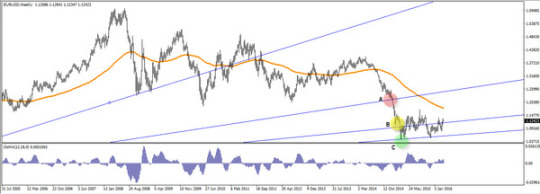
ギャンファンの仕組みは非常に簡単です。 下の図のように、トレンド全体のトレンドラインサポートとしてメインギャンラインを引き伸ばし、「ギャンファン」という概念を使用すると、上下の代替トレンドラインが得られます。 しかし、「ギャンファン」という概念を利用するときの一番の難しいことは、どの代替トレンドラインが実際に保持され、トレンドを継続できるかを判断することです。 「ギャンファン」を利用すると、今までよりもトレンドを見極めやすくなります。 それにもかかわらず、ギャンファンをオシレーターと組み合わせると、ギャンファンは、はるかに正確になります。 ギャンファンと同時に、使用できるオシレーターは、MACD、ストキャスティックオシレーター、移動平均オシレーターなどです。 以下の図を見ると、ギャンファンがトレンドの転換である可能性と思われる3つのポイント「A、B、C」を暗示していることがわかります。 A地点とB地点では、トレンドが上昇すると思われても下降してしまう「だまし」ですが、Cはトレンド転換点です。 C地点でのみ、オシレーターが負から正に移動し、運動量の変化を示唆し、これが真の支持線であることを示します。

「だまし」を避ける3つのコツとは?

ギャンファンを利用するとき、他のテクニカル分析と同様に、「落とし穴」や「だまし」を見分けるために、最善の注意を払わなければなりません。 最も一般的な「だまし」を回避するためのいくつかのトリックを以下に示します。

ギャンファンのチェック

はじめに確認しなければならないことは、主要トレンドラインの上に「ギャンファン」のメインラインを描いたことです。 トレンドの転換点から、以下の図のようにギャンラインを描く必要があります。これは、以下の図に示すように、上昇トレンドか下降トレンドかを認識するための主な「トレンドライン」を目視して理解するのに役立ちます。

スキャルビングや、数分程度の短期トレードで「ギャンファン」を利用しない

「ギャンファン」を1時間以下の短い間隔で測定することは可能ですが、これらの短期間では、オシレーターの効果ははるかに低くなります。 また、オシレーターと併用することによってギャンファンの精度が向上するので、オシレーターがない短期間では、ギャンファンの精度が大幅に低下します。この場合は、「ギャンファン」は利用せずに、異なるストラテジーとテクニカル分析を使用しましょう。

通貨ペアに注意

オシレーターと親和性のある「ギャンファン」を使って分析する最大のリスクの1つは、トレンドが強気から弱気に変わった場合、ギャンの支持線や抵抗線を突破して価格が動いてしまうことです。 トレンドの変化を見極めることができない場合や、ペアが2〜3回、「ギャンファン」の支持線や抵抗線を上回らなかった場合には、警告サインが表示されます。 これは、ペアの抵抗が大きいことを示しています。 トレンドがまだ強気もしくは弱気であることを少なくとも二重にチェックした方がリスク回避につながります。トレンドの認識に対して確実な確信が持てない場合は、取引を一時期休止して、様子を見ることも必要です。

「ギャンファン」とは?

ギャンファンとは、株式取引やFX取引をするための取引市場の価格が、本質的に幾何学的かつ周期的であるという考えに基づいたテクニカル分析の一つです。 ギャンファンは、「ギャンアングル」と呼ばれる一連の線で構成されます。 これらの角度は、潜在的な支持線と抵抗線を示すために価格チャートに重ねられます。 以下の画像は、トレンドの変換点での、数分という短期間ではない近未来の価格の変化を予測するのに、「ギャンファン」が役立ちます。

ギャンファンの主なポイント

・ギャンファンは、W.D. Gannによって開発されました。 ・ギャンファンはトレンド転換点を原点とする「直線」です。 ユーザーが開始点を選択すると、線が未来に延長されます。 ・ギャンファンは、45°の角度を中心にして、度数法で表されたおおよその角度「82.5°、75°、71.25°、63.75°、26.25°、18.75°、15°、7.5°」を描写。 ・ギャンファンは、低または高ポイントで開始されます。 結果の行は、将来の潜在的なサポートと抵抗の領域を示しています。

ギャンファンがトレーダーに伝える内容とは?

トレンドの方向と強さを判断するために、中央の45度の線の上下に斜めの線が引かれています。 ギャンファンは。「W. D. Gann」によって開発されました。時間と価格のバランスに関する理論に基づいて、トレンドの転換点を原点として、そこから引いた直線から45度の角度がチャート作成に理想的な角度であるとW. D. Gannは、主張しています。 ギャンファンは、指定されたトレンド反転レベルから伸びる中央の45度の角度線から描画されます。トレーダーは反転点でギャンファンを引き寄せ、支持線と抵抗線の位置が、将来に拡大することを確認します。 ギャンファンの45度の角度線は、チャート上の45度の角度に揃える必要があります。 45度の角度を見つけるには、グラフ作成プラットフォームで角度ツールを使用します。

45度の線は1：1の線として知られています。これは、価格が単位時間ごとに1単位上下するときに価格が45度の角度で上下するためです。 ギャンファンファンの他のすべての線は、1：1の線の上下に描かれます。トレーダーは、ギャンファンチャートの1：1の線の上下にさまざまな数の線を使用できます。その他の角度は、2：1、3：1、4：1、8：1と、1：1の線の境にして、1：8、1：4、1：3、1：2の価格設定時間の動きに関連付けられています。 1：1行が主要な指標です。ただし、チャーティストは、独自の裁量で行を追加する選択肢があります。上昇トレンドと下降トレンドの両方で、1：1線は反転を検出するのに役立ちます。下降トレンドでは、1：1線を下回る価格は弱気とみなされます。上昇トレンドでは、1：1ラインを上回ったままの価格は強気と見なされます。したがって、1：1ラインは抵抗線およびサポート線として機能します。

ギャンファンが描かれた追加の線は、抵抗線およびサポート線としても使用されます。ギャンは、価格が1つの角度を移動した場合、次の角度に向かう可能性が高いと考えていました。たとえば、価格が45度の角度（1：1）を下回ると、26.25度の角度（2：1）に下がります。価格が1：1を下回っても、必ずしも全体的な上昇トレンドが終わったわけではありません。価格は2：1でサポートされ、その後上昇し続ける可能性があります。そうは言っても、価格が2：1の線に下がった場合、1：1未満の下落は少なくとも短期的な弱さを示す可能性があります。

ギャンファン利用時の「ギャンアングル」の計算方法

ギャンファンを利用するとき、傾斜角度である「ギャンアングル」\( \theta \)を理解しなければなりません。 \( xy \)平面に置ける格子点に置いて、 正方形の一片を単位時間とすると、その単位時間内に価格が正方形の高さまで上昇する場合、正方形の左下から右上に線を引くことができます。 その線の傾斜度は45°になります。 1つのボックスの高さを上げるのに2つの正方形が必要な場合は、2：1であり、上昇角度は45度よりも平坦になります。 1つのボックスの時間枠が1：2の間で価格が2つのボックスの高さまで上昇する場合は、その角度は45度よりも急な傾きになります。 ギャンファンには、価格と時間の比率の動きに基づく角度が次の比率で組み込まれています。 ・1：8の場合は「82.5°」 ・1：4の場合は「75°」 ・1：3の場合は「71.25°」 ・1：2の場合は「63.75°」 ・1：1の場合は「45°」 ・2：1の場合は「26.25°」 ・3：1の場合は「18.75°」 ・4：1の場合は「15°」 ・8：1の場合は「7.5°」 となります。この角度はテクニカル分析を利用している投資家にはよく知られている角度ですが、この角度は、厳密には違います。つまり、上記の角度は、数学的には、不正確なのです。 トレンド転換点からの単位時間を\( x\)とし、トレンド転換点からの価格を\(y \)とし、ギャンアングルを\( \theta \)とすると、以下の式が成り立ちます。 \[ \tan \theta=\frac{y}{x} \] この\( \theta\)を正確に求める必要があります。正確さこそが、トレンドを正確に測るのに必要だからです。 任意の実数\(x \)に対して、\(\tan x \)は、周期\( \pi \)を持ち、任意の整数\( n\)に対して、\(x= \frac{\pi}{2}+n\pi \)では定義することはできません。そこで、\(-\frac{\pi}{2} \[ \frac{d}{dx}(\tan x)=\frac{1}{\cos^{2}x} > 0 \] が成り立つので、狭義単調増加します。したがって、関数\( f(x)=\tan x \)を表す写像 \[ f: ( -\pi /2, \pi /2 ) \rightarrow ( -\infty, \infty ) \] は、全単射となるので、任意の実数\( y\)に対して、\( y=\tan x \)となる\( x\in ( -\pi /2, \pi /2 ) \)がただ一つ存在します。したがって、\( \tan x \)は、\(-\frac{\pi}{2} すると、トレンド転換点からの単位時間\( x\)と、トレンド転換点からの価格\(y \)に対して、求めるギャンアングル\( \theta \)は、 \[ \theta =\arctan \frac{y}{x} \] となります。よく知られている値は、 \[ \begin{eqnarray} &\arctan 1=\frac{\pi}{4},\ \arctan \frac{1}{\sqrt{3}}=\frac{\pi}{6},\ \arctan \sqrt{3}=\frac{\pi}{3},\ \arctan 0=0&\\ &\arctan (-1)=-\frac{\pi}{4},\ \arctan \left(-\frac{1}{\sqrt{3}} \right)=-\frac{\pi}{6},\ \arctan (-\sqrt{3})=-\frac{\pi}{3}&\\ \end{eqnarray} \] ぐらいです。つまり、任意の実数\( x\)に対して、\( \arctan x \)を具体的に求めるのは、難しいと思われます。そこで、以下の冪級数を利用します。 \[ \arctan x=\int_{0}^{x}\frac{dt}{1+t^{2}}=\sum_{n=0}^{\infty}\frac{(-1)^{n}}{2n+1}x^{2n+1}, \quad (-1\leq x \leq 1) \] しかし、上記の冪級数は、\(-1\leq x \leq 1 \)でしか定義されていないので、\(x \[ \arctan x+\arctan \frac{1}{x}=\frac{\pi}{2} \] が成り立つことを利用すれば、\(x すると、以下のように、比較的に精度の高いギャンアングルが得られます。 \[ \begin{eqnarray} &\arctan \frac{1}{8}=\sum_{n=0}^{\infty}\frac{(-1)^{n}}{2n+1} \left(\frac{1}{8} \right)^{2n+1}=0.1243549945\cdots &\\ &\arctan \frac{1}{4}=\sum_{n=0}^{\infty}\frac{(-1)^{n}}{2n+1} \left(\frac{1}{4} \right)^{2n+1}=0.2449786631\cdots &\\ &\arctan \frac{1}{3}=\sum_{n=0}^{\infty}\frac{(-1)^{n}}{2n+1} \left(\frac{1}{3} \right)^{2n+1}=0.3217505544\cdots &\\ &\arctan \frac{1}{2}=\sum_{n=0}^{\infty}\frac{(-1)^{n}}{2n+1} \left(\frac{1}{2} \right)^{2n+1}=0.463647609\cdots &\\ &\arctan 2=\frac{\pi}{2}-\arctan \frac{1}{2}=1.107148718\cdots &\\ &\arctan 3=\frac{\pi}{2}-\arctan \frac{1}{3}=1.249045772\cdots &\\ &\arctan 4=\frac{\pi}{2}-\arctan \frac{1}{4}=1.325817664\cdots &\\ &\arctan 8=\frac{\pi}{2}-\arctan \frac{1}{8}=1.446441332\cdots &\\ \end{eqnarray} \] となります。ここで注意すべきことは、上記で計算した\( \arctan\)の値が、実数値(弧度法)であり、度数法ではないということです。従って、上記の値に\( 180/\pi\)をかける必要があります。すると、 \[ \begin{eqnarray} &\arctan \frac{1}{8}=0.1243549945\cdots \times \frac{180}{\pi}=7.125016349\cdots ^{ \circ } &\\ &\arctan \frac{1}{4}=0.2449786631\cdots \times \frac{180}{\pi}=14.03624347\cdots ^{ \circ }&\\ &\arctan \frac{1}{3}=0.3217505544\cdots \times \frac{180}{\pi}=18.43494882\cdots ^{ \circ }&\\ &\arctan \frac{1}{2}=0.463647609\cdots \times \frac{180}{\pi}=26.56505118\cdots ^{ \circ }&\\ &\arctan 2=1.107148718\cdots \times \frac{180}{\pi}=63.43494882\cdots ^{ \circ }&\\ &\arctan 3=1.249045772\cdots \times \frac{180}{\pi}=71.56505118\cdots ^{ \circ }&\\ &\arctan 4=1.325817664\cdots \times \frac{180}{\pi}=75.96375653\cdots ^{ \circ }&\\ &\arctan 8=1.446441332\cdots \times \frac{180}{\pi}=82.87498365\cdots ^{ \circ }&\\ \end{eqnarray} \] となります。ギャンアングルの精度がかなり上がりましたが、小数点がずっと続いています。一体、上記の数がどのような数なのかをこの記事ではしっかりと調べていきます。 今、\( s > 0 \), \( t \geq 0 \)を整数として、0以上の整数\( n \)に対して、以下の漸化式を満たす数列\( \{a_{n} \}_{n=0}^{\infty} \)を以下のようにとります。 \[ \begin{eqnarray} &a_{0}=1,\ a_{1}=s&\\ &a_{n+2}-2sa_{n+1}+(s^{2}+t^{2})a_{n}=0& \end{eqnarray} \] また、\( 0 \[ \cos\theta=\frac{s}{\sqrt{s^{2}+t^{2}}}, \quad \sin\theta=\frac{t}{\sqrt{s^{2}+t^{2}}} \] を満たす定数とします。すると、\( s\)と \(t \)は整数なので、上記の漸化式に\( n\)に関する帰納法を適用することによって、\( a_{n}\)はすべての0以上の整数\( n\)に対して、整数となることがわかります。では、上記の漸化式の一般項\( a_{n}\)を求めてみましょう。まず、数列\( \{\boldsymbol{x}_{n} \}_{n=0}^{\infty} \)を以下のようにとります。 \[ \boldsymbol{x}_{n}=\left( \begin{array}{c} a_{n} \\ a_{n+1} \\ \end{array} \right) \] すると、漸化式\( a_{n+2}-2sa_{n+1}+(s^{2}+t^{2})a_{n}=0 \)は、以下のように行列を用いて表されます。 \[ \boldsymbol{x}_{n}=A\boldsymbol{x}_{n-1}\quad (n\geq 1) \] ただし、 \[ A=\begin{pmatrix} 0 & 1 \\ -(s^{2}+t^{2}) & 2s \end{pmatrix} \] です。すると、 \[ \boldsymbol{x}_{n}=A \boldsymbol{x}_{n-1}=A^{2} \boldsymbol{x}_{n-2}= \cdots =A^{n}x_{0} \] となるので、\( A^{n}\)を求めればいいことがわかります。まず、行列\( A\)を対角化(Jordan標準形)してみましょう。今、0でないベクトル\(\boldsymbol{p} \)に対して、 \[ A\boldsymbol{p}=\lambda \boldsymbol{p} \] とおきます。すると、ベクトル\(\boldsymbol{p} \)は0ではないので、行列式 \[ \det (\lambda I -A)=\lambda^{2}-2s\lambda +s^{2}+t^{2}=0 \] を満たします。この式を行列\( A\)の特性多項式と言い、特性多項式の根\(\lambda \)を固有値、\(A\boldsymbol{p}=\lambda \boldsymbol{p} \)となるベクトル\( \boldsymbol{p}\)を固有ベクトルと言います。では、オイラーの公式\( e^{i\theta}=\cos\theta+i\sin\theta\) (ただし、\(i=\sqrt{-1} \) )を利用してこの特性多項式を解くと、固有値は、 \[ \lambda=\sqrt{s^{2}+t^{2}}e^{i\theta},\quad \sqrt{s^{2}+t^{2}}e^{-i\theta}, \] となります。すると、\(\lambda=\sqrt{s^{2}+t^{2}}e^{i\theta} \)に対する固有ベクトルの一つは、 \[\left( \begin{array}{c} 1 \\ \sqrt{s^{2}+t^{2}}e^{i\theta} \\ \end{array} \right)\] となり、\(\lambda=\sqrt{s^{2}+t^{2}}e^{-i\theta} \)に対する固有ベクトルの一つは、 \[ \left( \begin{array}{c} 1 \\ \sqrt{s^{2}+t^{2}}e^{-i\theta} \\ \end{array} \right)\] となります。この2つの固有ベクトルは、互いに一次独立なので、対角化可能となります。したがって、正則行列\( P\)を \[ P=\begin{pmatrix} 1 & 1 \\ \sqrt{s^{2}+t^{2}}e^{i\theta} & \sqrt{s^{2}+t^{2}}e^{-i\theta} \end{pmatrix} \] とおくと、 \[ P^{-1}AP=\begin{pmatrix} \sqrt{s^{2}+t^{2}}e^{i\theta} & 0 \\ 0 & \sqrt{s^{2}+t^{2}}e^{-i\theta} \end{pmatrix} \] となるので、 \[ P^{-1}A^{n}P=\begin{pmatrix} (\sqrt{s^{2}+t^{2}})^{n}e^{in\theta} & 0 \\ 0 & (\sqrt{s^{2}+t^{2}})^{n}e^{-in\theta} \end{pmatrix} \] となります。したがって、 \[ \begin{eqnarray} A^{n}&=&P\begin{pmatrix} (\sqrt{s^{2}+t^{2}})^{n}e^{in\theta} & 0 \\ 0 & (\sqrt{s^{2}+t^{2}})^{n}e^{-in\theta} \end{pmatrix}P^{-1}\\ &=&\frac{1}{\sin\theta}\begin{pmatrix} -(s^{2}+t^{2})^{\frac{n}{2}}\sin((n-1)\theta) & (s^{2}+t^{2})^{\frac{n-1}{2}}\sin(n\theta) \\ -(s^{2}+t^{2})^{\frac{n+1}{2}}\sin(n\theta) & (s^{2}+t^{2})^{\frac{n}{2}}\sin((n+1)\theta) \end{pmatrix} \\ \end{eqnarray} \] したがって、\( \cos\theta=\frac{s}{\sqrt{s^{2}+t^{2}}}, \quad \sin\theta=\frac{t}{\sqrt{s^{2}+t^{2}}}\)の関係と\( \boldsymbol{x}_{n}=A^{n}x_{0} \)の関係から、 \[ a_{n}=(s^{2}+t^{2})^{\frac{n}{2}}\cos(n\theta) \] となります。ここで、すべての0以上の整数\( n\)に対して、\( a_{n} \)が\( \sqrt{s^{2}+t^{2}}\)の整数倍ではないとき、\( \frac{\theta}{\pi}\)は、無理数になります。背理法で示しましょう。実際に、\( \frac{\theta}{\pi}\)が有理数だと仮定します。すると、 \[ \frac{\theta}{\pi}=\frac{q}{p},\quad (ただし、p > 0とqは互いに素な整数) \]とかけます。すると、\( \theta=\frac{q}{p}\pi \)なので、 \[ a_{n}=(s^{2}+t^{2})^{\frac{n}{2}}\cos \left(\frac{nq}{p}\pi \right) \] となります。すると、すべての0以上の整数\( n\)に対して、\( n=kp \)となる整数\(k \)が存在するので、 \[ \cos \left(\frac{nq}{p}\pi \right)=\cos(kq\pi )=(-1)^{kq} \] となり、この時、\( a_{n}=(-1)^{kq}(s^{2}+t^{2})^{\frac{n}{2}}\)となり、\( a_{n}\)は、\( {\sqrt{s^{2}+t^{2}}}\)の整数倍となってしまいます。これは、すべての0以上の整数\( n\)に対して、\( a_{n} \)が\( \sqrt{s^{2}+t^{2}}\)の整数倍ではないという仮定に矛盾します。 まとめると、以下のことが言えます。

\( s > 0 \), \( t \geq 0 \)を整数として、0以上の整数\( n \)に対して、以下の漸化式を満たす数列\( \{a_{n} \}_{n=0}^{\infty} \)を与えます。 \[ \begin{eqnarray} &a_{0}=1,\ a_{1}=s&\\ &a_{n+2}-2sa_{n+1}+(s^{2}+t^{2})a_{n}=0& \end{eqnarray} \] また、\( 0 \[ \cos\theta=\frac{s}{\sqrt{s^{2}+t^{2}}}, \quad \sin\theta=\frac{t}{\sqrt{s^{2}+t^{2}}} \] を満たす定数とすると、 \[ a_{n}=(s^{2}+t^{2})^{\frac{n}{2}}\cos(n\theta) \] となり、すべての0以上の整数\( n\)に対して、\( a_{n}\)は整数となり、特に、\( a_{n}\)が\( \sqrt{s^{2}+t^{2}}\)の整数倍ではないとき、\( \frac{\theta}{\pi}=\frac{1}{\pi}\arctan\left(\frac{t}{s}\right)\)は、無理数になります。言い換えれば、\( \frac{\theta}{\pi}=\frac{1}{\pi}\arctan\left(\frac{t}{s}\right)\)が有理数になる時、\( a_{n}\)が\( \sqrt{s^{2}+t^{2}}\)の整数倍となる0以上の整数\( n\)が存在するということです。

すると、1:1以外の上記のギャンアングルは、すべて無理数であることがわかります。例えば、 \[ \arctan \frac{1}{8}=0.1243549945\cdots \times \frac{180}{\pi}=7.125016349\cdots ^{ \circ } \] を見てみましょう。\(s=8, t=1 \)の場合なので、\(\sqrt{s^{2}+t^{2}}=\sqrt{65} \)となり、 \[ \frac{a_{1}}{\sqrt{65}}=\frac{1}{\sqrt{65}}=\frac{\sqrt{65}}{65}, \quad \frac{a_{2}}{\sqrt{65}}=\frac{8}{\sqrt{65}}=\frac{8\sqrt{65}}{65} \] となり、\( a_{1}, a_{2}\)は共に\( \sqrt{65}\)の整数倍ではありません。そして、\( a_{n}, a_{n+1}\)が共に\( \sqrt{65}\)の整数倍ではないと仮定すると、 \[ a_{n+2}=16a_{n+1}-65a_{n}\equiv 16a_{n+1} \mod \sqrt{65}\mathbb{Z} \] であり、(ただし、\( \mathbb{Z}は整数の集合\)) \[ \frac{16}{\sqrt{65}}=\frac{16\sqrt{65}}{65}\not\equiv 0 \mod\sqrt{65}\mathbb{Z} \] なので、\( a_{n+2} \)は、\( \sqrt{65} \)の整数倍にはなりません。したがって、\( n\)に関する帰納法から、全ての0以上の整数\( n\)に対して、\( a_{n} \)は、\( \sqrt{65}\)の整数倍にはなりません。つまり、\( \frac{1}{\pi}\arctan \frac{1}{8}\)は無理数となります。

Axioryは、真の意味で「無料で」オートチャーティストが使える

オートチャーティストとは、トレードチャンスを自動検知できるメタトレーダーのプラグインツールで、トレーダーに、取引するための正しい判断をもたらしてくれる便利なツールです。Axioryにライブ口座を持つだけで一定以上の金額を入金しなくても、無料で利用できます。 1日24時間、数千ものの金融商品を監視する検索エンジンが、チャート・パターン、フィボナッチ・パターン、キー・レベルの3つの方法で、ユーザーのプラットフォームに取引シグナルをリアルタイムでお届けします。この3つ以外にも、オートチャーティストではボラティリティ分析も提供します。これらの統計情報を元に、トレーダーは自信をもって、利益確定や損切りの設定ができるようになります。そして結果的にリスクとボラティリティのより良い判断につながります。

オートチャーティストを使うメリットとは?

・チャート分析の技術的な能力を身につけられる 大量のデータを分析し、それらをあらゆるチャート・パターン、フィボナッチ・パターン、キー・レベル、およびボラティリティ分析に加工します。それと同時に高度なカスタマイズが可能です。オートチャーティストの多様な利用方法を学ぶには少し時間がかかります。しかし、Axioryでは、オートチャーチスとの使い方を映像で用意しているので、以下の動画をご覧ください。

・チャート分析の時間の節約 オートチャーティストは、取引するタイミングをなるべく早くAxioryのクライアントに通知するので、日々の取引タイミングを決して逃させません。またテクニカル分析にかけていた時間の節約にもなります。

AxioryのAutochartistの詳細はこちらから

Axioryでのオートチャーティストの使い方

Axioryでは、WindowsバージョンとMacバージョンの2種類が用意されています。

・Windowsバージョン

1.　こちらからオートチャーティストの「ダウンロードページ」に入り、［Download Plugin］をクリックしてください。

2.　ファイル［Autochartist MTEA Setup］をダウンロードしてください。 3.　ダウンロードしたファイル［Autochartist MTEA Setup］をクリックして開いて、言語設定［ 日本語（日本）］を選択してください。 4.　【Autochartist MetaTrader Expert Advisor セットアップウィザードへようこそ】というタイトルのセットアップ画面が表示されますので、［次へ(N) ＞ ］をクリックしてください。

5.　使用許諾契約（プライバシーポリシー、免責事項、利用規約）のチェックボックスに✔を入れ同意し［次へ(N) ＞ ］をクリックしてください。 6.　MT4プラットフォームを選択してください。チェックボックスに✔を入れて選択します。（すべて選択の場合は、すべて選択に✔を入れて選択） ※リストに無い場合には追加、表示以外で追加したい場合には次をさらに追加して［次へ(N)＞］をクリックしてください。 ※選択せずに［次へ(N) ＞ ］をクリックされますと、少なくとも1つの保存先フォルダを選択してください。というエラーメッセージが表示されます。 7.　次に下記のページへと移行されます。よろしければ［次へ(N)＞］をクリックしてください。 ※注意：Autochartist MetaTraderプラグインファイルがインストールされる前に、 MetaTraderターミナルはシャットダウンされます。 8.　インストール準備完了と表示されましたら、［インストール(I)］をクリックしてインストールを開始してください。

9.　インストール画面が表示されますので ［Yes］をクリックしてください。 10. インストールが完了しましたらMT4を再起動してください。 パソコン内「non-Unicode Programs」 の設定を日本語に設定ください。 EAのバージョン167かそれ以上のものをお使いの場合、MT4の言語設定も日本語に設定ください。既に英語バージョンをインストールされている方で日本語でのご利用をご希望の場合は、一度オートチャーティストをアンインストールの上、再度日本語バージョンをインストールください。 MT4を立ち上げて頂き、ナビゲーターのエクスパートアドバイザーの下にありますAutochartistよりご確認下さい。

また、毎日の市場予想のメールマガジンを希望の場合は、MT4を立ち上げた際に表示されるメールマガジンの申込フォームへ、メールアドレスを入力してください。メールマガジンを希望しない場合は、表示されているウインドウをクリックしたまま上にドロップして、申込フォームを消去ください。

・Macバージョン

1. こちらからファイルをダウンロードしてください。 2, ターミナルを開いてください（command + space、そこにTerminalと入力してください） 3. 以下のコマンドをTerminalにコピー＆ペーストしてEnterキーを押してください。 ・この時点で、隠しファイルや隠しフォルダが見えるようになるはずです。 4. 「Macintosh HD」→「ユーザー」→「ユーザー名」→「ライブラリ」（右クリックして新しいタブで開くを選択してください）「アプリケーションサポート」→「com.AxioryGlobal.MT4_123456」→「Cドライブ」→「プログラムファイル」→「Axiory MetaTrader 4」→「MQL4」 5. ダウンロードしたファイル「MQL4」を「Axiory MetaTrader 4」フォルダにコピーして貼り付けます（「MQL4」フォルダを新しくダウンロードしたものに置き換えます）。 6. MT4を再起動してください。 7. ナビゲータウィンドウの「エキスパートアドバイザ」の下にオートチャーティストがあります。次の手順に従ってWebリクエストを有効にする必要があります。 8. メニューのToolsをクリックしてください。 9.Optionsをクリックしてください。 10.Expert advisors タブをクリックしてください。 11.「リストされたURLに対するWebRequestを許可する」の横のボックスをクリックします。 12.「新しいURLを追加」をダブルクリックして、次のWebアドレスを貼り付けるか入力します。 http://direct.autochartist.com/aclite/jsp/DirectLogin.jsp https://direct.autochartist.com/aclite/jsp/DirectLogin.jsp https://mt4.autochartist.com/ この段階ではオートチャーティストはMT4で使えるようになっています。この時点で、オートチャーティストがインストールされていますので、確認してください。

AxioryのAutochartistをこちらから利用する

AXIORYは、透明性の高いデータを赤裸々に公開

AXIORYは、スリッページの発生率や約定スピードの分布など、取引するときに、必要なデータをウェブサイトで赤裸々に公開しています。Axioryが顧客の取引を邪魔したり、恣意的にスプレッドを大きくしたりしていないという明確な根拠を示しています。

Axioryの概要

運営会社Axiory Global Ltd設立年2013年7月31日営業拠点No. 1 Corner of Hutson Street and Marine Parade, Belize City, BelizeライセンスIFSC No.IFSC/60/255/TS/19預託証拠金の取り扱い (分別管理、預託金保険)完全信託分別管理(全額保証)最大レバレッジ400:1最小(初回)入金額20,000円, 200USD口座通貨建てEUR, GBP, JPY, USD追証ゼロカット対応なので追証なしマージン・コール50%ロスカット20%約定モデルECN, STP, NDD日本語対応のサポートデスク日本語対応口座タイプスタンダード口座、ナノスプレッド口座 MultiTrader, Multi Account Manager 入出金方法国内銀行送金(by Curfex), 海外銀行送金, クレジットカード(VISA), SticPay, bitpay取扱金融商品CFD取引, FX取引コモディティ (商品取引), 原油 (石油、オイル), 株価指数 (株式指数、Index、Indices), 貴金属(金、Gold)取扱通貨ペアAUD/CAD, AUD/CHF, AUD/JPY, AUD/NZD, AUD/USD, CAD/CHF, CAD/JPY,CHF/JPY,EUR/AUD, EUR/CAD, EUR/CHF,EUR/CZK,EUR/GBP,EUR/HUF, EUR/JPY,EUR/NOK,EUR/NZD,EUR/PLN, EUR/SEK,EUR/USD,GBP/AUD,GBP/CAD, GBP/CHF,GBP/JPY,GBP/NZD,GBP/USD, NZD/CAD,NZD/CHF,NZD/JPY,NZD/USD,USD/CAD, USD/CHF,USD/CZK,USD/HUF,USD/JPY,USD/NOK, USD/PLN,USD/SEK,XAG/USD,XAU/USD 計40ペア (取扱通貨ペア) 取引プラットフォームMetaTrader4(MT4), cTrader, Webトレーダー(by Fortex), MultiTrader ・Fortexによって提供されているWebTraderとcTrader Webは、全てのOSに対応。ソーシャルトレードMultiTrader 10万ドル以上の証拠金の残高がある方限定なので敷居が高い表示桁数5桁取引単位1Lotあたり100,000通貨最小取引単位0.01ロット=1,000通貨

こちらからAxioryのライブ口座を持つ

source http://kaigai-invest.blog.jp/axiory/autochartist/gann_fan

[devphilamaths]

Solve sec(pi/2+theta) | sec(pi/2 +x) | sec pi/2 + x formula, Find Exact value sec pi by 2 + x

[sapphic-ai]

The Gayest Parametrics

x=-12 {-5<y<5}

(y-5)^2+(x+12)^2=.5 {5<y<5.5} {-12<x}

10(sin(x))^2-5=y {-3pi<x<-pi}

r=10cos(theta) {pi/4<theta<.985pi}

y=-.5 {5<x<10}

y=6x-70 {-5<y<5}

y=-6x+80 {-5<y<5}

y=-.5 {11.583<y<13.417}

y=-9/4x+40 {0<y<5}

9/4x-40=y {-5<y<5}

[tak4hir0]

はじめに 千葉県柏市に住む織姫と埼玉県越谷市に住む彦星は恋人同士です. 二人の間には江戸川が流れていますが, 橋は何本も架かっているので, 行き来にこれと言った不便はありません. 至って順調に見える二人の関係でしたが, ある日, 織姫は海外転勤を言い渡されてしまいました... 今日は七夕ということで, 遠距離恋愛を題材に, 「距離」というものについて再考したいと思います. 2点間の距離 2019年3月, 織姫は越谷, 彦星は柏で暮らしていました. 越谷 - 柏 まず, 越谷と柏の間の「距離」をGoogle Mapで調べてみました. ある地点で右クリックをすると"Measure Distance"と出てきます. 結果は「16.87 km」でした. これを経度と緯度から計算することを考えます. Euclid距離 以後, 越谷と柏の座標は次の表で定めます. 経度は東, 緯度は北を正の方向とします. 都市名 経度 $\lambda$ 緯度 $\phi$ 越谷 139.970779 35.862065 柏 139.786040 35.888076 この座標は球面座標表示になっているので, 地球の半径を$R=6378.1 \mathrm{km}$として, 次のように直交座標に変換します(手書きの図で失礼します). \begin{align} x &= R\cos{\phi}\cos{\lambda}\\ y &= R\cos{\phi}\sin{\lambda}\\ z &= R\sin{\phi} \end{align} $p_1=(x_1,y_1,z_1)$と$p_2=(x_2,y_2,z_2)$のEuclid距離は次の式で定めます. $$ D_{Euc}(p_1, p_2) = \sqrt{(x_1-x_2)^2 + (y_1-y_2)^2 + (z_1-z_2)^2} $$ Pythonだと次のように書けます. def euclidize(degs): lamda, phi = np.radians(degs) x = R * np.cos(phi) * np.cos(lamda) y = R * np.cos(phi) * np.sin(lamda) z = R * np.sin(phi) return np.array([x,y,z]) def euclidian_dist(pol1, pol2): euc1 = euclidize(pol1) euc2 = euclidize(pol2) diff = euc1 - euc2 return np.sqrt(np.dot(diff, diff)) ori = [139.970779, 35.862065] hiko = [139.786040, 35.888076] euclidian_dist(ori, hiko) 16913.382975766835 結果は16.91kmでした. 測地線距離 越谷を点A, 柏を点B, 地球の中心を点Oとすると, 先ほど求めたEuclid距離は線分ABと対応します. しかし, このように地球を貫く経路は現実的でないので, 実際には弧ABの長さを求めたいです. $\angle \mathrm{AOB} = \theta$とすると, 球面上での測地線距離は次の式で定められます. $$ D_{geo}(R, \theta) = R\theta $$ Pythonで計算します. def geodesic_dist(pol1, pol2): d_euc = euclidian_dist(pol1, pol2) theta = 2 * np.arcsin(d_euc/2/R) return R * theta geodesic_dist(ori, hiko) 16913.387931385758 結果は変わらず「16.91km」でした(少しだけ大きくなりました). 今回は$\theta$が小さかったので, 弧ABは線分ABでよく近似できたということですね. Manhattan距離 Google Mapで2地点間の「道のり」を測ると「20.9km」でした. このような距離の測り方に対応するものとしてManhattan距離があります. Manhattanのような通りが格子状に走っている街で2地点間の「道のり」を表す距離で, 次の式で定められます. 詳しくは[3]をご覧ください. $$ D_{Man}(p_1, p_2) = |x_1-x_2| + |y_1-y_2| + |z_1-z_2| $$ Euclid距離のときに定めた直交座標系に沿って格子状の道が走っていると仮定した場合の越谷 - 柏間のManhattan距離は次のように計算されます(地球サイズのクレーンゲームで越谷から柏にクレーンを移動させるときの軌跡の長さを想像してください). def manhattan_dist(pol1, pol2): euc1 = euclidize(pol1) euc2 = euclidize(pol2) diff = euc1 - euc2 return np.sum([np.abs(d) for d in diff]) manhattan_dist(ori, hiko) 26030.942586314864 結果は「26.03km」でした. Chebyshev距離 座標の各成分の差分の絶対値の最大値をChebyshev距離と呼び, 次の式で定義されます. $$ D_{Cheb}(p_1, p_2) = \max{ (|x_1-x_2|, |y_1-y_2| ,|z_1-z_2|) } $$ Pythonでは次のように計算されます. def chebychev_dist(pol1, pol2): euc1 = euclidize(pol1) euc2 = euclidize(pol2) diff = euc1 - euc2 return np.max([np.abs(d) for d in diff]) chebychev_dist(ori, hiko) 12035.805316988379 結果は「12.03km」でした. Minkowski距離 ここまでに紹介したEuclid距離, Manhattan距離, Chebyshev距離は, すべてMinkowski距離 (Lp距離) の特別な場合と考えることができます. Minkowski距離は次で定められます. $$ D_{Min}(p_1, p_2) = \Bigl(\sum_{i}(|p_{1i}-p_{2i}|^p)\Bigr)^{1/p} $$ $p=1,2,\infty$の場合にそれぞれManhattan距離, Euclid距離, Chebyshev距離となります. 詳しくは[4]をご覧ください. ラバト - 柏 2019年4月, 織姫はモロッコのラバトにあるオフィスに転勤することになりました. 遠距離恋愛の始まりです. 2人の距離はどのくらいになるでしょうか？ 都市名 経度 $\lambda$ 緯度 $\phi$ ラバト -6.855500 34.002235 柏 139.786040 35.888076 前節で定義した関数で計算した結果をまとめて示します. 距離関数 距離[km] 測地線 11519.65 Manhattan ($p=1$) 13335.16 Euclid ($p=2$) 10016.52 Chebyshev ($p=\infty$) 9195.70 同じ座標でも, Lpノルムの$p$の値を大きくすると距離は小さくなることが確認できます. Chebyshev距離で考えれば2人の距離が小さくなるということです！ 確率分布間の距離 少し見方を変えて, 二人がそれぞれ点ではなく確率分布であると考えてみましょう. 12ヶ月のうち, 織姫は2ヶ月を越谷, 9ヶ月をラバト, 1ヶ月を柏で過ごし, 彦星は1ヶ月を越谷, 2ヶ月をラバト, 9ヶ月を柏で過ごすとして, 電子雲のように各地点において分布として存在するイメージです. 確率分布をヒストグラムで表すと次のようになります. # [koshigaya, rabat, kashiwa] ori = np.array([2, 9, 1])/12 hiko = np.array([1, 2, 9])/12 plt.figure(figsize=(8,6)) plt.bar([1,2,3], ori, width=0.4, label='orihime') plt.bar([1.4,2.4,3.4], hiko, width=0.4, label='hikoboshi') plt.xticks([1.2, 2.2, 3.2], ['koshigaya', 'rabat', 'kashiwa']) plt.xlabel('city') plt.ylabel('probability') plt.legend() plt.ylim([0,1]) plt.grid() plt.show() Kullback–Leibler距離 確率分布間の距離を測るための関数として最も有名なのはKullback–Leibler距離 (KLダイバージェンス; KL情報量; 相対エントロピー) でしょうか. 位置を表す確率変数を$X$として, 織姫と彦星の分布関数をそれぞれ$p(x), q(x)$とすると, $p$と$q$のKL距離は次で定められます. $$ D_{KL}(p||q) = \int_{-\infty}^{\infty}p(x)\log{\frac{p(x)}{q(x)}}dx $$ これは$p$と$q$の情報量の差の$p$に関する期待値を取ったもので, 確率値の配列を引数にとる関数として簡単に書けます. def kl_dist(p, q): return sum(p * np.log(p/q)) ただし, KL距離は式の形を見て分かる通り, $p$と$q$に関して非対称です. 実際に計算すると, print('ori-hiko:', kl_dist(ori, hiko)) ori-hiko: 1.06048052956 print('hiko-ori:', kl_dist(hiko, ori)) hiko-ori: 1.33947660183 となります. KL距離は距離の公理 : $D(x,y)\geq0$ (非負性) $D(x,y)=0 \iff x=y$ (同一律) $D(x,y) = D(y,x)$ (対称律) $D(x,z)\leq D(x,y)+D(y,z)$ (三角不等式) のうち対称律と三角不等式を満たさないため, 厳密には距離関数ではありません(そのため「ダイバージェンス」と呼ばれます). Jensen-Shannon距離 KL距離の非対称性を克服したものとしてJensen-Shannon距離 (JSダイバージェンス) が提案されています. \begin{eqnarray} m(x) &=& \frac{p(x)+q(x)}{2}\\ D_{JS}(p||q) &=& \frac{D_{KL}(p||m) + D_{KL}(q||m)}{2} \end{eqnarray} こちらも簡単に実装できます. 対称性も確認しましょう. def js_dist(p, q): m = (p+q)/2 return (kl_dist(p,m)+kl_dist(q,m))/2 print('ori-hiko:', js_dist(ori, hiko)) ori-hiko: 0.260817818792 print('hiko-ori:', js_dist(hiko, ori)) hiko-ori: 0.260817818792 JS距離も三角不等式を満たさないため, 厳密には距離関数ではありません. Wasserstein距離 KL距離の定義式を見てみると, $\log{\frac{p(x)}{q(x)}}$に$q(x)=0$になるような$x$があればゼロ除算になってしまいますし, $p(x)=0$になるような$x$があれば$\log0$となってしまうことがわかりますが, これは計算を非常に不安定にします. このような観点からより安定性の高い距離関数として, Wasserstein距離 があります. W距離は直感的には, 確率分布を砂山だとみなし, 砂山$p$を別の砂山$q$に変形させるときにかかる最小コスト(質量×距離)です. earth mover's distance (EMD) とも呼ばれます. W距離は, $p(x)$と$q(x)$のすべての可能な同時分布を$\Pi(p,q)$として, その中での輸送距離の期待値の下限として定められます. $$ D_W(p, q) = \inf_{\gamma \sim \Pi(p, q)} \int_{(x, y) \sim \gamma}| x-y |dxdy $$ これを実装するには最小化問題を解かなければならないため少し厄介です. SciPyにはW距離が実装されているようですが, 球面上で使うのは大変そうだったので, ここはアドホックに解くことにします. 図のように, 越谷とラバトから織姫の余分な砂を柏に持っていけば, 最小コストで彦星と同じ砂山ができます. koshigaya = [139.970779, 35.862065] kashiwa = [139.786040, 35.888076] rabat = [-6.855500,34.002235] earth_koshigaya = ori[0]-hiko[0] earth_rabat = ori[1]-hiko[1] w_dist = earth_koshigaya*geodesic_dist(koshigaya, kashiwa) + earth_rabat*geodesic_dist(rabat, kashiwa) print(w_dist) 6721207.71245 W距離は単位をmとしてもよいでしょう. ということで, 結果は「6721.21km」でした. 測地線距離の平均 もっと素朴なアプローチとして, 2人を動点として2点間の測地線距離の時刻に関する平均をとることもできます. 先程示した確率分布を満たしながら2人がなるべく近くにいられるようにすると, 例えば4月から3月まで ori = [koshigaya, rabat, rabat, rabat, rabat, rabat, rabat, rabat, koshigaya, kashiwa, rabat, rabat] hiko = [koshigaya, kashiwa, kashiwa, rabat, rabat, kashiwa, kashiwa, kashiwa, kashiwa, kashiwa, kashiwa, kashiwa] のように動くことができます. このとき, 測地線距離の平均は, np.mean([geodesic_dist(o,h) for o,h in zip(ori, hiko)]) 6721207.7124540322 結果はW距離と等しい「6721.21km」になりました. 2人の動き方次第でこの値は変わりますが, W距離はこの「測地線距離の時間平均」の最小値を与えています. 確率分布間の距離には他にもL2距離やPearson距離などがあるようですが, 単位をmにできるものは私の知る限りこのくらいです. おわりに 様々な距離関数を考えることで, 織姫と彦星の距離を「11519.65km」から「6721.21km」まで減らすことができました. ひとくちに「遠距離恋愛」といっても, いろいろな距離がありますね. 距離関数 距離[km] 測地線 11519.65 Manhattan ($p=1$) 13335.16 Euclid ($p=2$) 10016.52 Chebyshev ($p=\infty$) 9195.70 Wasserstein 6721.21 七夕なので短冊を飾って本記事の結びとします. 高い目標ではありますが, 精進を続けて参ります…！ ーーーーーー |　　　数　| |　　　学　| |　を　と　| |　完　コ　| |　全　ン　| |　に　ピ　| |　理　ュ　| |　解　｜　| |　で　タ　| |　き　｜　| |　ま　サ　| |　す　イ　| |　よ　エ　| |　う　ン　| |　に　ス　| ーーーーーー 参考文献 [1] 【Day-23】機械学習で使う"距離"や"空間"をまとめてみた - プロクラシスト いろいろな距離をまとめた表があり, 参考にさせていただきました. [2] 杉山将, "確率分布間の距離推定 : 機械学習分野における最新動向", 日本応用数理学会論文誌, 2013. [3] マンハッタン距離 - Wikipedia Manhattan距離は通りが直交するManhattanでの移動距離にちなんで名付けられたそうです. [4] ノルムの意味とL1，L2，L∞ノルム | 高校数学の美しい物語 単位円の図がわかりやすいです. [5] Lilian Weng, "From GAN to WGAN", 2017. GANの文脈でKL距離, JS距離, W距離の違いを解説したブログで, 非常にわかりやすかったです. [6] 小林昭七, "曲線と曲面の微分幾何", 裳華房, 1995. 球面上でW距離などを考えるのに役立ちそうですが, そこまでたどり着けませんでした. どなたか続きをお願いします笑

[pamphletstoinspire]

Book Of Genesis - From The Latin Vulgate - Chapter 12

INTRODUCTION.

The Hebrews now entitle all the Five Books of Moses, from the initial words, which originally were written like one continued word or verse; but the Sept. have preferred to give the titles the most memorable occurrences of each work. On this occasion, the Creation of all things out of nothing, strikes us with peculiar force. We find a refutation of all the heathenish mythology, and of the world's eternity, which Aristotle endeavoured to establish. We behold the short reign of innocence, and the origin of sin and misery, the dispersion of nations, and the providence of God watching over his chosen people, till the death of Joseph, about the year 2369 (Usher) 2399 (Sal. and Tirin) B.C. 1631. We shall witness the same care in the other Books of Scripture, and adore his wisdom and goodness in preserving to himself faithful witnesses, and a true Holy Catholic Church, in all ages, even when the greatest corruption seemed to overspread the land. H.

--------------------------------

This Book is so called from its treating of the Generation, that is, of the Creation and the beginning of the world. The Hebrews call it Bereshith, from the word with which it begins. It contains not only the History of the Creation of the World, but also an account of its progress during the space of 2369 years, that is, until the death of Joseph.

The additional Notes in this Edition of the New Testament will be marked with the letter A. Such as are taken from various Interpreters and Commentators, will be marked as in the Old Testament. B. Bristow, C. Calmet, Ch. Challoner, D. Du Hamel, E. Estius, J. Jansenius, M. Menochius, Po. Polus, P. Pastorini, T. Tirinus, V. Bible de Vence, W. Worthington, Wi. Witham. — The names of other authors, who may be occasionally consulted, will be given at full length.

Verses are in English and Latin. HAYDOCK CATHOLIC BIBLE COMMENTARY

This Catholic commentary on the Old Testament, following the Douay-Rheims Bible text, was originally compiled by Catholic priest and biblical scholar Rev. George Leo Haydock (1774-1849). This transcription is based on Haydock's notes as they appear in the 1859 edition of Haydock's Catholic Family Bible and Commentary printed by Edward Dunigan and Brother, New York, New York.

TRANSCRIBER'S NOTES

Changes made to the original text for this transcription include the following:

Greek letters. The original text sometimes includes Greek expressions spelled out in Greek letters. In this transcription, those expressions have been transliterated from Greek letters to English letters, put in italics, and underlined. The following substitution scheme has been used: A for Alpha; B for Beta; G for Gamma; D for Delta; E for Epsilon; Z for Zeta; E for Eta; Th for Theta; I for Iota; K for Kappa; L for Lamda; M for Mu; N for Nu; X for Xi; O for Omicron; P for Pi; R for Rho; S for Sigma; T for Tau; U for Upsilon; Ph for Phi; Ch for Chi; Ps for Psi; O for Omega. For example, where the name, Jesus, is spelled out in the original text in Greek letters, Iota-eta-sigma-omicron-upsilon-sigma, it is transliterated in this transcription as, Iesous. Greek diacritical marks have not been represented in this transcription.

Footnotes. The original text indicates footnotes with special characters, including the astrisk (*) and printers' marks, such as the dagger mark, the double dagger mark, the section mark, the parallels mark, and the paragraph mark. In this transcription all these special characters have been replaced by numbers in square brackets, such as [1], [2], [3], etc.

Accent marks. The original text contains some English letters represented with accent marks. In this transcription, those letters have been rendered in this transcription without their accent marks.

Other special characters.

Solid horizontal lines of various lengths that appear in the original text have been represented as a series of consecutive hyphens of approximately the same length, such as .

Ligatures, single characters containing two letters united, in the original text in some Latin expressions have been represented in this transcription as separate letters. The ligature formed by uniting A and E is represented as Ae, that of a and e as ae, that of O and E as Oe, and that of o and e as oe.

Monetary sums in the original text represented with a preceding British pound sterling symbol (a stylized L, transected by a short horizontal line) are represented in this transcription with a following pound symbol, l.

The half symbol (1/2) and three-quarters symbol (3/4) in the original text have been represented in this transcription with their decimal equivalent, (.5) and (.75) respectively.

Unreadable text. Places where the transcriber's copy of the original text is unreadable have been indicated in this transcription by an empty set of square brackets, [].

Chapter 12

The call of Abram, and the promise made to him. He sojourneth in Chanaan, and then by occasion of a famine, goeth down to Egypt.

[1] And the Lord said to Abram: Go forth out of thy country, and from thy kindred, and out of thy father's house, and come into the land which I shall shew thee. Dixit autem Dominus ad Abram : Egredere de terra tua, et de cognatione tua, et de domo patris tui, et veni in terram quam monstrabo tibi.

[2] And I will make of thee a great nation, and I will bless thee, and magnify thy name, and thou shalt be blessed. Faciamque te in gentem magnam, et benedicam tibi, et magnificabo nomen tuum, erisque benedictus.

[3] I will bless them that bless thee, and curse them that curse thee, and IN THEE shall all the kindred of the earth be blessed: Benedicam benedicentibus tibi, et maledicam maledicentibus tibi, atque in te benedicentur universae cognationes terrae.

[4] So Abram went out as the Lord had commanded him, and Lot went with him: Abram was seventy-five years old when he went forth from Haran. Egressus est itaque Abram sicut praeceperat ei Dominus, et ivit cum eo Lot : septuaginta quinque annorum erat Abram cum egrederetur de Haran.

[5] And he took Sarai his wife, and Lot his brother's son, and all the substance which they had gathered, and the souls which they had gotten in Haran: and they went out to go into the land of Chanaan. And when they were come into it, Tulitque Sarai uxorem suam, et Lot filium fratris sui, universamque substantiam quam possederant, et animas quas fecerant in Haran : et egressi sunt ut irent in terram Chanaan. Cumque venissent in eam,

[6] Abram passed through the country into the place of Sichem, as far as the noble vale: now the Chanaanite was at that time in the land. pertransivit Abram terram usque ad locum Sichem, usque ad convallem illustrem : Chananaeus autem tunc erat in terra.

[7] And the Lord appeared to Abram, and said to him: To thy seed will I give this land. And he built there an altar to the Lord, who had appeared to him. Apparuit autem Dominus Abram, et dixit ei : Semini tuo dabo terram hanc. Qui aedificavit ibi altare Domino, qui apparuerat ei.

[8] And passing on from thence to a mountain, that was on the east side of Bethel, he there pitched his tent, having Bethel on the west, and Hai on the east; he built there also an altar to the Lord, and called upon his name. Et inde transgrediens ad montem, qui erat contra orientem Bethel, tetendit ibi tabernaculum suum, ab occidente habens Bethel, et ab oriente Hai : aedificavit quoque ibi altare Domino, et invocavit nomen ejus.

[9] And Abram went forward, going, and proceeding on to the south. Perrexitque Abram vadens, et ultra progrediens ad meridiem.

[10] And there came a famine in the country; and Abram went down into Egypt, to sojourn there: for the famine was very grievous in the land. Facta est autem fames in terra : descenditque Abram in Aegyptum, ut peregrinaretur ibi : praevaluerat enim fames in terra.

[11] And when he was near to enter into Egypt, he said to Sarai his wife: I know that thou art a beautiful woman: Cumque prope esset ut ingrederetur Aegyptum, dixit Sarai uxori suae : Novi quod pulchra sis mulier :

[12] And that when the Egyptians shall see thee, they will say: She is his wife: and they will kill me, and keep thee. et quod cum viderint te Aegyptii, dicturi sunt : Uxor ipsius est : et interficient me, et te reservabunt.

[13] Say, therefore, I pray thee, that thou art my sister: that I may be well used for thee, and that my soul may live for thy sake. Dic ergo, obsecro te, quod soror mea sis : ut bene sit mihi propter te, et vivat anima mea ob gratiam tui.

[14] And when Abram was come into Egypt, the Egyptians saw the woman that she was very beautiful. Cum itaque ingressus esset Abram Aegyptum, viderunt Aegyptii mulierem quod esset pulchra nimis.

[15] And the princes told Pharao, and praised her before him: and the woman was taken into the house of Pharao. Et nuntiaverunt principes Pharaoni, et laudaverunt eam apud illum : et sublata est mulier in domum Pharaonis.

[16] And they used Abram well for her sake. And he had sheep and oxen, and he asses, and men servants and maid servants, and she asses, and camels. Abram vero bene usi sunt propter illam : fueruntque ei oves et boves et asini, et servi et famulae, et asinae et cameli.

[17] But the Lord scourged Pharao and his house with most grievous stripes for Sarai, Abram's wife. Flagellavit autem Dominus Pharaonem plagis maximis, et domum ejus, propter Sarai uxorem Abram.

[18] And Pharao called Abram, and said to him: What is this that thou hast done to me? Why didst thou not tell me that she was thy wife? Vocavitque Pharao Abram, et dixit ei : Quidnam est hoc quod fecisti mihi? quare non indicasti quod uxor tua esset?

[19] For what cause didst thou say, she was thy sister, that I might take her to my wife? Now, therefore, there is thy wife, take her, and go thy way. quam ob causam dixisti esse sororem tuam, ut tollerem eam mihi in uxorem? Nunc igitur ecce conjux tua, accipe eam, et vade.

[20] And Pharao gave his men orders concerning Abram: and they led him away, and his wife, and all that he had. Praecepitque Pharao super Abram viris : et deduxerunt eum, et uxorem illius, et omnia quae habebat.

Commentary:

Ver. 1. Said: not after his father's death, but before he left Ur; (M.) unless, perhaps, Abram received a second admonition at Haran, which, from his dwelling there with his father, &c., is styled his country. He leaves his kindred, Nachor and his other relations, except Sarai and Lot, who go with him unto Chanaan; and even his own house, or many of his domestics and effects, and full of faith, goes in quest of an unknown habitation. Heb. xi. 8. H. --- S. Stephen clearly distinguishes these two calls of Abram. From the second, the 430 years of sojournment, mentioned Gal. 3. Ex. 12, must be dated. C. --- This is the third grand epoch of the world, about 2083, when God chooses one family to maintain the one faith, which he had all along supported. See W. &c.

Ver. 3. In thee, &c. or in the Messias, who will be one of thy descendants, and the source of all the blessings to be conferred on any of the human race. Gal. iii. 16. Many of the foregoing promises regarded a future world, and Abram was by no means incredulous, when he found himself afflicted here below, as if God had forgot his promises. C. --- He was truly blessed, in knowing how to live poor in spirit, even amid riches and honours; faithful in all tribulations and trials; following God in all things. v. 1.

Ver. 5. Gotten, (fecerant): made or acquired, either by birth or purchase, &c. M.

Ver. 6. Sichem. At the foot of M. Garizim, where Abram offered his first sacrifice in the land. Deut. xi. 30. Ken. --- Noble; on account of the many tall and shady oaks, whence the Sept. have the high oak. Heb. Elon more, the plain of Moreh, or of ostension, because God shewed Abram from this place, situated about the middle of the promised land, what countries he would give to him in his posterity, after having exterminated the Chanaanites, who then occupied the land as their own. The mentioning of these idolatrous nations here, gives us reason to admire the faith and constancy of Abram, who neither doubted of the fulfilling of this promise, nor hesitated to adore the true God publicly. v. 7. Hence there is no reason for accounting this an interpolation. H.

Ver. 8. Bethel, as it was called in the days of Moses, being the ancient Luza. C. 28. On the west, Hebrew, towards the sea or Mediterranean, which lay west of Palestine. Bethel signifies the house of God, being honoured with two altars. H.

Ver. 9. Proceeding to the south, Heb.: means also the desert, as the Sept. generally translate negeb: other interpreters agree with the Vulgate. C.

Ver. 10. Down into Egypt, which lies lower than Judea: here the famine did not rage. God would not allow him to go back to his friends. M.

Ver. 11. Beautiful: having yet had no children, though she must have been 65 years old. Abram acts with prudence, and does not tempt God: if he had made known that the woman was his wife, he would have exposed his life to imminent danger, amid a cruel and lascivious people; and being convinced of the chastity of Sarai, he did not, in the least, apprehend that she would consent to any violation of her conjugal engagements. He did not, therefore, expose her virtue as the Manichees pretended. S. Aug. c. Faust. xxii. 33. de C. D. xvi. 19. Ha. C. --- The event proved the justice of Abram's suspicions, and God's interference shewed that he was not displeased with his concealing part of the truth. Who can be so simple as to suppose, that we are bound to explain all our concerns to a foe? Do not we every day act with the like caution as Abram did, when we have reason to fear danger? Do not we wish, when fleeing from an enemy's country, that he should conclude we were taking a walk of pleasure? H.

Ver. 13. My sister. This was no lie; because she was his niece, being daughter to his brother Aran, and therefore, in the style of the Hebrews, she might truly be called his sister; as Lot is called Abraham's brother. Gen. xiv. 14. See Gen. xx. 12. Ch. --- Others say, Sarai was the half-sister of Abraham, by another mother. H.

Ver. 15. Pharao: The usual title of the kings of Egypt, in Ezechiel's time. C. 32. 2. Couriers are often too ready to flatter the passions of the prince: these are punished along with Pharao (v. 17); whence we may conclude, that they concurred with him, to take Sarai against her will.

Ver. 16. Well. Perhaps they made him some presents to gain his favour; (M.) or, at least, they suffered him to remain quietly among them.

Ver. 17. Scourged Pharao with unusual pains, sterility, &c. that he might easily perceive that his taking Sarai was displeasing to God. H. --- He did not intend to commit adultery indeed, but his conduct was tyrannical and oppressive to the stranger, whom God protects. Ps. 44. M.

Ver. 20. Led him away: perhaps without allowing him time to vindicate his conduct, and with a degree of contumely, to shew the king's displeasure; who durst not, however, injure Abraham in his effects, nor suffer any of his subjects to hurt him. The holy patriarch received his wife untouched, and departed with joy. H.

[icarolorran]

Speedometers

One of the most essential devices that have to be in a vehicle is the speedometer. It’s the only device providing a reliable way for a driver to check wether or not the speed of the vehicle is within the legal limits. For an analogic device, the equally spaced markings made on the speedometer correspond to the same variation of speed from one marking to another, suggesting a linear correlation between whatever is measuring it and the actual speed. By noticing that, one might ask why there would be such a linear relationship in the speedometer, and most importantly, how does the physics work out behind it.

In order to explain it I would like to cite the schematics presented in the book The World of Physics by John Avison

In this picture it can be seen that the speedometer is collecting data from the wheel: By transfering the angular speed of the wheels into a permanent magnet, its rotation would create induction currents at the conductor disk in front it. This mechanism would result in a torque on the disk which is then damped by a spring of torsion attached to it, the faster the wheel rotates the more the disk would displace from its rest position.

Now that we have some idea on how an analog speedometer works, let us model this problem mathematically. First, it would be quite useful to approximate the permanent magnet into a perfect magnetic dipole, with vector potential:

$$\vec{A}(\vec{r}) = \frac{\mu_0}{4\pi}\frac{\vec{m}\times\hat{r}}{r^2}$$

Where \(\mu_o\) is the magnetic permeability constant, and \(\vec{r}\) is the positon at which the field need to be evaluated. Lastly, \(\vec{m}\) is known as the magnetic moment, its magnitude essentially measures the strength of the magnet

Once we have this potential we can then evaluate the torque. In fact, only the torque per unit volume will suffice for us. Since we have the vector potential of the magnet rather than its magnetic and electric field, it would be convenient to write down the Lorentz force law per unit volume in function of \(\vec{A}\). The Lorentz force law reads:

$$\vec{F} = q(\vec{E} + \vec{v}\times\vec{B})$$

With \(q\) as the test charge, \(\vec{v}\) it’s speed and the iconic symbols \(\vec{E}\) and \(\vec{B}\) standing for the electrig and magnetic fields respectively. The force for unit volume would then be:

$$\vec{f} = \rho(\vec{E} + \vec{v}\times\vec{B})$$

Where \(\rho\) would then be the volume charge density

In general, we know that the fields can be written in the following form in function of the potentials:

$$ \begin{matrix} \vec{E} = -\frac{\partial \vec{A}}{\partial t} - \nabla{\phi}\\\\ \vec{B} = \nabla\times\vec{A} \end{matrix} $$

As the entire system is electrically neutral, we can set the potential as a constant and plug those relations on the force per unit volume:

$$\vec{f} = -\rho\frac{\partial \vec{A}}{\partial t} + \rho\vec{v}\times(\nabla\times\vec{A})$$

Due to the disk be a conductor, there shouldn’t be a significant amount of charge building up on it, so that we can set \(\rho\) to zero in the first summand. We can’t do this on the second as it has a different physical meaning, it stands for the current on the disk, which isn’t zero. In fact:

$$\rho\vec{v} = \vec{J} = \sigma\vec{E}$$

Where \(\sigma\) is the conductivity of the disk.

With all those assumptions in mind, the expression for the force per unit volume becomes:

$$\vec{f} = \sigma\left(\frac{\partial\vec{A}}{\partial t}\times(\nabla\times\vec{A})\right)$$

Evaluating the above expression for the permanent magnet vector potential:

$$\vec{f} = \sigma{\left(\frac{\mu_o}{4\pi}\right)^2}\left(\vec{\dot{m}}\times\frac{\hat{r}}{r^2}\right)\times\left(4\pi\delta(\vec{r})\vec{m} - (\vec{m}\cdot\nabla)\left(\frac{\hat{r}}{r^2}\right)\right)$$

The symbol \(\delta\) stands for the Dirac delta.

Now, notice that in order for all of this to be nonzero, the magnetic moment has to depend on time, which makes sense as \(\vec{\dot{m}} = 0\) implies that the magnet isn’t rotating at all. In fact, as the magnetic moment is rotating in a plane that is parallel to the disk, we can write \(\vec{m}\) with respect to a cartesian coordinate system with the x-y plane coinciding with the plane of rotation of the magnet as:

$$\vec{m} = m(\cos(\omega t)\hat{x} + \sin(\omega t)\hat{y})$$

Where \(\omega\) is the angular speed of the magnet. This implies

$$\vec{\dot{m}} = m\omega(-\sin(\omega t)\hat{x} + \cos(\omega t)\hat{y})$$

Notice that, with this assumption, I’m affirming that the field coming from the magnet is affecting the disk immediately, which isn’t true. In fact, electromagnetic fields tend to lag. As we are dealing with the speedometer of an ordinary vehicle, the above statement serves as a decent approximation.

One final consideration that needs to be taken is that the conductor disk is by no means inside the disk at all, there’s always a gap between the magnet and the disk, this allows us to get rid of delta in the expression for force I mentioned:

$$\vec{f_{disk}} = -\sigma{\left(\frac{\mu_o}{4\pi}\right)^2}\left(\vec{\dot{m}}\times\frac{\hat{r}}{r^2}\right)\times(\vec{m}\cdot\nabla)\left(\frac{\hat{r}}{r^2}\right)$$

For this case, the torque per unit volume is:

$$\vec{n_{disk}} = -\sigma{\left(\frac{\mu_o}{4\pi}\right)^2}\left(\left(\vec{\dot{m}}\times\frac{\hat{r}}{r^2}\right)\times(\vec{m}\cdot\nabla)\left(\frac{\hat{r}}{r^2}\right)\right)\times\vec{r}$$

Clearly now, If we wanted to evaluate the torque acting entirely on the disk we would have to integrate the equation above over the volume of the disk (which is very lenghty, so I decided to not put this here). For the sake of practicity however, we don’t need to integrate: As it can be seen from the expression, the torque does depend on \(\vec{\dot{m}}\), which in turn is linear on \(\omega\), meaning that the modulus of the torque is linear on \(\omega\) as well.

Integrating the expression over the disk will simply add a constant of proportionality between the torque and the angular speed that describes its geometry, this constant can be determined through experimental means, let us call it \(C\). Hence:

$$|N| = \omega\sigma{m^2}{\left(\frac{\mu_o}{4\pi}\right)^2}{C}$$

As the disk is attached to a torque spring:

$$\theta = \omega\sigma{m^2}{\left(\frac{\mu_o}{4\pi}\right)^2}{C}\frac{1}{k}$$

Where \(k\) would account for the stiffness of the spring. Of course that what has been done here is just a rough qualitative approximation to the physics governing it. However, we can now visualize all the physical quantities actuating in an ordinary speedometer.

[wolframtap]

PolarPlot[E^Sin[\[Theta]] - 2 Cos[4 \[Theta]] + Sin[(-Pi + 2 \[Theta])/24]^5, {\[Theta], 0, 24 Pi}]

https://twitter.com/wolframtap/status/1053990651086430209

[unpeudephysique]

Annexe : Intégrale elliptique

Les intégrales elliptiques sont des intégrales utilisées en physique. Elles ont été étudiées en détail par le mathématicien Adrien-Marie Legendre. Une intégrale elliptique est une intégrale de la forme :

R étant une fraction rationnelle et P un polynôme de degré 3 ou 4. Une intégrale elliptique se ramène à l’une des 3 formes canoniques de Legendre :

On peut écrire ces intégrales sous une forme simplifiée en posant s = sin(phi) :

Nous allons nous intéresser aux intégrales de première espèce. L’intégrale elliptique incomplète de première espèce s’écrit sous la forme :

L’intégrale complète de première espèce correspond à la valeur de F pour theta égal à pi/2 :

Application à la trajectoire d’un photon dans la métrique de Schwarzschild

Le calcul détaillé de la phase de la trajectoire d’un photon autour d’un trou noir de Schxarzschild a été fait par Jean-Pierre Luminet, alors astrophysicien de l’observatoire de Paris-Meudon. Il montre que:

xiinfini étant la valeur de xi correspondant à u = 0 (photon à l’infini). Ceci revient à écrire:

avec :

La valeur de xinfini se déduit des relations qui précèdent :

Lorsque r = A (photon au périastre) l’équation devient :

Démonstration

On cherche à calculer l’intégrale suivante :

avec :

Commençons par faire le changement de variable suivant :

Il vient :

Comme u2 > u1 on peut écrire :

avec :

Procédons à un nouveau changement de variable :

On voit tout de suite que :

Un peu de gymnastique mathématique maintenant :

Ceci permet d’écrire :

ou encore…

avec :

Ce qui correspond bien aux formules annoncées en première partie de ce post. Le changement de variable qui fait passer de u à theta n’est pas complètement évident. En combinant les équations qui précèdent on voit aussi que :

ou encore:

CQFD.

Pour en savoir plus :

post sur la trajectoire d’un photon dans la métrique de Schwarzschild

post sur l’image de disque d’accrétion d’un trou noir de Schwarzschild

index

[devphilamaths]

Solve cosec(pi/2+theta) | cosec pi/2 + x formula, csc (pi/2 +x) | Find value cosec pi by 2 + x