#crossvalidation | Explore Tumblr posts and blogs

bigdataschool-moscow · 5 years ago

Text

Линейная регрессия, регуляризация, кросс-валидация и Grid Search в PySpark

В прошлый раз мы говорили о решении задачи классификации в рамках Machine Learning с помощью PySpark MLlib. Сегодня рассмотрим задачу регрессии. Читайте далее: что такое линейная регрессия, L1 и L2 регуляризация, алгоритм подбора значений гиперпараметров Grid Search, а также применение кросс-валидации в PySpark.

Датасет с домами на продажу

Обучать модель машинного обучения (Machine Learning) будем на датасете с домами на продажу в округе Кинг (Вашингтон, США). Его можно скачать напрямую с Kaggle или воспользоваться Kaggle API, как мы описывали здесь. Датасет содержит такие атрибуты, как цена, количество комнат, количество ванных комнат, дату постройки, площадь на квадратный фут (1 фут = 0.3 метра) и другие. Код на Python для инициализации Spark-приложения и создания DataFrame выглядит следующим образом: from pyspark.sql import SparkSession spark = SparkSession.builder.master("local[*]").getOrCreate() data = spark.read.csv( 'kc_house_data.csv', inferSchema=True, header=True)

Векторизация и разделение выборки на обучающую и тестовую

Как мы уже говорили в предыдущей статье, алгоритмы Machine Learning в PySpark принимают на вход только вектор��, поэтому нам необходимо предварительно векторизовать данные. Мы будем обучать модель на 5 признаках: площадь на квадратный фут, количество комнат, количество ванных комнат и дата постройки. Отберем их с помощью метода select: features = ['sqft_living', 'bedrooms', 'bathrooms', 'yr_built'] target = 'price' attributes = features + [target] sample = data.select(attributes) А чтобы векторизовать выбранные признаки, воспользуемся классом VectorAssembler. Он принимает в качестве аргументов список признаков, которые необходимо преобразовать в вектор, и название преобразованного вектора. Вот так это выглядит в Python: from pyspark.ml.feature import VectorAssembler assembler = VectorAssembler(inputCols=features, outputCol='features') output = assembler.transform(sample) Теперь разобьём выборку на обучающую и тестовую. На обучающей создадим модель Machine Learning, а на тестовой проверим эффективность этой модели. Причём, разделим данные в пропорции 9:1. Python-код: train, test = output.randomSplit([0.9, 0.1])

Grid Search: оптимизация гиперпараметров

Одна из задач машинного обучения является подбор гиперпараметров, которые задает Data Scientist перед обучением. У каждого алгоритма Machine Learning они свои. Однако подбирать их вручную утомительно и затратно, поэтому существуют специальные алгоритмы подбора. В PySpark встроен один из таких алгоритмов — Grid Search. Grid search есть не что иное, как комбинация из всех значений заданных гиперпараметров. Например, пусть имеется два гиперпараметра: первый может принимать 2 значения, а второй — 3. Тогда возможно всего 6 комбинаций: a = [1, 2] b = [3, 4, 5] grid_search = [(1,3), (1,4), (1,5), (2,3), (2,4), (2,5)]

Гиперпараметры линейной регрессии в PySpark

В модуле MLlib имеется класс LinearRegression, который отвечает за линейную регрессию. У него есть два основных гиперпараметра: regParam; elasticNetParam. Эти параметры задают вид регуляризации: L1 или L2. Единственное, что делает регуляризация — это добавляет ещё один параметр к целевой функции, а обучение остаётся тем же самым. Как известно, цель машинного обучения минимизировать целевую функцию. В линейной регрессии целевая функция — это сумма квадратов остатков [1]. Она опреде��яется как: RSS = sum((y_real - y_predicted)**2) В L1-регуляризации к целевой функции добавляется сумма весов, и такая регуляризация называется��Lasso. Выражается она так: RSS = sum((y_real – y_predicted)**2) lasso = RSS + theta * sum(W) В L2-регуляризации к целевой функции добавляется сумма квадратов весов, и такая регуляризация называется Ridge. Выражается она так: RSS = sum((y_real – y_predicted)**2) ridge = RSS + lambda * sum(W*W) Кроме того, эти два вида регуляризации можно соединить вместе, и такая регуляризация называется Elastic Net. В линейной регрессии без регуляризации предполагается, что коэффициенты регрессии (веса) могут равновероятно принимать любые значения. В L1 регуляризации предполагается, что эти коэффициенты распределены по закону Лапласа, в L2 — по закону Гаусса. И та, и другая регуляризация не даёт весам быть слишком большими, и, возможно, повысится обобщающая способность модели.

Обобщенная формула для регуляризации в PySpark

В Python-библиотеке Scikit-learn все виды регуляризации линейной регрессии разделены по соответствующим классам Lasso, Ridge и ElasticNet. Но в PySpark это реализовано в общем виде и зависит от гиперпарметров regParam и elasticNetParam. Выражается это так: L1 = W L2 = W*W reg = regParam * (elasticNetParam * L1 + (1 - elasticNetParam) * L2) Таким образом, задавая определённые значения regParam и elasticNetParam, можно получить следующие результаты: regParam = 0 — это линейная регрессия без регуляризации; regParam > 0, elasticNetParam = 0 ведет к L2-регуляризация (Ridge); regParam > 0, elasticNetParam = 1 ведет к L1-регуляризация (Lasso); regParam > 0, 0 Создаем модель и задаем гиперпараметры с помощью Grid Search Прежде всего создадим модель линейной регрессии из модуля Spark MLlib. Нужно указать название векторизованного атрибута и целевой атрибут, значения которого нужно предсказать. В нашем случае мы пытаемся предсказать цену на дом. Python-код: from pyspark.ml.regression import LinearRegression lin_reg = LinearRegression( featuresCol='features', labelCol='price') Для инициализации Grid Search в PySpark используется класс ParamGridBuilder. В метод addGrid добавляются гиперпарметр и значения, которые он может принимать. Выберем 3 значения для regParam и два значения для elasticNetParam. Так это выглядит в Python: grid_search = ParamGridBuilder() \ .addGrid(lin_reg.regParam, [0.0, 0.01, 0.1]) \ .addGrid(lin_reg.elasticNetParam, [0.5, 1.0]) \ .build()

Метрика качества

Нам также нужно указать метрику качества для оценки модели. Для задачи регрессии используется RegressionEvaluator, который по умолчанию в качестве метрики использует среднюю квадратическую ошибку (MSE). MSE можно поменять на среднюю абсолютную ошибку (MAE). Кроме того, мы должны указать названия целевого и предсказанного атрибутов. Линейная регрессия в PySpark после обучения создает предсказанный атрибут под название prediction, а целевая так и остаётся price. Python-код выглядит так: evaluator = RegressionEvaluator(predictionCol='prediction', labelCol='price')

Кросс-валидация

В предыдущей статье у нас был большой датасет, поэтому мы разбили его только на обучающую и тестовую выборки. Сегодняшний ��атасет небольшой, поэтому воспользуемся кросс-валидацией. С помощью кросс-валидации данные разделяются на N блоков, обучение происходит по N-1 блокам, а оставшийся блок уходит на валидационную выборку. После каждой итерации изменятся блок валидации. Рисунок ниже показывает такую процедуру для N=3.

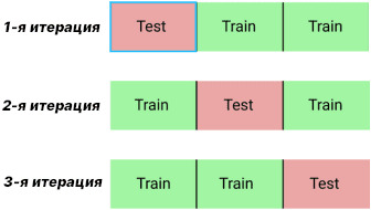
Кросс-валидация (N=3) В PySpark кросс-валидация реализуется через CrossValidator. В нем нам нужно указать три аргумента: estimator — модель Machine Learning, в нашем случае линейная регрессия; estimatorParamMaps — алгоритм оптимизации гиперпараметров, в нашем случае Grid Search; evaluator — метрика качества, в нашем случае RegressionEvaluator. Также можно указать в аргументах numFolds — количество блоков N (по умолчанию их 3). После указания значений этих аргументов вызывается метод fit для выполнения кросс-валидации. В Python это выглядит следующим образом: cv = CrossValidator(estimator=lin_reg, estimatorParamMaps=grid_search, evaluator=evaluator) cv_model = cv.fit(train)

Результаты кросс-валидации

Мы можем посмотреть модель с теми гиперпараметрами, которые показали наибольшую эффективность или, если быть точнее, наименьшее значение функции потерь. Для этого есть атрибут bestModel, который хранит информацию о лучшей модели. Мы можем посмотреть, например, на среднюю абсолютную ошибку: cv_model.bestModel.summary.meanAbsoluteError # 145260.09296909513 А также извлечь параметры этой модели. Нас больше интересует параметры регуляризации: cv_model.bestModel.extractParamMap() # { Param(parent='LinearRegression_b64ded0857c9', name='elasticNetParam', doc='the ElasticNet mixing parameter, in range [0, 1]. For alpha = 0, the penalty is an L2 penalty. For alpha = 1, it is an L1 penalty'): 1.0, Param(parent='LinearRegression_b64ded0857c9', name='regParam', doc='regularization parameter (>= 0)'): 0.1, } Как видим, лучшая модель имеет гиперпараметр elasticNetParam равный 1, а regParam — 0.1. Значения этих параметров показывают, что лучшая модель использует L1-регуляризацию (regParam > 0, elasticNetParam=1). Больше подробностей о линейной регрессии, L1 и L2 регуляризации, алгоритмах подбора гиперпараметрах, а также о кросс-валидации в PySpark на примерах задач Data Science и Big Data вы узнаете на наших практических курсах по Apache Spark и Machine Learning в лицензированном учебном центре обучения и повышения квалификации разработчиков, менеджеров, архитекторов, инженеров, администраторов, Data Scientist’ов и аналитиков Big Data в Москве: Анализ данных с Apache Spark Введение в машинное обучение на Python Введение в нейронные сети на Python Смотреть расписание Записаться на курс Источники https://en.wikipedia.org/wiki/Residual_sum_of_squares Read the full article

#MachineLearning #PySpark #Python #Spark #МашинноеОбучение #обработкаданных

0 notes

mathematicianadda · 5 years ago

Text

Limit associated with a recursion, connection to normality of quadratic irrationals

I posted a popular question 5 months ago about the following recursion, see here.

If $z_n < 2y_n$ Then

$y_{n+1} = 4y_n - 2z_n$

$z_{n+1} = 2z_n + 3$

$d_{n+1}=1$

Else

$y_{n+1} = 4y_n$

$z_{n+1} = 2 z_n - 1$

$d_{n+1}=0$

Back then, I wrote:

The sequence $d_n$ represents the binary digits of some unknown number $x$, a number that depends on the initial conditions. It turns out that if $y_1=2,z_1=5$ then that number is $x=\sqrt{2}$.

Here I offer a full solution and a potential path to proving the normality of quadratic numbers. My question is about proving that my main result (below) is correct. It is backed by very strong empirical results involving computations with thousands of digits. By normality, I mean that 50% of the binary digits of $x$ are equal to 1. This is one of the most challenging unsolved mathematical conjectures of all times.

Below is a Perl script that does all the computations. It uses the Bignum library to perform exact arithmetic (computation of millions of binary digits for each number, using the formulas described here.) The variable called number in the code corresponds to $x$.

use strict; use bignum; my $y; my $z; my $u; my $v; my $k; my $c; my $even; my $counter; my $seed_y; my $seed_z; my $number; my $denominator; my $c1; my $c2; $counter=0; open(OUT2,">collatzr.txt"); # summary stats open(OUT,">coll2.txt"); # details and digits for each number for ($seed_y=1; $seed_y<=5; $seed_y++) { for ($seed_z=$seed_y; $seed_z<=10; $seed_z++) { $y=$seed_y; $z=$seed_z; $u=2*$y-$z; $v=2*$z+3; $number=0; $denominator=1; $c1=0; $c2=0; for ($k=1; $k<200; $k++) { # compute 200 digits if ($u>0) { $even=1; # digit equal to 1 $c1++; $y=4*$y-2*$z; $z=2*$z+3; $u=4*$u-$v; $v=2*$v+3; } else { $even=0; # digit equal to 0 $c2++; $y=4*$y; $z=2*$z-1; $u=4*$u+$v-2; $v=2*$v-5; } print OUT "$seed_y\t$seed_z\t$k\t$even\n"; $denominator=$denominator/2; $number=$number+$even*$denominator; $c=$z*$denominator; } $counter++; if ($counter%5 == 0) { print "$seed_y\t$seed_z\n"; select()->flush(); } print OUT2 "$seed_y\t$seed_z\t$c1\t$c2\t$c\t$number\n"; } } close(OUT); close(OUT2);

1. Main result

Let $$x = \sum_{k=0}^\infty \frac{d_k}{2^k}, \mbox{ with } d_0=0 \tag 1$$

Then, assuming $y_0, z_0$ are positive integers, we have:

$y_0=0 \Rightarrow x=0$

$z_0 = 2y_0 \Rightarrow x=\frac{1}{2}$

$z_0 < y_0 \Rightarrow x=1$

In all other cases (referred to as the standard case), $x$ is an irrational quadratic number solution of $2x^2 +(z_0-1)x -y_0=0$, more specifically:

$$x =\frac{-(z_0-1)+\sqrt{(z_0-1)^2+8y_0}}{4} \tag 2$$

My question

Can you prove the above result? It was obtained empirically.

2. Useful tips to answer my question

In the standard case, we have the following result (not proved yet): $$\lim_{n\rightarrow\infty}\frac{z_n}{2^n}=\sqrt{(z_0-1)^2 + 8y_0}.$$

Also, using $u_n=2y_n-z_n$ and $v_n = 2z_n+3$, the recurrence can be rewritten as:

If $u_n>0$ Then

$u_{n+1}=4u_n -v_n$

$v_{n+1} = 2v_n + 3$

$d_{n+1}=1$

Else

$u_{n+1}=4u_n + v_n-2$

$v_{n+1} = 2v_n-5$

$d_{n+1}=0$

Finally, $\mbox{mod}(v_n, 8) = 5$, that is, $(v_n - 5)/8$ is an integer. If $n>1$ we have:

$$d_n = \mbox{ mod}\Big(\frac{v_n-5}{8},2\Big).$$ This leads to the following simple reverse recurrence involving only one variable, allowing you to compute the digits of $x$ backward, starting with a large $n$ and moving backward down to $n=1$:

$$\mbox{If mod}\Big(\frac{v_{n}-5}{8}, 2\Big) = 1, \mbox{ then } v_{n-1}=\frac{v_{n}-3}{2}, d_{n}=1, \mbox{ else } v_{n-1}=\frac{v_{n}+5}{2}, d_{n} = 0.$$

The very tough problem, outlined in the next section, is to prove that each of these two outcomes is equally likely to occur, on average. This would indeed be true if each $v_n$ is arbitrary, but this is not the case here. Also, if for some large $n$, we have $d_n=1$, then a run of $R$ successive digits $d_{n-1},\dots,d_{n-R}$ all equal to zero can only go so far, unless $v_n$ is a very special number not leading to $x$ being irrational. Maybe $R=\lfloor 2\sqrt{n}\rfloor$ is an upper bound. This is something worth exploring.

Property of the reverse recurrence: If $\mbox{mod}(v_n,8)=5$ and $v_n > 5$, then the sequence $v_n, v_{n-1},\dots$ is strictly decreasing until it reaches $5$ and stays there permanently; also each term is congruent to $5$ modulo $8$. This is true whether or not $v_n$ was generated using our forward recurrence.

An interesting application of this property is as follows. Take an arbitrary number, say $x = \log 2$. Multiply by a large power of $2$, say $2^{30}$. Round the result to the closest integer congruent to $5$ modulo $8$, and let this be your $v_n$. In this case, $v_n =\lfloor 2^{30} \log 2 \rfloor$. Compute $v_{n-1}, v_{n-2}$ and so on, as well as the associated digits, using the reverse recurrence. Stop when you hit $5$. The digits in question are the first binary digits of $\log 2$ yielding the approximation $0.693147175\dots$ while the exact value is $0.693147180\dots$

A similar reverse recurrence is also available for the original system: If $\mbox{mod}(\frac{z_{n}-1}{4}, 2) = 1$, then $z_{n-1}=\frac{z_{n}-3}{2}$, $d_{n}=1$, else $z_{n-1}=\frac{z_{n}+1}{2}$, $d_{n} = 0$. We also have $\mbox{mod}(z_n,4)=1$.

3. Connection to normality of irrational quadratic numbers

This is not part of my question, just interesting, extra material for the curious reader, and to provide some background as to why I am interested in this recursion. Do not even try to solve my problem below: contrarily to the main result, this stuff is incredibly hard; it could keep you busy and depressed for many years.

Let $S_n$ denotes the number of binary digits $d_k$ of $x$, that are equal to 1, for $k=1,\cdots, n$. If irrational quadratic numbers were indeed normal as we all believe they are, then, there is an absolute constant $K$ (not depending on $x$), and for each $x$, there is a number $N(x)$ denoted as $N$, such that

$$\mbox{If } n > N, \mbox{ then } S_n - K\sqrt{n} \leq \frac{n}{2} \leq S_n + K\sqrt{n} \tag 3$$

This is a consequence of the Berry-Hessen theorem applied to Bernouilli variables. It is discussed in sections 1.1 and 1.2 in this article. The chart below shows $\frac{|2S_n - n|}{\sqrt{n}}$ on the Y-axis, with $n$ between 0 and 530,000 on the X-axis, for the case $y_0 = z_0 = 1$ leading to $x=\frac{\sqrt{2}}{2}$. It suggests (not a proof) that in this case, $N = 0$ and $K = 0.90$ might work.

To prove that $x$ has 50% of its binary digits equal to 1, a potential approach thus consists in proving that if the previous inequality is true for $n$ large enough, then it is also true for $n+1$, by looking at the worst case scenario for the potential distribution of the first $n$ binary digits of $x$, using the recurrence relation introduced at the beginning, or the backward recurrence.

Some of the numbers $x$ that I tested are approaching the 50% ratio in question rather slowly, for instance if $y_0=1, z_0=16$. Indeed, I am wondering if some of these quadratic irrationals, maybe a finite number of them, even though normal, do not satistfy $(3)$, but instead a weaker result, say with $\sqrt{n}$ replaced by $n^{3/4}$ or $\frac{\log n}{n}$. To the contrary, a very fast convergence, say $n^{1/4}$ or $\log n$ instead of $\sqrt{n}$ in $(3)$, would also mean, even though $x$ may be normal, that its digits are not distributed like i.i.d. Bernouilli$(\frac{1}{2})$ variables. The only way for this Bernouilli behavior to happen, is if the convergence to the 50% ratio occurs at the right speed, that is with $\sqrt{n}$ in inequality $(3)$. In other words, for a specific $x$, any asymptotic departure from $\sqrt{n}$ in $(3)$ would mean that its binary digits are not distributed in a purely random way. This "pure randomness" criterion is stronger than having 50% of the digits equal to 1. For instance, $x=\frac{2}{3}=0.10101010\dots$ (in base 2) has 50% of its digits equal to 1, but the term $O(\sqrt{n})$ in $(3)$ can be replaced by the optimum bound $O(1)$, and the digits look anything but random.

I am doing some simulations and testing at this moment, see for instance my recent question on CrossValidated, here.

from Hot Weekly Questions - Mathematics Stack Exchange from Blogger https://ift.tt/2vjd1OG

#Blogger

0 notes

craigbrownphd-blog-blog · 6 years ago

Text

Fresh from the Python Package Index

• tuneRs Package for tuning hyperparameters with resampling methods. tuneRs is a small package for tuning hyperparameters using resampling methods instead of normal crossvalidation. Estimating model accuracy using resampling methods is much quicker that using k-fold crossvalidation–although resampling tends to underestimate accuracy more that crossvalidation. Resampling underestimates accuracy in a *consistent* fashion, however, which still makes it valuable for tuning hyperparameters. Due to it’s consistency, choosing hyperparameters based on aggregated samples still gets within the neighborhood of maximal while being much, much faster. This is a package to help you get there. • vector-shortcuts Vector and linear algebra toolbelt for NumPy • chatboteora EORA – your personal bot • eeyore Monte Carlo methods for neural networks • heron-model Heron is a machine learning package for Python. The ‘heron’ package is a python library for using Gaussian Process Regression (GPR) to emulate functions which are expensive to It was originally built for producing a surrogate model for numerical relativity waveforms from binary black hole coalesences, but the code should be sufficiently general to allow other surrogate models to be built. In order to handle very large models, ‘heron’ can use the ‘george’_ python package to generate the underlying Gaussian Process, which can handle very large models thanks to its use of a hierarchical matrix inverter. • sms-tools tools for sound analysis/synthesis • testOpendataset SDK for the Open Image Dataset. • torch-tools A library of helpers to train, evaluate and visualize deep nets with PyTorch. • wordlike Generates pronounceable nonsense words using Markov chains. • FastBLEU This is a fast multithreaded C++ implementation of nltk BLEU. • labelseg label tool for semantic segmentation • LexData A tiny package for editing Lexemes on Wikidata. This is a small library to create bots, scripts and tools about Wikidata Lexemes. It’s philosophy is to have a transparent thin layer on top of the internal datastuctures enriched with convenient functions without hiding the power of the access to the internals. http://bit.ly/38YS76I

0 notes

ermiaseyob-blog · 8 years ago

Text

Machine Learning: Regression with stochastic volatility

I had gotten right now there by a long search that had gone from machine learning, to fast Kalman filtration system, to Bayesian conjugate thready regression, to representing concern in the covariance using an inverse Wishart prior, in order to it time-varying, and allowing heteroschedasticity. I was thinking whith my friends which paper had all the items of an algorithm I think is fitted to forecasting intraday returns via signals. The features I like about imachine learning and the algotithm: Analytic: does not require sampling which is very slow. Just runs on the couple of matrix multiplications. Online: updates parameter values each and every single timestep. Offline/batch learning algorithms are typically too slow to retrain at every timestep within a backtest, which forces one to make sacrifices. Multivariate: cannot do without this. Adaptable regression coefficients: signals are weighted higher or much more depending on recent performance. Entirely forgetful: every part is adaptive, unlike some learners that happen to be partially adaptive and partially sticky. Adaptive variance: common linear regression is biased if the inputs are heteroschedastic unless you reweight input factors by the inverse of their variance. Adaptive input correlations: just in case signals become collinear. Estimations prediction error: outputs the estimated variance of the conjecture so you can choose how much you would like to trust it. This price is interpretable unlike a number of the heuristic approaches to extracting assurance intervals from other learners.

Interpretable internals: every internal variable is understandable. Looking at the internals clearly explains what the model has learned. Uni- or multi-variate: specializes or perhaps generalizes naturally. The only adjustment required is to increase or perhaps decrease the number of parameters, the values don’t need to be transformed. 10 input variables happens to be well as 2 which will works as well as 1 . Interpretable parameters: parameters are always set based on a-priori expertise, not exclusively by crossvalidation. The author re-parameterized the unit to make it as intuitive as possible - the variables are basically exponential lower price factors. Minimal parameters: it has just the right number of parameters to constitute a useful family nonetheless no extra parameters which have been rarely useful or unintuitive. Objective priors: incorrect beginning values for internal parameters do not bias predictions for the long “burn-in” period. Emphasis on first-order effects: alpha is a first-order effect. Higher order results are nice but first is so hard to identify that they are not worth the additional parameters and wasted datapoints. Bayesian: with a Bayesian model you understand all the assumptions starting your model. To learn more about variance see this useful web portal.

0 notes

craigbrownphd · 6 years ago

Text

Fresh from the Python Package Index

0 notes

insightmedpub-blog · 6 years ago

Text

In silico Quantitative Structure Pharmacokinetic Relationship Modeling on Antidiabetic Drugs: Time to Reach Peak Plasma Concentration

An estimate of time to reach peak plasma concentration (tmax) is of paramount importance in estimating thr rate of absorption and efficacy of drugs to treat acute conditions viz. polyphasia, polydispia and fatigue to treat diabetes in patients. This study was conducted to develop Quantitative Structure Pharmacokinetic Relationship (QSPkR) for the prediction of tmax in human for congeneric series of seventeen antidiabetic drugs, using computer assisted Hansch approach. The QSPkR correlations were duly analyzed using a battery of apt statistical procedures and validated using leave-one-out (LOO) approach. Analysis of several hundreds of QSPkR correlations developed in this study revealed high degree of crossvalidated coefficients (Q2 ) using LOO method (p<0.005). The overall predictability for time to reach peak plasma concentration was found to be high (R2 =0.9325, F=30.41, S2 =0.1253, Q2 =0.8502, p<0.005). The value of tmax of all drugs was found to depend upon various constitutional, topological and electrostatic parameters. Logarithmic transformation of the tmax value resulted in increase in correlation coefficient (R2 =0.9751, F=65.19, S2 =0.0016, Q2 =0.9411, p<0.005).

Further details @ http://www.imedpub.com/

For more details @ http://www.imedpub.com/articles/in-silico-quantitative-structure-pharmacokinetic-relationship-modeling-on-antidiabetic-drugs-time-to-reach-peak-plasma-concentrati.pdf

#insight medical publishing #medical journals #free online medical journals #open access scientific research publisher

0 notes

jane-doe-coursera-blog · 7 years ago

Text

Course 4 - Week 1

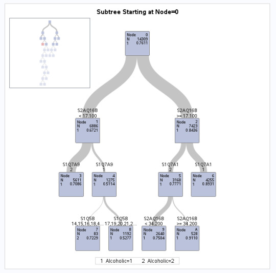
I built a decision tree for my binary categorical response variable “Alcoholic“. Because SAS tests for the occurrence of the lowest value the variable takes on, I coded Alcoholic=1 if the person is alcohol-dependent and Alcoholic=2 is the person is not. With this, the model event predicted is the presence of alcoholism and not its absence.

The output of the HPSPLIT procedure is presented above. We can see that the tree had 348 leaves before pruning and 15 leaves after pruning. There were 43,093 observations read from the data set and 14,309 thereof were used as these had valid data for the explanatory as well as the target variables.

The cost-complexity analysis shows the crossvalidated average standard error (ASE) for each number of leaves. The tree with 13 leaves has the lowest ASE. The final tree has splits for the age when a person first started drinking alcohol weekls (S2AQ16B) as a split node twice, whether the person is retired (S1Q7A9), the age at which the individuals had their first child (S1Q5B), whether they are employed full-time (S1Q7A1).

When we look at the confusion matrix, it becomes clear that the model correctly predicted 97% (error rate=0.03) of the Alcoholics, but only 13% (error rate=0.87) of the non-alcoholics. So we are more likely to correctly predict the presence of alcoholism rather than its absence.

There are some variables that are included in the variable importance training that were not selected as split nodes, such as age at first marriage, the race variables or drinking starting age. These are thus masked by other variables that were included as splits.

0 notes

incegna · 5 years ago

Photo

NLP is a field in machine learning with the ability of a computer to understand, analyze, manipulate, and potentially generate human language. https://www.incegna.com/post/natural-language-processing-nlp-for-machine-learning Check our Info : www.incegna.com Reg Link for Programs : http://www.incegna.com/contact-us Follow us on Facebook : www.facebook.com/INCEGNA/? Follow us on Instagram : https://www.instagram.com/_incegna/ For Queries : [email protected] #machinelearning,#nlp,#python,#analyzing,#NLTK,#conda,#Dataset,#numpy,#pandas,#Tokenization,#Stemming,#Lemmatizing,#Vectorizing,#ngrams,#Naivebayes,#crossvalidation https://www.instagram.com/p/B989dM_gf64/?igshid=utieudvip59r

#machinelearning #nlp #python #analyzing #nltk #conda #dataset #numpy #pandas #tokenization #stemming #lemmatizing #vectorizing #ngrams #naivebayes #crossvalidation

0 notes

deepak6446-blog · 6 years ago

Video

youtube

Machine learning - what is KFold cross-validation and why do i need to u...

#machine learning #artificial intelligence #kfold #crossvalidation sklearn

0 notes

engdashboard · 8 years ago

Text

Cross-Validation for Predictive Analytics Using R

Photo credits: http://ift.tt/2zEtqei Cross-Validation for Predictive Analytics Using Rhttp://ift.tt/1SLrR3g http://ift.tt/2zobx2i http://ift.tt/2zEk6GY http://ift.tt/2zobxzk http://ift.tt/2zEk7e0 VIDEOS

R-Session 5 - Statistical Learning - Resampling Methods

Hamed Hasheminia

https://www.youtube.com/watch?v=rGle0kv_hBc

DSO 530: LOOCV and k-fold CV in R

Abbass Al Sharif

https://www.youtube.com/watch?v=bRTIgv_UVxY

and more:

http://ift.tt/1L10TBw

crossValidation

Jeff Leek

https://www.youtube.com/watch?v=CmEqvD_ov2o&list=PLaRYai6fSpAqwRRYt6rVxKmCpN9tH26LX&index=1

https://www.youtube.com/playlist?list=PLaRYai6fSpAqwRRYt6rVxKmCpN9tH26LX

http://ift.tt/2zobGmm

via Blogger http://ift.tt/2xTADEU

0 notes

edeskar-dai-blog · 8 years ago

Text

Capstone project - Assignment 2

Draft of methods section

Description of sample

The data origins from a consultat company in Sweden. The roughness meausurement data consists of summer and winter measurements. Two lines in each driving direction, inner and outer wheelpath, has been monitored. The data has been processed by the company to IRI for every 0.1 m of the road section. The manual frost damage inventory was carried out at the same time as the winter roughness measurements. The used classification system defines the damages by a quantitaive scale 0-5, where 0 is no damage at all and 5 very severe. The damages included in the classification system are; roughness, cracks, block heave and culvert heave.

The three road sections are denoted A, B and C. Road A is 17700 m long. The observations is n=171890. Road B is 18980 m long. The observations is n= 170080. Road C is 12900 m long. The observations is n=170000.

Measures

The measures used in this and how these are managed in this study are:

The distance (DIST) is the the distance from the starting point of the road section.

The summer IRI measures are called (SUM_POS_SIDE) for the monitoring line of the inner wheelpath, (SUM_POS_CENTER) for the monitoring line of the outer wheelpat for the summer measurements in the positive driving direction. For the opposite direction the IRI measures are called (SUM_NEG_SIDE) and SUM_NEG_CENTER). The unit is quantitative (mm/m).

The corresponding measures for the winter survey are (WIN_POS_SIDE), (WIN_POS_CENTER), (WIN_NEG_SIDE), WIN_NEG_CENTER). The unit is quantitative (mm/m).

The frost damage inventory data has the following measures: the distance(DIST) in (m) starting from the same point as the IRI measures. The quantitative classification measures on the dummy scale 0-5; roughness (ROUGH), cracks (CRACK), block lift (BLOCK), culvert lift (CULVERT),

The data management will follow the the following procedure:

All data will be collected in one dataframe using (DIST) as key.

A number of computed IRI measures will be computed and tested as explanatory variables:

DELTA IRI = winter IRI - summer IRI

ABS(DELTA IRI) = ABS(winter IRI-summer IRI)

IRI_RATIO = winter IRI / summer IRI

The inventory data will be binned into the groups 0, 1, 2, 3, 4, 5. The original data containes additional coding that needs to be cleared out.

To compute IRI_ratio summer IRI data =0 mm/m needs to be replaced with 0.001 to avoid division by 0. Winter IRI will be limited to 50 mm/m to reduce monitoring errors. 50 mm/m is a very high value.

In the analysis boolean masking will be used to subset the datafram to isolate groups of different classifications.

Different lengths of roling means on IRI-data will be tested to investigate the effect of mismatching distance data.

Description of the statistical analysis

All analysis will be performed in Python 3.5.

At this stage the following statistical analysis are planned:

Descriptive statistics of all variables, including histograms and maybe also if possible statistical distribution tests.

Hypothesis 1:

There is a difference between classified roughness by the manual inventory and non-classified roughness (t-test)

Hypothesis 2:

There is a correlation bewteen the IRI-measures and the manual classified roughness (regression analysis).

Hypothesis 3:

It is possible to separate the different classes of each damage by IRI-measures. (t-test)

Hypothesis 4:

Other IRI-measures than the winter roughness are better suited to classify the damages. (k-cluster analysis).

For the linear regression the following assumptions will be checked

Normality - Residuals are normally distributed

Homoscedasticty - The variability in the response variable is the same at all levels of the explanaory variable.

Assume independence - check:

Multicollinearity

Outliers

If more variables are identified when analysing the data linear regression may be applied in order to rank the importance among the variables. This method is preferred prior k-cluster since in this case we have some physical understanding of the problem. Cross validiation will be applied on the lasso-regression analysis to evaluate the result. K-fold crossvalidation will be applied. In this case I think k= 10 is appropriate to test the robustness.

0 notes