#dataframe

[theinfectedbat]

Let's go to the basics then

[splicejunction]

If I start posting about my ocs you guys have to all pretend you can’t tell who they’re all based on. like i need you all to promise to pretend I’m capable of original thought

[govindhtech]

BigQuery DataFrame And Gretel Verify Synthetic Data Privacy

It looked at how combining Gretel with BigQuery DataFrame simplifies synthetic data production while maintaining data privacy in the useful guide to synthetic data generation with Gretel and BigQuery DataFrames. In summary, BigQuery DataFrame is a Python client for BigQuery that offers analysis pushed down to BigQuery using pandas-compatible APIs.

Gretel provides an extensive toolkit for creating synthetic data using state-of-the-art machine learning methods, such as large language models (LLMs). An seamless workflow is made possible by this integration, which makes it simple for users to move data from BigQuery to Gretel and return the created results to BigQuery.

The technical elements of creating synthetic data to spur AI/ML innovation are covered in detail in this tutorial, along with tips for maintaining high data quality, protecting privacy, and adhering to privacy laws. In Part 1, to de-identify the data from a BigQuery patient records table, and in Part 2, it create synthetic data to be saved back to BigQuery.

Setting the stage: Installation and configuration

With BigFrames already installed, you may begin by using BigQuery Studio as the notebook runtime. To presume you are acquainted with Pandas and have a Google Cloud project set up.

Step 1: Set up BigQuery DataFrame and the Gretel Python client.

Step 2: Set up BigFrames and the Gretel SDK: To use their services, you will want a Gretel API key. One is available on the Gretel console.

Part 1: De-identifying and processing data with Gretel Transform v2

De-identifying personally identifiable information (PII) is an essential initial step in data anonymization before creating synthetic data. For these and other data processing tasks, Gretel Transform v2 (Tv2) offers a strong and expandable framework.

Tv2 handles huge datasets efficiently by combining named entity recognition (NER) skills with sophisticated transformation algorithms. Tv2 is a flexible tool in the data preparation pipeline as it may be used for preprocessing, formatting, and data cleaning in addition to PII de-identification. Study up on Gretel Transform v2.

Step 1: Convert your BigQuery table into a BigFrames DataFrame.

Step 2: Work with Gretel to transform the data.

Part 2: Generating synthetic data with Navigator Fine Tuning (LLM-based)

Gretel Navigator Fine Tuning (NavFT) refines pre-trained models on your datasets to provide high-quality, domain-specific synthetic data. Important characteristics include:

Manages a variety of data formats, including time series, JSON, free text, category, and numerical.

Maintains intricate connections between rows and data kinds.

May provide significant novel patterns, which might enhance the performance of ML/AI tasks.

Combines privacy protection with data usefulness.

By utilizing the advantages of domain-specific pre-trained models, NavFT expands on Gretel Navigator’s capabilities and makes it possible to create synthetic data that captures the subtleties of your particular data, such as the distributions and correlations for numeric, categorical, and other column types.

Using the de-identified data from Part 1, it will refine a Gretel model in this example.

Step 1: Make a model better:

# Display the full report within this notebooktrain_results.report.display_in_notebook()

Step 2: Retrieve the Quality Report for Gretel Synthetic Data.

Step 3: Create synthetic data using the optimized model, assess the privacy and quality of the data, and then publish the results back to a BQ table.

A few things to note about the synthetic data:

Semantically accurate, the different modalities (free text, JSON structures) are completely synthetic and retained.

The data are grouped by patient during creation due to the group-by/order-by hyperparameters that were used during fine-tuning.

How to use BigQuery with Gretel

This technical manual offers a starting point for creating and using synthetic data using Gretel AI and BigQuery DataFrame. You may use the potential of synthetic data to improve your data science, analytics, and artificial intelligence development processes while maintaining data privacy and compliance by examining the Gretel documentation and using these examples.

Read more on Govindhtech.com

[vafion-vacational-rentals]

The Role of AI in Content Creation: ChatGPT, MidJourney, and Beyond

[exceltricks]

Python-Funktionen in Excel: Einfache Möglichkeiten zur Wortzählung

Auf dem YouTube-Kanal von Mr. Excel Bill Jelen wurde ein interessantes Video zu dem Thema Python-Funktionen in Excel veröffentlicht. Es geht in dem Video um die Anwendung einer benutzerdefinierten Python-Funktion zur Wortzählung. Vielleicht haben Sie sich auch schon gefragt, wie oft ein bestimmtes Wort in einem langen Text vorkommt. Diese Frage wird in dem Video sowohl in Excel als auch in Python…

[rajaniesh]

Exploring the Latest Features of Apache Spark 3.4 for Databricks Runtime

In the dynamic landscape of big data and analytics, staying at the forefront of technology is essential for organizations aiming to harness the full potential of their data-driven initiatives.

[pythonbaires]

Aprende a analizar datos con python!

En este curso aprenderás cómo analizar datos en Python usando matrices multidimensionales en numpy, a manipular DataFrames en pandas, a usar la biblioteca SciPy de rutinas matemáticas y a realizar aprendizaje automático usando scikit-learn. Comienza ya mismo! Pasarás de comprender los conceptos básicos de Python a explorar muchos tipos diferentes de datos a través de clases, laboratorios…

[the-bias-identifierrrr]

I am willing to accept a degree of variable repetition when you’ve clearly pieced a dataframe together from multiple sources.

But.

Having Year and Year.Code from the same dataframe, with the EXACT same values, RIGHT next to each other, is too much. Clean your data even SLIGHTLY before making it publicly available, I BEG of you

[techinfotrends]

Want to seamlessly combine your data? Learn the top 3 ways to merge Pandas DataFrames. Whether it's concatenation, merging on columns, or joining on index labels, these techniques will streamline your data analysis. https://bit.ly/3Y1GWG0

[hootyhoowoo]

Luo Binghe and his momma

[ID: Scum Villain sketches of Luo Binghe and his mother, the washerwoman, who is portrayed as a stout, older woman with her hair tied back into a small bun.

In image one, she frets over Luo Binghe with: "Aiyah - A'Luo, you need to eat more! No skipping meals, okay? The demon generals can wait. Too skinny..." In reply, Binghe abashedly bows and acquiesces, "Yes, A'niang..." / In image two, they are preparing dumplings together. Luo Binghe shows off how he folded his and asks, "Like this?" to which his mother nods and exclaims, "Perfect!" END ID.]

ID by @dataframe thank you!! <3

[splicejunction]

lev & annie dataframe crucially aren’t lab experiments but it’s close enough and I need material for the tag

[govindhtech]

Exploring BigQuery DataFrames and LLMs data production

Data processing and machine learning operations have been difficult to separate in big data analytics. Data engineers used Apache Spark for large-scale data processing in BigQuery, while data scientists used pandas and scikit-learn for machine learning. This disconnected approach caused inefficiencies, data duplication, and data insight delays.

At the same time, AI success depends on massive data. Thus, any firm must generate and handle synthetic data, which replicates real-world data. Algorithmically modelling production datasets or training ML algorithms like generative AI generate synthetic data. This synthetic data can simulate operational or production data for ML model training or mathematical model evaluation.

BigQuery DataFrames Solutions

BigQuery DataFrames unites data processing with machine learning on a scalable, cost-effective platform. This helps organizations expedite data-driven initiatives, boost teamwork, and maximize data potential. BigQuery DataFrames is an open-source Python package with pandas-like DataFrames and scikit-learn-like ML libraries for huge data.

It runs on BigQuery and Google Cloud storage and compute. Integrating with Google Cloud Functions allows compute extensibility, while Vertex AI delivers generative AI capabilities, including state-of-the-art models. BigQuey DataFrames can be utilized to build scalable AI applications due to their versatility.

BigQuery DataFrames lets you generate artificial data at scale and avoids concerns with transporting data beyond your ecosystem or using third-party solutions. When handling sensitive personal data, synthetic data protects privacy. It permits dataset sharing and collaboration without disclosing personal details.

Google Cloud can also apply analytical models in production. Testing and validation are safe with synthetic data. Simulate edge cases, outliers, and uncommon events that may not be in your dataset. Synthetic data also lets you model data warehouse schema or ETL process modifications before making them, eliminating costly errors and downtime.

Synthetic data generation with BigQuery DataFrames

Many applications require synthetic data generation:

Real data generation is costly and slow.

Unlike synthetic data, original data is governed by strict laws, restrictions, and oversight.

Simulations require larger data.

What is a data schema

Data schema

Let’s use BigQuery DataFrames and LLMs to produce synthetic data in BigQuery. Two primary stages and several substages comprise this process:

Code creation

Set the Schema and instruct LLM.

The user knows the expected data schema.

They understand data-generating programmes at a high degree.

They intend to build small-scale data generation code in a natural language (NL) prompt.

Add hints to the prompt to help LLM generate correct code.

Send LLM prompt and get code.

Executing code

Run the code as a remote function at the specified scale.

Post-process Data to desired form.

Library setup and initialization.

Start by installing, importing, and initializing BigQuery DataFrames.

Start with user-specified schema to generate synthetic data.

Provide high-level schema.

Consider generating demographic data with name, age, and gender using gender-inclusive Latin American names. The prompt states our aim. They also provide other information to help the LLM generate the proper code:

Use Faker, a popular Python fake data module, as a foundation.

Pandas DataFrame holds lesser data.

Generate code with LLM.

Note that they will produce code to construct 100 rows of the intended data before scaling it.

Run code

They gave LLMs all the guidance they needed and described the dataset structure in the preceding stage. The code is verified and executed here. This process is crucial since it involves humans and validates output.

Local code verification with a tiny sample

The prior stage’s code appears fine.

They would return to the prompt and update it and repeat the procedures if the created code hadn’t ran or Google wanted to fine-tune the data distribution.

The LLM prompt might include the created code and the issue to repair.

Deploy code as remote function

The data matches what they wanted, so Google may deploy the app as a remote function. Remote functions offer scalar transformation, thus Google can utilize an indicator (in this case integer) input and make a string output, which is the code’s serialized dataframe in json. Google Cloud must additionally mention external package dependencies, such as faker and pandas.

Scale data generation

Create one million synthetic data rows. An indicator dataframe with 1M/100 = 10K indicator rows can be initialized since our created code generates 100 rows every run. They can use the remote function to generate 100 synthetic data rows each indication row.

Flatten JSON

Each item in df[“json_data”] is a 100-record json serialized array. Use direct SQL to flatten that into one record per row.

The result_df DataFrame contains one million synthetic data rows suitable for usage or saving in a BigQuery database (using the to_gbq method). BigQuery, Vertex AI, Cloud Functions, Cloud Run, Cloud Build, and Artefact Registry fees are involved. BigQuery DataFrames pricing details. BigQuery jobs utilized ~276K slot milliseconds and processed ~62MB bytes.

Creating synthetic data from a table structure

A schema can generate synthetic data, as seen in the preceding step. Synthetic data for an existing table is possible. You may be copying the production dataset for development. The goal is to ensure data distribution and schema similarity. This requires creating the LLM prompt from the table’s column names, types, and descriptions. The prompt could also include data profiling metrics derived from the table’s data, such as:

Any numeric column distribution. DataFrame.describe returns column statistics.

Any suggestions for string or date/time column data format. Use DataFrame.sample or Series.sample.

Any tips on unique categorical column values. You can use Series.unique.

Existing dimension table fact table generation

They could create a synthetic fact table for a dimension table and join it back. If your usersTable has schema (userId, userName, age, gender), you can construct a transactionsTable with schema (userId, transactionDate, transactionAmount) where userId is the key relationship. To accomplish this, take these steps:

Create LLM prompt to produce schema data (transactionDate, transactionAmount).

(Optional) In the prompt, tell the algorithm to generate a random number of rows between 0 and 100 instead of 100 to give fact data a more natural distribution. You need adjust batch_size to 50 (assuming symmetrical distribution). Due to unpredictability, the final data may differ from the desired_num_rows.

Replace the schema range with userId from the usersTable to initialise the indicator dataframe.

As with the given schema, run the LLM-generated code remote function on the indicator dataframe.

Select userId and (transactionDate, transactionAmount) in final result.

Conclusions and resources

This example used BigQuery DataFrames to generate synthetic data, essential in today’s AI world. Synthetic data is a good alternative for training machine learning models and testing systems due to data privacy concerns and the necessity for big datasets. BigQuery DataFrames integrates easily with your data warehouse, Vertex AI, and the advanced Gemini model. This lets you generate data in your data warehouse without third-party solutions or data transfer.

Google Cloud demonstrated BigQuery DataFrames and LLMs synthetic data generation step-by-step. This involves:

Set the data format and use natural language prompts to tell the LLM to generate code.

Code execution: Scaling the code as a remote function to generate massive amounts of synthetic data.

Get the full Colab Enterprise notebook source code here.

Google also offered three ways to use their technique to demonstrate its versatility:

From user-specified schema, generate data: Ideal for pricey data production or rigorous governance.

Generate data from a table schema: Useful for production-like development datasets.

Create a dimension table fact table: Allows entity-linked synthetic transactional data creation.

BigQuery DataFrames and LLMs may easily generate synthetic data, alleviating data privacy concerns and boosting AI development.

Read more on Govindhtech.com

[vafion-vacational-rentals]

A Deep Dive into Rust: The Fastest-Growing Programming Language

Rust has rapidly emerged as one of the most popular programming languages in the developer community. Known for its performance, safety, and concurrency, Rust has earned the title of the “most loved” language in Stack Overflow’s Developer Survey for several years in a row. In this blog, we’ll explore the reasons behind Rust’s meteoric rise, its key features, benefits, and how it is being used in systems programming and beyond.

Why Rust is Gaining Popularity

1. Memory Safety Without Garbage Collection:

   – One of Rust’s most celebrated features is its ability to ensure memory safety without the need for a garbage collector (GC). In languages like C and C++, manual memory management often leads to issues like dangling pointers, buffer overflows, and memory leaks. Rust, however, uses a unique ownership system that ensures memory safety at compile time, preventing these common bugs.

2. Performance Comparable to C and C++:

   – Rust is a systems programming language designed to provide the performance of C and C++ while offering a more modern and safer syntax. It compiles to native code, which allows it to run as fast as traditionally low-level languages. This makes Rust an excellent choice for performance-critical applications like game engines, operating systems, and embedded systems.

3. Concurrency Without Data Races:

   – Concurrency is a key aspect of modern programming, and Rust excels in this area. It guarantees thread safety by preventing data races at compile time. Rust’s ownership model ensures that only one thread can mutate data at any given time, eliminating a whole class of concurrency bugs that plague other languages.

4. A Thriving Ecosystem and Strong Community Support:

   – Rust’s ecosystem has grown rapidly, with a rich set of libraries (crates) available through the Cargo package manager. The Rust community is also known for being welcoming and supportive, making it easier for new developers to learn and adopt the language.

5. Adoption by Major Companies:

   – Many tech giants have started adopting Rust in their codebases. For example, Mozilla (the creators of Rust), Dropbox, Cloudflare, and Microsoft have used Rust to improve performance and security in their products. This real-world adoption showcases Rust’s viability in production environments.

Key Features of Rust

1. Ownership and Borrowing:

   – Rust’s ownership model is its most distinctive feature. Each value in Rust has a single owner, and when the owner goes out of scope, the value is automatically deallocated. This ensures that memory is safely and efficiently managed without the need for garbage collection.

2. Pattern Matching:

   – Rust’s pattern matching is powerful and flexible, allowing developers to handle complex data structures with ease. It is particularly useful in control flow structures like `match` statements, which can destructure enums and other types.

3. Macros:

   – Rust’s macro system allows developers to write code that writes other code (metaprogramming). This can be used to reduce boilerplate, generate code based on patterns, and create domain-specific languages (DSLs) within Rust.

4. Cargo and Crates.io:

   – Cargo is Rust’s build system and package manager, making it easy to manage dependencies, run tests, and build projects. Crates.io is the central repository for Rust libraries, fostering a rich ecosystem of reusable code.

5. Error Handling:

   – Rust takes a pragmatic approach to error handling, encouraging the use of `Result` and `Option` types rather than exceptions. This makes it easier to write robust code that gracefully handles potential failures.

Benefits of Using Rust

1. Safety:

   – Rust’s strict compile-time checks ensure that code is memory-safe and free from common bugs like null pointer dereferencing, buffer overflows, and data races. This leads to more reliable and secure software.

2. Performance:

   – Without the overhead of garbage collection and with fine-grained control over memory usage, Rust can achieve performance on par with C and C++. This makes it suitable for performance-critical applications.

3. Productivity:

   – Despite its focus on safety and performance, Rust is designed to be ergonomic and developer-friendly. Features like pattern matching, powerful enums, and expressive error handling make it easier to write clear and concise code.

4. Concurrency:

   – Rust’s approach to concurrency ensures that code is free from data races, making it easier to write safe concurrent code. This is increasingly important in a world where multi-core processors are the norm.

5. Modern Tooling:

   – Rust’s tooling, particularly Cargo, simplifies the development process by handling dependency management, testing, and building. This allows developers to focus more on writing code and less on managing their development environment.

Use Cases of Rust in Systems Programming and Beyond

1. Operating Systems:

   – Rust’s performance and safety make it an excellent choice for developing operating systems. For example, Redox OS is a modern operating system written entirely in Rust. Its design leverages Rust’s features to create a secure and reliable OS from the ground up.

2. Web Assembly:

   – Rust has strong support for WebAssembly (Wasm), allowing developers to write high-performance code that runs in the browser. This opens up possibilities for web applications that require intensive computations, such as games or image processing tools.

3. Embedded Systems:

   – Rust’s low-level control over hardware makes it ideal for embedded systems development. It allows developers to write safe, concurrent code that runs on resource-constrained devices, such as microcontrollers or IoT devices.

4. Command-Line Tools:

   – Rust is popular for building command-line tools due to its speed, safety, and ease of cross-compilation. Tools like ripgrep (a fast search tool) and exa (a modern replacement for `ls`) showcase Rust’s capabilities in this domain.

5. Networking:

   – Rust’s safety and performance characteristics are particularly beneficial in networking, where reliability and speed are crucial. Projects like Tokio (an asynchronous runtime for Rust) and Actix (a powerful actor framework) have made Rust a popular choice for developing network services and applications.

6. Game Development:

   – Rust is also gaining traction in game development, with game engines like Amethyst and Bevy being developed in Rust. The language’s focus on performance and safety is particularly appealing for game developers who need to manage complex state and real-time computations.

Conclusion

Rust’s rapid rise in popularity is a testament to its unique combination of safety, performance, and modern programming features. Whether you’re building an operating system, a web application, or a command-line tool, Rust offers a powerful set of tools that can help you write efficient and reliable software. As more developers and companies adopt Rust, its ecosystem will continue to grow, making it an even more compelling choice for a wide range of applications. If you haven’t tried Rust yet, now might be the perfect time to dive in and experience what this fast-growing language has to offer. Visit :- https://www.vafion.com/blog/deep-dive-rust-fastest-growing-programming-language/

For more details contact info@vafion.com

Follow us on Social media  : Twitter |  Facebook | Instagram | Linkedin

[detrasdeldataset]

Explorando los Datos: Un Análisis Profundo sobre la Relación entre Alcoholismo y Trastornos de Ansiedad

Hoy continuaremos nuestra exploración en la investigación sobre la propensión al alcoholismo y su correlación con los trastornos de ansiedad. Como siguiente paso, nos sumergiremos en un análisis exploratorio de los datos obtenidos del estudio NESARC.

Dada la magnitud del conjunto de datos, nos enfrentamos a un desafío inicial debido a su considerable tamaño. Al cargar el archivo como un dataframe, notamos un consumo significativo de memoria, lo que podría potencialmente ralentizar la ejecución del código.

Para optimizar nuestra investigación, decidimos conservar únicamente las variables relevantes para nuestro estudio, las cuales se detallan en el libro de códigos.

LIBRO DE CÓDIGO.pdf

Durante este proceso, identificamos que algunas columnas no se importaron con el tipo de dato correcto. Por ejemplo, variables como 'S2AQ11', 'S3AQ2A1', y 'S3AQ3A1R', que representan el número de tragos tolerados sin sentirse intoxicado, la edad de inicio del consumo de tabaco, y la duración en horas desde la última vez que se consumió tabaco, respectivamente, deberían ser de tipo numérico, sin embargo, se detectaron como tipo 'objeto'. Del mismo modo, una lista de aproximadamente 32 variables que deberían ser categóricas también se identificó erróneamente como tipo 'objeto'.

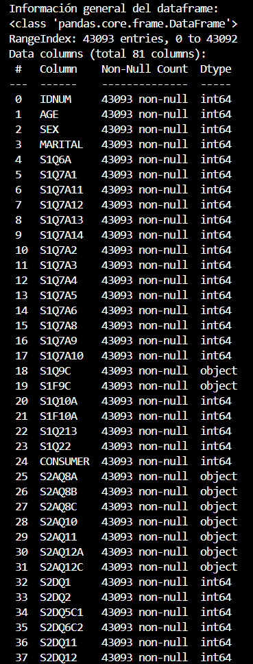
A continuación se presenta la salida en consola del método pandas.info() después de filtrar el dataframe original.

Durante la corrección del tipo de dato, además, reemplazamos las entradas que contenían espacios en blanco con valores NaN de la biblioteca NumPy, lo que permite a Python reconocer adecuadamente los valores faltantes.

A continuación se presenta la salida en consola del método pandas.info() después de corregir el tipo de dato para cada columna del dataframe:

Es importante destacar que, al realizar estos ajustes, logramos reducir significativamente el uso de memoria del dataframe. Cuando filtramos las columnas, conseguimos reducir el uso de memoria de 989.6MB a solo 26.6MB. Además, al dejar el dataframe con los tipos de columnas correctos, también conseguimos reducir el uso de memoria, quedando solamente 5.6MB. Esta reducción en el uso de memoria es crucial, ya que permite un procesamiento más eficiente de los datos y mejora el rendimiento del análisis exploratorio.

Con el dataframe corregido y cada columna ahora con su tipo de dato correcto, procedimos con el análisis exploratorio de los datos. Dado que contamos con un total de 81 variables, para una mejor comprensión de la estructura del conjunto de datos, decidimos presentar de manera ilustrativa la frecuencia de las variables de Edad, Sexo y Estado Civil.

Observamos que en el estudio hay más mujeres que hombres y el tipo de estado civil más común es el de Casado.

Posteriormente, analizamos el número de valores faltantes y el número de valores únicos por columna.

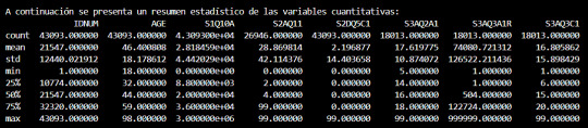
Por último, presentamos un resumen estadístico de las variables cuantitativas, lo que nos permite obtener una comprensión más profunda del comportamiento de los datos en nuestra muestra.

Con los datos limpios y un análisis exploratorio detallado en marcha, estamos en un punto crucial de nuestra investigación sobre la relación entre el alcoholismo y los trastornos de ansiedad. Esta optimización en el uso de memoria y la corrección de los tipos de datos nos permiten ahora adentrarnos aún más en el análisis de estos datos fundamentales.

Próximamente, estaremos explorando patrones y tendencias en los datos que podrían arrojar luz sobre la compleja interacción entre el alcoholismo y los trastornos de ansiedad. Manténgase atento para descubrir cómo estos hallazgos podrían informar no solo nuestra comprensión científica, sino también las posibles intervenciones y políticas para abordar estos desafíos de salud mental.

También puedes consultar el código utilizado aquí:

analisisexploratorio.py

Y descargar el dataset con el que estamos trabajando aquí:

nesarc_pds.csv

[exceltricks]

Python in Excel: Neue Dimension für Datenanalyse und Automatisierung

Liebe Excel-Enthusiasten, in meinem heutigen Blogbeitrag möchte ich Ihnen eine aufregende Neuerung in Microsoft Excel vorstellen, die das Potenzial hat, die Art und Weise, wie Sie Daten analysieren und automatisieren, grundlegend zu verändern. Es handelt sich um die Integration von Python in Excel, die nun im Beta-Kanal von Office 365 verfügbar ist. Excel hat in der Vergangenheit viele Updates…