#isomorphism theorems

[i-iii-iii-vii]

[the-autistic-introvert]

i think the coolest thing about being knowledgeable in something is that you get to have favourites (that other people may not understand). like how math people have their favourite theorems and geoguessr players have favourite poles. its like a secret exclusive group that most people just dont get to see

[michaelrotonal]

math people be like "if the group has a prime order then by Lagrange's Theorem every subgroup is either the trivial group or the whole group. that means every element other than the identity is a generator of the whole group, which means the group is cyclic. there's only one cyclic group of any order up to isomorphism so there is only one group of each prime order up to isomorphism" and other math people be like "yeah of course that's trivial"

[lipshits-continuous]

A Short Intro to Category Theory

A common theme in mathematics is to study certain objects and the maps between that preserve the specific structure of said objects. For example, linear algebra is the study of vector spaces and linear maps. Often we have that the identity maps are structure preserving and the composition of maps is also structure preserving. In the case of vector spaces, the identity map is a linear map and the composition of linear maps is again a linear map. Category theory generalises and axiomatises this common way of studying mathematical objects.

I'll introduce the notion of a category as well as the notion of a functor, which is another very important and ubiquitous notion in category theory. And I will finish with a very powerful result involving functors and isomorphisms!

Definition 1:

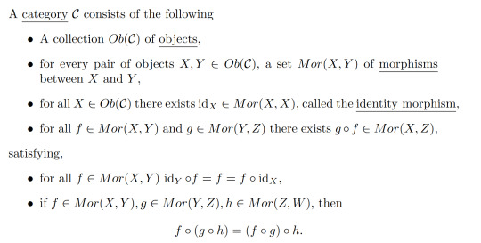
We call the last property the associative property.

Here are some examples:

Examples 2:

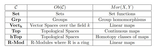
Note that whilst all of these examples are built from sets and set functions, we can have other kinds of objects and morphisms. However the most common categories are those built from Set.

Functors:

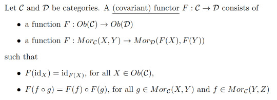
In the spirit of category theory being the study of objects and their morphisms, we want to define some kind of map between categories. It turns out that these are very powerful and show up everywhere in pure maths. Naturally, we want a functor to map objects to objects and morphisms to morphisms in a way that respects identity morphisms and our associative property.

Definition 3:

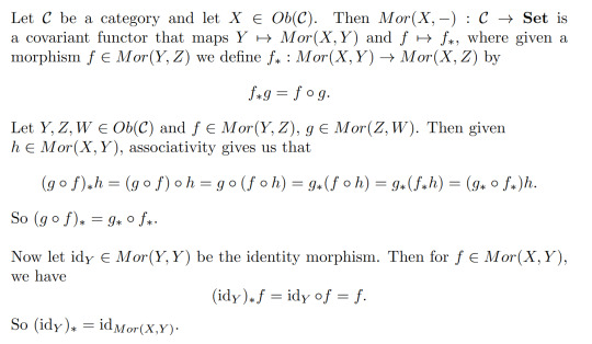
Example 4:

For those familiar with a some topology, the fundamental group is another exmaple of a covariant functor from the category of based spaces and based maps to Grp.

We also have another kind of functor:

Defintion 5:

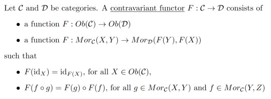
It may seem a bit odd to introduce at first since all we've done is swap the directions of the morphisms, but it turns out that contravariant functors show up a lot!

This example requires a little bit of knowledge of linear algebra.

Example 6:

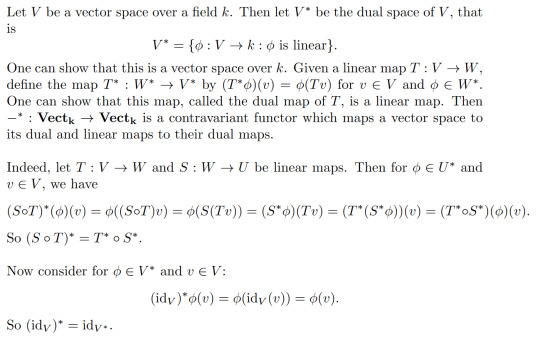
In fact, this is somewhat related to example 5! We can produce a contravariant functor Mor(-,X) is a similar way. For V and W vector spaces over k, we have that Mor(V,W) is a vector space over k. In particular, V*=Mor(V,k). So really this -* functor is just Mor(-,k)!

Isomorphisms

Here we generalise the familiar notion of isomorphisms of any algebraic structure!

Definition 7:

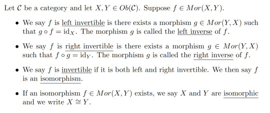
For a category of algebraic objects like Vectₖ, isomorphism are exactly the same as isomorphisms defined the typical way. In Top the isomorphisms are homeomorphisms. In Set the isomorphisms are bijective maps.

Remark:

So if f is invertible, we call it's right (or left) inverse, g, the inverse of f.

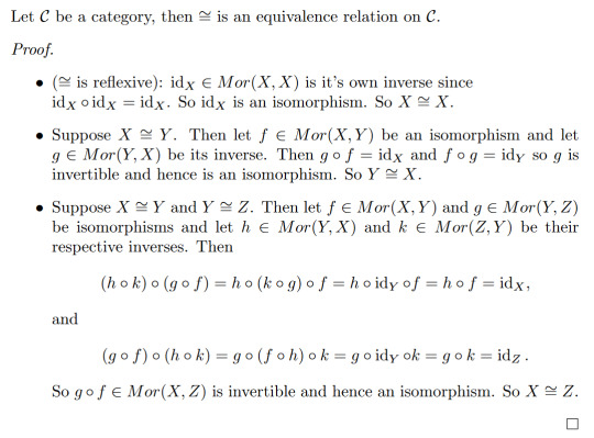
Isomorphisms give us a way to say when two objects of a category are "the same". More formally, being isomorphic defines an equivalence relation.

Lemma 8:

A natural question one might as is how do functors interact with isomorphisms? The answer is the very important result I hinted at in the intro!

Theorem 9:

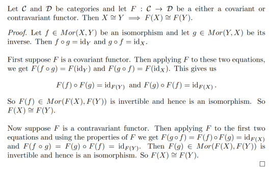
Remark: In general, the converse is not true. That is F(X) isomorphic to F(Y) does not imply X is isomorphic to Y. An example of this is the fundamental groups of both S² and ℝ² are isomorphic to the trivial group but these spaces are not homeomorphic.

Taking the negation of Theorem 9 gives us a very powerful result:

Corollary 10:

This means that if we can find a functor such that F(X) and F(Y) aren't isomorphic, we know that X and Y are not isomorphic. This is of particular importance in algebraic topology where we construct functors from Top or hTop to a category of a given algebraic structure. This gives us some very powerful topological invariants for telling when two spaces aren't homeomorphic or homotopy equivalent. (In fact, this is where category theory originated from!)

[m---a---x]

Welcome to the premier of One-Picture-Proof!

This is either going to be the first installment of a long running series or something I will never do again. (We'll see, don't know yet.)

Like the name suggests each iteration will showcase a theorem with its proof, all in one picture. I will provide preliminaries and definitions, as well as some execises so you can test your understanding. (Answers will be provided below the break.)

The goal is to ease people with some basic knowledge in mathematics into set theory, and its categorical approach specifically. While many of the theorems in this series will apply to topos theory in general, our main interest will be the topos Set. I will assume you are aware of the notations of commutative diagrams and some terminology. You will find each post to be very information dense, don't feel discouraged if you need some time on each diagram. When you have internalized everything mentioned in this post you have completed weeks worth of study from a variety of undergrad and grad courses. Try to work through the proof arrow by arrow, try out specific examples and it will become clear in retrospect.

Please feel free to submit your solutions and ask questions, I will try to clear up missunderstandings and it will help me designing further illustrations. (Of course you can just cheat, but where's the fun in that. Noone's here to judge you!)

Preliminaries and Definitions:

B^A is the exponential object, which contains all morphisms A→B. I comes equipped with the morphism eval. : A×(B^A)→B which can be thought of as evaluating an input-morphism pair (a,f)↦f(a).

The natural isomorphism curry sends a morphism X×A→B to the morphism X→B^A that partially evaluates it. (1×A≃A)

φ is just some morphism A→B^A.

Δ is the diagonal, which maps a↦(a,a).

1 is the terminal object, you can think of it as a single-point set.

We will start out with some introductory theorem, which many of you may already be familiar with. Here it is again, so you don't have to scroll all the way up:

Exercises:

What is the statement of the theorem?

Work through the proof, follow the arrows in the diagram, understand how it is composed.

What is the more popular name for this technique?

What are some applications of it? Work through those corollaries in the diagram.

Can the theorem be modified for epimorphisms? Why or why not?

For the advanced: What is the precise requirement on the category, such that we can perform this proof?

For the advanced: Can you alter the proof to lessen this requirement?

Bonus question: Can you see the Sicko face? Can you unsee it now?

Expand to see the solutions:

Solutions:

This is Lawvere's Fixed-Point Theorem. It states that, if there is a point-surjective morphism φ:A→B^A, then every endomorphism on B has a fixed point.

Good job! Nothing else to say here.

This is most commonly known as diagonalization, though many corollaries carry their own name. Usually it is stated in its contraposition: Given a fixed-point-less endomorphism on B there is no surjective morphism A→B^A.

Most famous is certainly Cantor's Diagonalization, which introduced the technique and founded the field of set theory. For this we work in the category of sets where morphisms are functions. Let A=ℕ and B=2={0,1}. Now the function 2→2, 0↦1, 1↦0 witnesses that there can not be a surjection ℕ→2^ℕ, and thus there is more than one infinite cardinal. Similarly it is also the prototypiacal proof of incompletness arguments, such as Gödels Incompleteness Theorem when applied to a Gödel-numbering, the Halting Problem when we enumerate all programs (more generally Rice's Theorem), Russells Paradox, the Liar Paradox and Tarski's Non-Defineability of Truth when we enumerate definable formulas or Curry's Paradox which shows lambda calculus is incompatible with the implication symbol (minimal logic) as well as many many more. As in the proof for Curry's Paradox it can be used to construct a fixed-point combinator. It also is the basis for forcing but this will be discussed in detail at a later date.

If we were to replace point-surjective with epimorphism the theorem would no longer hold for general categories. (Of course in Set the epimorphisms are exactly the surjective functions.) The standard counterexample is somewhat technical and uses an epimorphism ℕ→S^ℕ in the category of compactly generated Hausdorff spaces. This either made it very obvious to you or not at all. Either way, don't linger on this for too long. (Maybe in future installments we will talk about Polish spaces, then you may want to look at this again.) If you really want to you can read more in the nLab page mentioned below.

This proof requires our category to be cartesian closed. This means that it has all finite products and gives us some "meta knowledge", called closed monoidal structure, to work with exponentials.

Yanofsky's theorem is a slight generalization. It combines our proof steps where we use the closed monoidal structure such that we only use finite products by pre-evaluating everything. But this in turn requires us to introduce a corresponding technicallity to the statement of the theorem which makes working with it much more cumbersome. So it is worth keeping in the back of your mind that it exists, but usually you want to be working with Lawvere's version.

Yes you can. No, you will never be able to look at this diagram the same way again.

We see that Lawvere's Theorem forms the foundation of foundational mathematics and logic, appears everywhere and is (imo) its most important theorem. Hence why I thought it a good pick to kick of this series.

If you want to read more, the nLab page expands on some of the only tangentially mentioned topics, but in my opinion this suprisingly beginner friendly paper by Yanofsky is the best way to read about the topic.

[catgirl-lucy]

Axiom of Choice

Hiiiiii! Today, I'll explain what the axiom of choice (AC) is, and I'll show some statements (Zorn's lemma & the well-ordering principle) and show that they're equivalent to AC. I'll work in ZF.

First, the axiom of choice:

Given a family X of non-empty sets, there is a function f ∈ ΠX that maps every set A ∈ X to an element f(a) ∈ A.

Such a function is called a choice function for X. The set of choice functions on X is written as ΠX, which you can see as the product of all sets in X. x ∈ y is used to denote that x is a member of y.

If X is a finite set, then the above statement is provable. I'd always encourage the readers to prove these statements themselves. Since this is the first theorem of the day, I'll also give a proof:

[Theorem] If X is a finite family of non-empty sets, then there is a choice function f ∈ ΠX for X.

[Proof] Let X = {A₁..Aₙ}. We'll use induction on k. Assume n = 0, the empty function is a choice function for X. Suppose n = m + 1 and suppose the above statement holds for all sets of cardinality k (this assumption is called the induction hypothesis or IH). Let g be a choice function for {A₁..Aₘ}, which exists by IH. Let a ∈ Aₙ, which exists as Aₙ is non-empty by assumption. Define f ∈ Π{A₁..Aₙ} as follows: for 1 ≤ k ≤ m, we have f(Aₖ) = g(Aₖ), and otherwise, f(Aₙ) = a. ∎

So AC holds for finite sets, but there are sets for which it's not clear if AC holds. For example, ℝ/ℚ: this is the set of all sets [x] of real numbers for real x such that y ∈ [x] iff x - y is a rational number (note that [x] = [y] iff x - y ∈ ℚ). It thus partitions the real numbers into sets of reals that are a rational distance apart. A choice function for this set is a function f ∈ Πℝ/ℚ that maps every set of real numbers to some real number. You can try to construct such a choice function, but I don't think it'd work.

Most mathematicians assume that the axiom of choice holds, and thus that there is a function f: ℝ/ℚ → ℝ that maps every set [x] to some y ∈ [x].

There are many statements that are known to be equivalent to AC, one of them is the well-ordering principle:

Given a set A, there is a ≤ on A.

A well-order on A is a binary relation ≤ on A such that:

≤ is reflexive: x ≤ x for all x ∈ A.

≤ is transitive: if x ≤ y and y ≤ z, then x ≤ z, for all x,y,z ∈ A.

≤ is antisymmetric: if x ≤ y and y ≤ x, then x = y, for all x,y ∈ A.

≤ is total: x ≤ y or y ≤ x for all x,y ∈ A.

≤ is well-founded: for all non-empty subsets S ⊂ A of A, there is some minimum element x ∈ S, i.e. an element such that, for all y ∈ S, if y ≤ x, then x = y.

Axioms 1-2 describe a pre-order, 1-3 describe a partial order and 1-4 are for linear/total orders.

Proving that AC implies the well-ordering principle requires a technique called transfinite induction. The statement of transfinite induction is as follows:

For a non-empty set of ordinals S, there is some minimal element α ∈ S.

An ordinal is the order-type of a well-order. Given two ordered sets (A,≤A) and (B,≤B), they are said to have the same order-type iff there exists an isomorphism f: (A,≤A) → (B,≤B), i.e. a bijection from A to B such that, for all x,y ∈ A, x ≤A y holds iff f(x) ≤B f(y) holds. Thus, they have the same order-type if they have the same structure.

Order types can be ordered by a relation that I'll denote as ≼. For order-types α = ot(A,≤A) and β = ot(B,≤B) (ot(X,≤X) is the order-type of (X,≤X)), we have α ≼ β iff there exists an injection f: A → B such that, for all x,y ∈ A, x ≤A y holds iff f(x) ≤B f(y) holds. This means that α is “contained” in β. I'll use α ≺ β for α ≼ β ∧ ¬β ≼ α.

≼ is a pre-order on order-types in general: it is reflexive and transitive, but not antisymmetric, total or well-founded. However, if we restrict ≼ to only ordinals (thus, order-types of well-orders), then we get that ≼ is antisymmetric, total and well-founded, and thus a well-order.

A proof of this is left as an exercise to the reader.

The class of all ordinals is often denoted as Ord or On. I'll use Ord in this blog-post.

Functions can also be defined with transfinite induction: if f is a function with domain Ord, then we can define f(α) with respect to earlier values of f, i.e. f(β) for β < α. Here is an example of how we could use that: f(α) = f[α] ∪ {f[α]}, where f[α] = {f(β) | β < α} is the set of f applied to β for β < α. For an ordinal α, this gives us the von Neumann representation of α! :3

If we try to use induction to define functions on orders that are not well founded, it won't work: let f: ℤ → {-1,1} be a function defined as f(x) = -f(x-1). This definition does not define a unique function, f(x) could be (-1)^x, but it could also be -(-1)^x. Only with well-founded orders, f is guaranteed to be unique.

I'll use von Neumann ordinals from now on, as they're easy to work with. A von Neumann ordinal is the set of all previous ordinals, for example, 2 = {0,1} and ω = {0,1,2,3,...}.

Now that we know how transfinite induction works, we can show that AC implies the well ordering principle. Given a set A, we want to show there is a well-order ≺ on A. We can do this by defining bijective function f: α → A from some ordinal α to A. If we have such a bijection, we can define f(α) ≺ f(β) iff α < β, and ≺ then forms a well-order on A.

So, how do we define this bijection f: α → A? Well, suppose we already have a part of this bijection, g: β → A for some β < α. Since g is only partially complete, it isn't surjective, thus there is still some x ∈ A \ g[A], i.e. some x that has not been mapped to. We don't really have a good way of finding this x, so we need to use the axiom of choice.

We can take A \ {∅}, the set of all non-empty subsets of A. Let c be a choice function for A \ {∅}. Then, c(A \ g[A]) gives us some x ∈ A \ g[A].

Now, we can define f: α → A with transfinite induction. f(β) = c(A \ f[β]) as long as A \ f[β] isn't empty. If A \ f[β] is empty, then we set α := β. We can now use this bijection to show a well-order on A exists.

The converse direction, that the well-ordering lemma implies AC, is left as an exercise for the reader. Hint: infinite cardinal sums, which I've talked about in my previous blog-post, might help you with this!

Here is some terminology of partial orders, which will be useful for Zorn's lemma:

A partial ordered set, or poset, is a structure (X,≤) with a set X and a partial order ≤ (a partial order is reflexive, transitive and antisymmetric)

For two elements a,b ∈ X, a and b are comparable if a ≤ b or b ≤ a, they are incomparable, written a ⊥ b, if they are not comparable

A maximal element is some a ∈ X so that, for all b ∈ X, a < b is false and, conversely, a minimal element is some a ∈ X so that, for all b ∈ X, b < a is false

A greatest element is some a ∈ X so that, for all b ∈ X, we have b ≤ a and, conversly, a least element is some a ∈ X so that, for all b ∈ X, we have a ≤ b

A chain is a set C ⊂ X of pairwise comparable elements, i.e. it is a linearly ordered subset of a partial ordered set

An antichain is a set C ⊂ X of pairwise incomparable elements

An upper bound of some set A ⊂ X is some a ∈ X so that, for all b ∈ A, we have b ≤ a and, conversely, a lower bound of some set A ⊂ X is some a ∈ X so that, for all b ∈ A, we have b ≤ a

If F is a family of sets, then we usually take the inclusion relation ⊂ as the partial order on F. For example, for A,B ⊂ ℕ, we take A ≤ B iff A ⊂ B.

If (X,≤X) is a partial order and A ⊂ X is a subset, we usually take ≤X to be the partial order on A. For example, for prime numbers a and b, a is a smaller prime number than b iff a is a smaller natural number than b.

Zorn's lemma then states that, for every partial order (X,≤), if every chain C ⊂ X has an upper bound, then X has a maximal element.

Zorn's lemma can be used to extend incomplete things into complete things. For example, if we have two sets A and B and we want to prove that there is an injection from A into B, or an injection from B into A, then we can define a poset (X,≤) of sets of pairs (a,b) of elements a of A and b of B, where each element of A appears in at most one pair and each element of B appears in at most one pair. Then, given a chain C ⊂ X, we can take ⋃C to be an upper bound, so by Zorn's lemma, a maximal element M exists. M ⊂ A × B has at most one b ∈ B for every a ∈ A so that (a,b) ∈ M, and at most one a ∈ A for every b ∈ B so that (a,b) ∈ M. Since it is maximal, there may be no a ∈ A and b ∈ B so that neither a is in the left projection of M, nor b is in the right projection of M as, otherwise, M can be extended to M ∪ {a,b}, which is strictly larger. If the left projection of M is equal to A, then M is an injection from A into B. If the right projection of M is equal to B, then M⁻¹ = {(b,a) | (a,b) ∈ M} is an injection from B into A.

I leave proving that Zorn's lemma implies the axiom of choice as an exercise for the reader. Here is something that might help: a partial function from A is a function f that is defined on some (but not necessarily all) elements of A.

The converse direction, that AC implies Zorn's lemma, can be proven with transfinite induction. Intuitively, assuming that a poset (X,≤) in which every chain has an upper bound yet no maximal element exists, you want to you AC to show that there is a chain C ⊂ X that is larger than X itself.

... Maybe that's a bit too difficult to prove. Tell me if you get stuck, I'll help you with the rest of the proof!

That's all I have to say for now. Maybe I'll make a blog post about weakenings of the axioms of choice in the future.

Bye, have a nice day!

[bagalois]

i used the isomorphism theorem to show that A = A

[bubbloquacious]

Hydrogen bomb vs. coughing baby: graphs and the Yoneda embedding

So we all love applying heavy duty theorems to prove easy results, right? One that caught my attention recently is a cute abstract way of defining graphs (specifically, directed multigraphs a.k.a. quivers). A graph G consists of the following data: a set G(V) of vertices, a set G(A) of arrows, and two functions G(s),G(t): G(A) -> G(V) which pick out the source and target vertex of an arrow. The notation I've used here is purposefully suggestive: the data of a graph is exactly the same as the data of a functor to the category of sets (call it Set) from the category that has two objects, and two parallel morphisms from one object to the other. We can represent this category diagrammatically as ∗⇉∗, but I am just going to call it Q.

The first object of Q we will call V, and the other we will call A. There will be two non-identity morphisms in Q, which we call s,t: V -> A. Note that s and t go from V to A, whereas G(s) and G(t) go from G(A) to G(V). We will define a graph to be a contravariant functor from Q to Set. We can encode this as a standard, covariant functor of type Q^op -> Set, where Q^op is the opposite category of Q. The reason to do this is that a graph is now exactly a presheaf on Q. Note that Q is isomorphic to its opposite category, so this change of perspective leaves the idea of a graph the same.

On a given small category C, the collection of all presheaves (which is in fact a proper class) has a natural structure as a category; the morphisms between two presheaves are the natural transformations between them. We call this category C^hat. In the case of C = Q, we can write down the data of such a natural transformations pretty easily. For two graphs G₁, G₂ in Q^hat, a morphism φ between them consists of a function φ_V: G₁(V) -> G₂(V) and a function φ_A: G₁(A) -> G₂(A). These transformations need to be natural, so because Q has two non-identity morphisms we require that two specific naturality squares commute. This gives us the equations G₂(s) ∘ φ_A = φ_V ∘ G₁(s) and G₂(t) ∘ φ_A = φ_V ∘ G₁(t). In other words, if you have an arrow in G₁ and φ_A maps it onto an arrow in G₂ and then you take the source/target of that arrow, it's the same as first taking the source/target in G₁ and then having φ_V map that onto a vertex of G₂. More explicitly, if v and v' are vertices in G₁(V) and a is an arrow from v to v', then φ_A(a) is an arrow from φ_V(v) to φ_V(v'). This is exactly what we want a graph homomorphism to be.

So Q^hat is the category of graphs and graph homomorphisms. This is where the Yoneda lemma enters the stage. If C is any (locally small) category, then an object C of C defines a presheaf on C in the following way. This functor (call it h_C for now) maps an object X of C onto the set of morphisms Hom(X,C) and a morphism f: X -> Y onto the function Hom(Y,C) -> Hom(X,C) given by precomposition with f. That is, for g ∈ Hom(Y,C) we have that the function h_C(f) maps g onto g ∘ f. This is indeed a contravariant functor from C to Set. Any presheaf that's naturally isomorphic to such a presheaf is called representable, and C is one of its representing objects.

So, if C is small, we have a function that maps objects of C onto objects of C^hat. Can we turn this into a functor C -> C^hat? This is pretty easy actually. For a given morphism f: C -> C' we need to find a natural transformation h_C -> h_C'. I.e., for every object X we need a set function ψ_X: Hom(X,C) -> Hom(X,C') (this is the X-component of the natural transformation) such that, again, various naturality squares commute. I won't beat around the bush too much and just say that this map is given by postcomposition with f. You can do the rest of the verification yourself.

For any small category C we have constructed a (covariant) functor C -> C^hat. A consequence of the Yoneda lemma is that this functor is full and faithful (so we can interpret C as a full subcategory of C^hat). Call it the Yoneda embedding, and denote it よ (the hiragana for 'yo'). Another fact, which Wikipedia calls the density theorem, is that any presheaf on C is, in a canonical way, a colimit (which you can think of as an abstract version of 'quotient of a disjoint union') of representable presheaves. Now we have enough theory to have it tell us something about graphs that we already knew.

Our small category Q has two objects: V and A. They give us two presheaves on Q, a.k.a. graphs, namely よ(V) and よ(A). What are these graphs? Let's calculate. The functor よ(V) maps the object V onto the one point set Hom(V,V) (which contains only id_V) and it maps A onto the empty set Hom(A,V). This already tells us (without calculating the action of よ(V) on s and t) that the graph よ(V) is the graph that consists of a single vertex and no arrows. The functor よ(A) maps V onto the two point set Hom(V,A) and A onto the one point set Hom(A,A). Two vertices (s and t), one arrow (id_A). What does よ(A) do with the Q-morphisms s and t? It should map them onto the functions Hom(A,A) -> Hom(V,A) that map a morphism f onto f ∘ s and f ∘ t, respectively. Because Hom(A,A) contains only id_A, these are the functions that map it onto s and t in Hom(V,A), respectively. So the one arrow in よ(A)(A) has s in よ(A)(V) as its source and t as its target. We conclude that よ(A) is the graph with two vertices and one arrow from one to the other.

We have found the representable presheaves on Q. By the density theorem, any graph is a colimit of よ(V) and よ(A) in a canonical way. Put another way: any graph consists of vertices and arrows between them. I'm sure you'll agree that this was worth the effort.

[mathematical-cheese]

🌻 :3

I will tell you& about a cool topology fact that uses one of my favourite theorems!

First, a primer of finitely presented groups:

Given a finite set with n elements S={a₁,...,aₙ}, we define a word to be a finite concatenation of elements in S. For example, a₁a₇aₙ is a word. We define the empty word e to be the word containing no elements of S. We also define the formal inverse of the element aᵢ in S, written aᵢ⁻¹, to be the word such that aᵢaᵢ⁻¹=e=aᵢ⁻¹aᵢ, for all 1≤i≤n.

We define the set ⟨S⟩ to be the collection of all words generated by elements of S and their formal inverses. If we consider concatenation to be a binary operation on ⟨S⟩, then we have made a group. This is the free group generated by S, and is called the free group generated by n elements.

Some notation: if a word contains multiple of the same element consecutively, then we use exponents as short hand. For example, the word babbcb⁻¹ is shortened to bab²cb⁻¹.

Note: concatenation is not commutative. So ab and ba are different words!

We now define a relation on the set ⟨S⟩ to be a particular equality that we want to be true. For example, if we wanted to make the elements a and b commute, we include the relation ab=ba. This is equivalent to aba⁻¹b⁻¹=e. In fact, any relation can be written as some word equal to the empty word. In this way, we can view a relation as a word in ⟨S⟩. So we collect any relations on ⟨S⟩ in the set R.

Finally, we define the group ⟨S|R⟩ to be the group of words generated by S subject to the relations in R. This is called a group presentation. An example is ⟨z,z²⟩, which is isomorphic to the integers modulo 2 with addition ℤ/2.

If both S and R are finite, we say that ⟨S|R⟩ is a finite group presentation. If a group G is isomorphic to a finite group presentation we say G is a finitely presented group. It is worth noting that group presentation is by no means unique so as long as there is one finite group presentation of G, we are good.

In general, determining whether two group presentations is really really hard. There is no general algorithm for doing so.

Lots of very familiar groups of finitely presented. Every finite group is finitely presented. The addative group of integers is finitely presented (this is actually just the free group generated by one element).

Now for the cool topology fact:

Given a finitely presented group G, there exists a topological space X such that the fundamental group of X is isomorphic to G, i.e. π₁(X)≅G. This result is proved using van Kampen's Theorem which tells you what happens to the fundamental group when you glue two spaces together.

The proof involves first constructing a space whose fundamental group is the free group of n elements, which is done inductively by gluing n loops together at a single shared basepoint. Each loop represents one of the generators. Then words are represented by (homotopy classes of) loops in the space. Then we use van Kampen's Theorem to add a relation to the fundamental group by gluing a disc to the space identifying the boundary of the disc to the loop in the space that represents the word for the relation we want. We do this until we have added all of the relations we want to get G.

We can do a somewhat similar process to show that any finitely presented group is the fundamental group of some 4-manifold (a space that locally looks like 4-dimensional Euclidean space, the same way a sphere locally looks like a plane). This means that determining whether two 4-manifolds are homeomorphic or not using their fundamental groups is really hard in general because distinguishing finitely generated groups is hard in general.

P.s. I also want to tell you that you're really wonderful :3 <2

[the-least-undefinable-ordinal]

how does one specialize in set theory? i thought set theory was done???

There's a lot done! Enough so that the axioms of set theory can be used to axiomatize most of the rest of mathematics.

But there is always more to do! I don't know many open problems off the top of my head (I haven't started a PhD yet!) but many of them are problems in topology or order theory that can be solved using tools from set theory.

One neat example:

(a) Let's say a subset of the real numbers is countably dense if its intersection with any non empty real interval is countable (and infinite). It can be proved, using Cantor's Isomorphism Theorem (fun exercise), that any two countably dense subsets of the reals are order isomorphic.

Now, let's say a set of reals is continuously dense if its intersection with any non empty real interval has the same size as the reals. Are any two continuosly dense subsets order isomorphic too? That can be answered quickly with a counterexample: R and R/{0} are not isomorphic. But that's cheating a little bit, one of them is embeddable in the other! Given two continuously dense subsets of the reals, is one always embeddable in the other?

The answer is still no, only now the proof I found is a little more complicated and it uses transfinite recursion, an invaluable tool in set theory. The proof does heavily use the assumption that the reals can be well ordered, which is a consequence of the axiom of choice.

The open (as far as I know) question is now "is the same result provable if the reals can't be well ordered?" It could very well be that these sets from the proof are "pathological" in the way non measurable real sets are¹.

¹ It was proven that without assuming AC there is a model of set theory where every real set is measurable.

[magma90mathematics]

A Graph Theoretic Set Theory

I have been working on a variant of set theory based on graph theory, specifically directed graphs. How it works is we take a directed graph G and impose two additional axioms onto it, these being $\forall(u,v)\in\mathrm{V}(G)\times\mathrm{V}(G)(u=v\iff\mathrm{P}_{G}(u)\cong\mathrm{P}_{G}(v))$, and $\forall H(\exists I((H\cong I)\land(I\subseteq G\iff(\forall(u,v)\in\mathrm{V}(I)\times\mathrm{V}(I)(u=v\iff\mathrm{P}_{I}(u)\cong\mathrm{P}_{I}(v)))))$ where $\mathrm{V}(G)$ is the collection of vertices of the graph G, $\mathrm{P}_{G}(v)$ is the subgraph of G obtained by following the directed graph from v, and where H is a directed graph.

Basically, the first axiom can be approximately interpreted as "two sets are equal if their elements are the same", and the second axiom can be interpreted as "forcing all possible sets to exist". we can interpret the directed edges as pointing to the elements of the set, where each vertex can be thought of as a set.

In this theory we can actually handle the set that contains itself, as the graph ({u},{(u,u)}) is perfectly valid under the first axiom and can therefore be isomorphic to a subgraph of the universal graph G.

I am wanting feedback on this theory. If you can find contradictions that stem from the 2 axioms or their interaction with the axioms of directed graphs, please mention them as I really want this theory actually work.

I am hoping to eventually document more of the theory in a proper mathematical paper, as such if you want to be credited in the paper for a theorem you derive based on these axioms, please mention what name you want to be credited under (I can also credit your tumblr blog if you want). You can also request to name the theorem a specific name, however I cannot guarantee that the name for the theorem will make it into the paper.

[mathhombre]

Sir Michael Francis Atiyah

History by Rahul Basu, for his birthday. 4/22/1929-1/11/2019.

Remembering Sir Michael Atiyah on his 96th Birth anniversary. Atiyah's basic primary level education were in english schools of Khartoum (Sudan), but soon his love for geometry was quite visible, while he was preparing for higher education. It was 1947, when he won a scholarship to Trinity college. Atiyah was attracted to pure maths, he used to read books by E.M. Wright and G.H. Hardy on the "Introduction to the theory of Numbers," and he also studied some research articles on group theory during his two years.

Being still an undergraduate he wrote his first paper "A note on the tangents of a Twisted Cubic" in 1952. He got his PhD under the supervision of William Hodge in 1955 from Cambridge. Newton Hawley once visited Cambridge and he had an influence on atiyah…that made him study analytic fiber bundles, sheaf theory and algebraic geometry.

Atiyah had published some papers with Hodge on algebra…as a result those papers earned him the commonwealth fellowship, and a chance to visit Institute for Advanced Study, in Princeton. After his arrival to Princeton, he got to meet Isadore Singer, Raoul Bott, Jean-Pierre Serre. During his stay he regularly attended the seminars by Serre and it proved to be of greater significance for him, as he got the idea to delve deep into the study of Cohomology theory.

In 1959, Hirzebruch and Atiyah were successful to show the relation between the representation ring R(G) of a compact connected Lie group and Cohomology of its classifying space. This work was later extended to all compact Lie groups after the findings from Graeme Segal's thesis. Although Atiyah and Segal achieved a more general proof by demonstrating that under certain conditions the equivariant K-theory of X is isomorphic to the ordinary K-theory of space XG…that fibres over BG with fibre X. Here, Atiyah using K-theory gave a short and simple proof of the Hopf invariant problem.

In 1962, Atiyah and Singer had discovered the Dirac operator in context of Riemannian geometry and he was bit worried by geometric mean of the A-Genus of a spin manifold which is the index of the operator…later that was settled by Borel, who proved that for a spin manifold the index was an integer.

In 1966, Atiyah was awarded the Fields medal for the index theorem, K-theory. For next 15 years the pair of Atiyah-Singer gave newer proofs and introduced different perspectives…in process helped to bridge the gap between topology and analysis. Atiyah spend the first half of his career connecting mathematics to mathematics and devoted second half of his life in connecting mathematics to physics. Atiyah was one of the brightest minds our civilization has known.

[positively-knotted]

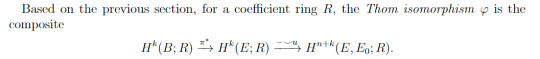
Thom Isomorphism & the Euler Class

As promised, another longpost. This one might be a bit more technical than others I've done recently, but hopefully still approachable to someone who's done a reasonable course in algebraic topology (Ch 1-3 of Hatcher) and also knows what a fibre/vector bundle is. The end goal will be to introduce the Euler class as a generalisation of the Euler characteristic, and to motivate characteristic classes more generally.

A Brief Note on Vector Bundles

It's always difficult to know where to start with these things, but let's assume that you know what a vector bundle is, and that I don't have to motivate working with them. In case you've only seen them for manifolds before, observe that the definition works just as well for any reasonably nice space - I'll assume everything is a CW complex, although CW approximation means I don't actually have to.

A more interesting idea is this. To any manifold M, we have a canonical vector bundle TM, the tangent bundle. So if something is a property of manifolds, we can ask whether it is actually a property of TM, and if so, can it be generalised to other vector bundles? Suprisingly the answer is often yes.

The Leray-Hirsch Theorem

I can't prove everything, so let's state a theorem that we'll use later. Ignore the theorem numbering, and cohomology is taken with R-coefficients.

You should think of this as a version of the Kunneth theorem, that generalises from products to more general fibre bundles. Condition (i) is just a rephrasing of the vanishing of the Tor term - like the in the Kunneth theorem, it's automatic if we take R to be a field. (ii) is a niceness condition on the bundle, and it's a good exercise to check that it will be satisfied for a product.

I actually lied slightly, we're going to use a relative version of this. But like always in algtop, if you can believe the absolute version, you can believe the relative version.

The Thom Space

Suppose we have a rank n vector bundle π: E -> B. This is a bit annoying algebraically, because E homotopy retracts onto B no matter how twisted it is. So to capture any non-triviality we need to be a little bit clever. First, observe that we get a disc bundle π: D(E) -> B by just choosing a closed disc in fibre. (If we're in a manifold, choose a metric and take the unit disc. If we're not, you have to work a little harder to show this is well-defined). Now D(E) is a manifold with boundary, which is a sphere bundle S(E) -> B. Take the quotient D(E)/S(E) by collapsing the whole boundary to a point. We call this the Thom space T(E) of the vector bundle. Notice that T(E) is uniquely determined by π, but is definitely non-trivial!

As an example, take B= S^1, and consider the two line bundles. If E is the orientable line bundle, T(E) looks like a sphere with two points identified, so is homotopy equivalent to S^1 v S^2 [exercise]. If E is the non-orientable line bundle, then T(E) is RP^2.

You might notice that this is no longer a fibre bundle over B, as the point S(E)/S(E) lives in every "fibre". Oh well. It does have a nice CW decomposition though! First , give T(E) a single 0-cell, the point S(E)/S(E). Then suppose B has a fine enough decomposition that π is trivial over each cell [this is actually automatic, bc discs are contractible]. Each i-cell in B lifts to a (i+n)-disc in D(E), and under the quotient this is an (i+n)-cell in T(E). Like in my last post, you have to do a little bit of work to check that this really is a CW decomposition, but hopefully you believe me. You should double check with the line bundles over a circle that these do in fact give the usual cell structures.

Now, let's make the reasonable assumption that B is connected with a single 0-cell, so T(E) has one 0-cell, one n-cell, and no cells of dimension 1,...,n-1. Let's also suppose that π is R-oriented; that is, either the vector bundle is oriented and R is any ring, or it is unoriented and R = Z/2. Then the coboundary map of the n-cell to he (n+1)-cells is trivial [exercise: think about the boundary map from the 1-cells to the 0-cell in B]. In particular, H^n(T(E)) = R, and has a canonical generator coming from the choice of orientation! We call this the Thom class of E.

The Thom Isomorphism

More often, we work in relative cohomology, using the fact that

H^*(T(E)) = H^*(D(E), S(E)) = H^*(E,E\B).

Here the first isomorphism is the usual relative <--> quotient; the second is excision, and I'm identifying B with the 0-section. This is nice for the following reason. Given a choice of orientation, on each fibre F of E, we have a canonical generator of H^n(F, F\0). [This is possibly your definition of orientation, but if not then it's equivalent]. The Thom class is a class in H^n(E,E\B) that restricts to the generator on the fibre over the 0-cell. But the 0-cell was chosen arbitrarily, so in fact it restricts to the generator on every fibre! It's not obvious that such a class exists, so it's nice to see that it does.

Finally, let's apply the (relative) Leray-Hirsch theorem. H^i(F,F\0) is free for all i since F is just a vector space; condition (ii) is met by the Thom class! We can then make two final simplifications. Firstly, H^*(B) is isomorphic to H^*(E) by pulling back under π. Secondly, H^i(F,F\0) is either 0 or R, so vanishes in the tensor product. Putting it all together, we get the following.

Phew! That's a lot of work, and we haven't even gotten to the Euler class yet.

The Euler Class

This is surprisingly easy. Remember that the Thom class lives in relative cohomology H^n(E,E\B). We can always pull back a relative class under inclusion to an absolute class u' ∈ H^n(E). Identifying this with H^n(B) again by π, we get the Euler class e(π) ∈ H^n(B)

Sometimes it's more helpful to think of it as follows. By the abstract nonsense that is the relative cup product, u⌣u = u'⌣u. So we get the following equivalent definition:

This can be nicer to work with, as u⌣u is a square so has some nice properties. For example, take the following basic facts:

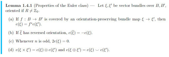
(a) is true by checking that the Thom class pulls back - this follows directly from viewing it as the unique class restricting to the generator on fibres.

(b) is true by the same observation.

(c) is quite hard to prove using the first definition that we gave, but it follows directly from the fact that u⌣u = -u⌣u if n is odd. Note that this is a weaker version of the statement that the Euler characteristic of an odd dimensional manifold is 0!

(d) These are both actually kinda tricky, but it's not hard to convince yourself it's true.

Ok this post is already way too long, so I'll delay the main point until next time, when I'll link the Euler class to Poincare duality, and eventually to the actual Euler characteristic. For now, a teaser of why else it might be useful:

The first bullet follows directly from (c)+(d) above. For the second, suppose we had a nowhere-zero section s: B -> E\B. Writing i for the inclusion E\B -> E, we get the composite πis = id_B. But π^*e(π) = u' by definition, and i^* u' = 0 since u' is the pullback of a relative class! So e(π) = s^*(0) = 0.

As a sanity check for where we're going, recall that S^1 and S^3 have nowhere-zero vector fields while S^2 doesn't. The Euler characteristic of S^1 and S^3 is zero, while the Euler characteristic of S^2 is 2. This is looking promising!

[michaelrotonal]

cool math thing i'm wondering about

are there infinitely many primes of the form n^2+1?

you'd think you could figure it out easily but no

list of thoughts on this:

numbers of the form n^2+1 cannot be divisible by numbers that are 3 mod 4.

each prime of the form 1 mod 4 only has 2 values of n where n^2+1 is divisible by it

this is isomorphic to "are there infinitely many gaussian primes of the form n+i?"

each individual prime factor only blocks out at most half of the n values, but every n value hits some prime factor. i feel like there's no way that at some point every n value hits two prime factors.

there are two ways to prove that for any prime, there's a n^2+1 that doesn't include any primes up to it.

way one is by picking an appropriate remainder for each prime, and using the chinese remainder theorem to find an n that works

the other way is just multiplying all the primes up to it and taking that as your n

if you're reading this, i'd like to invite you to reblog with any of your own thoughts you may have on this problem that are not already there

every prime that is 4n+1 can be written as a sum of two squares, but the question is how often is one of those squares 1?

sums of two squares are nice because you can multiply together two of them and make another new one of them

how is this conjecture not on wikipedia yet though. it seems like such a simple thing to ask

[lipshits-continuous]

Explanation Posts

I explain my url (continuity in ℝ) 05/06/2022

Definition of a Ring 07/10/2022

Definition of a Metric Space 16/10/2022

Open and Closes sets in a Metric Space 16/10/2022

Convergence and Continuity in Metric Spaces 22/10/2022

Bounded and Compact sets in a Metric Space 23/10/2022

I show 0.9999...=1 30/11/2022

Linear Maps and Isomorphisms 18/01/2023

Ring homomorphisms, Ideals, Quotients, and the First Isomorphism Theorem 12/03/2023

Mutamorphic Functions (technically not an explanation post but still belongs here) 29/06/2023

Second Countability of ℝⁿ 04/07/2023

The Weierstrass Function 23/08/2023

Unbroken Workbrooks (A post about continuity written in Anglish) 19/09/2023

Countable Sets have 0 Lebesgue Outer Measure 17/10/2023

Introduction to Homotopy 05/02/2024

The Fundamental Group 16/02/2024

Continuity in Terms of Open Sets 16/02/2024

The Set of Finitely Generated Free Groups as a Monoid 01/03/2024

Intro to Topology: Metric Spaces 12/03/2024

Intro to Topology: Topological Spaces and Continuity 19/03/2024

Intro to Topology: Closed Sets and Limit Points 26/03/2024

Intro to Topology: Hausdorffness 26/03/2024

Intro to Topology: Connectedness 27/03/2024

Intro to Topology: Path Connectedness 28/03/2024

Intro to Topology: Compactness 11/04/2024

Intro to Topology: Bases and Second Countability 12/04/2024

Intro to Topology: Product Spaces 23/04/2024

Intro to Topology: The Heine-Borel Theorem 24/04/2024

Intro to Topology: Quotient Spaces 25/04/2024

Intro to Topology: Important Examples 26/04/2024

Intro to Topology: Conclusions and Remaining Questions 26/04/2024

The Dirac Delta Distribution is not an Extended Real Function 03/05/2024

The Fundamental Group of a Topological Group is Abelian 10/06/2024

Proof of the Factor Theorem 30/06/2024

A Short Intro to Category Theory 23/10/2024

An Example of When Connectedness Implies Path Connectedness 17/11/2024

Relative de Rham Cohomology 13/06/2025

[mantacid]

I would go absolutely feral if there turned out to be a mathematical object isomorphic to a proof. The amount of chaos I could cause would be legendary.

"Assume there exists a set S_A, defined as the set of pairs (h,p) -- where h is an element of the set of theorems, and p is an element of the set of proofs -- under a set of axioms A.

Define T_A to be the subset of S_A where each element satisfies the following: (h,p) is in T_A if and only if p either proves or disproves h.

For convenience, let us define a set R_A containing pairs (h,b) where h is once again in the set of theorems, and where b is a Boolean. We can say that a proof is similar to a morphism p:H -> Bool; in other words, a proof turns a hypothesis into a statement of truth or falsehood. If such a morphism does not exist for a theorem in the domain, then we can conclude that the axioms of set A do not allow for a conclusive answer (see: Gödel's theory of incompleteness).

Now, consider the subset of T_A containing all currently unsolved millennium prize problems..."