#path matrix representation of graph

[jeremy-ken-anderson]

An adjacency list in a graph is a series of numbers that tells you how many nodes are adjacent to each node. So if you imagine a 3x3 square of rooms that all connect with a door in the center of each wall, the corner rooms would have a value of 2 (the side rooms adjacent to them), the side rooms would have a value of 3 (the adjacent corner rooms and the center), and the center would have a value of 4 (being adjacent to all 4 side rooms).

An adjacency matrix for a graph is possibly more confusing, depending on how your brain works, but defaults to containing more info and has faster lookups in terms of computer processing. It would represent those 9 rooms as a 9x9 grid and mark each door you could go out of as a 1 instead of a 0. So

becomes

And you can see it's symmetrical (split down the line of Xs), because you can go through a door either direction. If these were streets in a city and the street going from intersection E to F was a one-way street, the E,F would be a 1 but the F,E would be a 0.

To get a 2-hop option - everything available in 2 jumps from each point, allowing for overlap - you do slightly different things depending on whether List or Matrix is your representation.

For a List, you have a nested for loop, grabbing the set of adjacent options in the outer loop, and asking for them to spit out a list of their adjacent options in the inner loop. Imagine a 4-square of rooms

J Q K A

the outer loop would say, What's adjacent to J? Q- What's adjacent to Q? J and A are adjacent to Q K- What's adjacent to K? J and A are adjacent to K What's adjacent to Q? J- What's adjacent to J? Q and K are adjacent to J A- What's adjacent to A? Q and K are adjacent to A and so on. So the 2-hop for J ends up with J,A,J,A, for Q it's Q,K,Q,K, for K it's Q,K,Q,K, and for A it's J,A,J,A.

For matrices you do Matrix Multiplication. For square matrices of the same size (which works perfectly for us because we're trying to square the matrix in the first place) you take the row and column that meet at each point in the matrix and multiply across. If you were squaring a matrix

your new A would be A*A + B*D + C*G. Your new B would be A*B + B*E + C*H.

So the square of

For A,A it's a,a(0)*a,a(0) + b,a(1)*a,b(1) ... + i,a(0)*a,i(0) = 2 For B,A it's a,a(0)*b,a(1) + b,a(1)*b,b(1) ... + i,b(0)*b,i(0) = 0

And this makes sense. Remember, this is representing how many paths there are to go from one space to another in exactly 2 jumps. A,A means "how many paths go from A back to A in 2 steps." You can see there are 2: A -> B -> A and A -> D -> A. There's no way to actually take 2 steps starting from B and get to A. Using this logic we can guess by looking at the "map" that B,H would give us a value of 1, because there's only one way to get from B to H in 2 hops.

If we do the same cross-section trick to multiply it out, we have 1*0 + 0*0 + 1*0 + 0*0 + 1*1 + 0*0 + 0*1 + 0*0 + 0*1 and sure enough, we have just one spot where the numbers match up.

[programmingandengineering]

CS590 homework 6 – Graphs, and Shortest Paths

Develop a data structure for directed, weighted graphs G = (V, E) using an adja­cency matrix representation.. The d.atatype int is used to store the weight of edges. int does not allow one to represent ±co. Use the values INTYIN and IN’T_MAX (defined in limits .h) instead. include <limits-h5 in.t d, e; d = INT_MAX; e = INT_MIN; if (e == ih–r_mir;) if (d I = IN–1_102A10           . Develop a…

[emilyratajkowski164395]

In network science, embedding refers to the process of transforming nodes, edges, or entire network structures into a lower-dimensional space while preserving the network's essential relationships and properties. Network embeddings are particularly valuable for machine learning applications, as they allow complex, non-Euclidean data (like a social network) to be represented in a structured, high-dimensional vector format that algorithms can process.

Building on the concept of embeddings in network science, these transformations unlock several advanced applications by enabling traditional machine learning and deep learning methods to operate effectively on graph data. A key advantage of embeddings is their ability to encode structural and relational information about nodes in a network into compact, dense vectors. This allows complex, sparse graphs to be represented in a way that preserves both local connections (like close friendships) and global structure (like communities within the network).

There are multiple approaches to generating these embeddings, each with its own strengths:

Random Walk-based Methods: Techniques like DeepWalk and node2vec use random walks to capture the network’s context for each node, similar to how word embeddings like Word2Vec capture word context. By simulating paths along the graph, these methods learn node representations that reflect both immediate neighbors and broader network structure.

Graph Neural Networks (GNNs): Graph neural networks, including variants like Graph Convolutional Networks (GCNs) and Graph Attention Networks (GATs), use neural architectures designed specifically for graph data. GNNs aggregate information from neighboring nodes, creating embeddings that adaptively capture the influence of each node’s surroundings. This is especially useful in tasks that require understanding both individual and community-level behavior, such as fraud detection or personalized recommendations.

Matrix Factorization Techniques: These methods, like LINE (Large-scale Information Network Embedding), decompose the graph adjacency matrix to find latent factors that explain connections within the network. Matrix factorization can be effective for representing highly interconnected networks, such as knowledge graphs, where the relationships between entities are intricate and abundant.

Higher-order Proximity Preserving Methods: Techniques like HOPE (High-Order Proximity preserved Embeddings) go beyond immediate neighbors, capturing higher-order structural relationships in the network. This approach helps model long-distance relationships, like discovering latent social or biological connections.

Temporal Network Embeddings: When networks evolve over time (e.g., dynamic social interactions or real-time communication networks), temporal embeddings capture changes by learning patterns across network snapshots, allowing predictive tasks on network evolution, like forecasting emerging connections or trends.

Network embeddings are powerful across disciplines. In financial networks, embeddings can model transaction patterns to detect anomalies indicative of fraud. In transportation networks, embeddings facilitate route optimization and traffic prediction. In academic and citation networks, embeddings reveal hidden relationships between research topics, leading to novel insights. Moreover, with visualization tools, embeddings make it possible to explore vast networks, highlighting community structures, influential nodes, and paths of information flow, ultimately transforming how we analyze complex interconnections across fields.

[myprogrammingsolver]

CS590 homework 6 – Graphs, and Shortest Paths

Develop a data structure for directed, weighted graphs G = (V, E) using an adja­cency matrix representation.. The d.atatype int is used to store the weight of edges. int does not allow one to represent ±co. Use the values INTYIN and IN’T_MAX (defined in limits .h) instead. include <limits-h5 in.t d, e; d = INT_MAX; e = INT_MIN; if (e == ih–r_mir;) if (d I = IN–1_102A10           . Develop a…

[lupinepublishers]

Lupine publishers|The Spectral Characterization of Hamiltonicity of Graphs

The Spectral Characterization of Hamiltonicity of Graphs

Introduction It is an important NP-complete problem in structure graph theory to judge whether a graph is Hamiltonian. So far, there is no perfect description on this problem. Therefore, it has always been concerned by the workers of graph theory and mathematics. It is explored that the new method for characterization of Hamiltonicity of graphs. Because the spectrum of a graph can well reflect the structural properties of a graph and is easy to calculate, at the 2010 conference of the theory of graph spectra, M. Fiedler and V. Nikiforov formally proposed whether the theory of graph spectra can be used to study the Hamiltonicity of a graph, and they [1] gave sufficient conditions for given graph to be Hamiltonian (or traceable) in terms of the spectral radius of the graph. Since then, relying on the spectrum of matrix representation of graph, giving the spectral sufficient conditions of the Hamiltonian graph has been a new method to study the Hamilton problem. Many results have been obtained by using the spectral radius and the signless Laplacian spectral radius of the graph to describe the Hamiltonicity of the graph. [2] firstly gave a sufficient condition for a graph G to be Hamiltonian and traceable by using the signless Laplacian spectral radius of the complement of the graph [3] optimized the condition of the number of edges of the Hamilton graph, gave a better condition for G to be traceable by using the spectral radius of the graph G, and firstly gave a sufficient condition for the balanced bipartite graph to contain the Hamilton cycle by the spectral radius of its quasi-complement graph. [4] firstly used the spectral radius and signless Laplacian spectral radius of the graph to describe the Hamilton-connected of the graph. [5] used the signless Laplacian spectral radius of the quasi-complement graph of the balanced bipartite graph to give a sufficient condition for the balanced bipartite graph to be Hamiltonian and used the signless Laplacian spectral radius of the graph G to give a sufficient condition for the graph G to be traceable or Hamilton-connected. [6] continued to study the relationship between the Hamiltonicity and spectral radius of general graphs and balanced bipartite graphs and extended the conclusions in [3] and [5]. [7] firstly proposed to use the stability of graphs to study the Hamiltonian properties of graphs, and also summarized the method of studying the spectral characterization of the Hamiltonian graph by optimizing the boundary conditions of the Hamiltonian graph. [8] firstly characterized traceability of connected claw-free graphs by spectral radius. [9] discussed spectral conditions for Hamiltonicity of claw- free graphs. [10] firstly presented spectral sufficient conditions for a k-connected graph to be traceable or Hamilton-connected. [11] firstly presented sufficient conditions based on spectral radius for a graph to be k-connected, k-edge- connected, k-Hamiltonian, k-edge-Hamiltonian, β-deficient and k-path-coverable. Lately, [12] firstly gave spectral radius or signless Laplacian spectral radius conditions for a graph to be pancyclic. Because the minimum degree of a graph is related to the density of the graph, with the deepening of research, people began to study the spectral characterization of Hamiltonian properties of graphs with large minimum degree conditions and gave the better conclusions. By adding the condition of large minimum degree, [13] firstly presented some (signless Laplacian) spectral radius conditions for a simple graph and a balanced bipartite graph to be traceable and Hamiltonian, respectively. Subsequently, [14] optimized the lower bound of the spectral condition of simple graphs with large minimum degree; [15]

optimized the lower bound of the spectral condition of balanced bipartite graphs with large minimum degree. [16] characterized the signless Laplacian spectral radius conditions for a graph or balanced bipartite graph with large minimum degree to be Hamiltonian. [17] and [18] studied the signless Laplacian spectral radius condition for a graph with large minimum degree to be Hamilton-connected. [19] presented some spectral radius conditions for a balanced bipartite graph or a nearly balanced bipartite graph with large minimum degree to be traceable, respectively. [20] gave some spectral sufficient conditions for a balanced bipartite graph with large minimum degree to be traceable and Hamiltonian in terms of the spectral radius of the graph with large minimum degree. It strengthened the according results of Li and Ning for n sufficiently large. [21] presented some conditions for a simple graph with large minimum degree to be Hamilton-connected and traceable from every vertex in terms of the spectral radius of the graph or its complement respectively

and gave better conditions for a nearly balanced bipartite graph with large minimum degree to be traceable in terms of spectral radius, signless Laplacian spectral radius of the graph or its quasi-complement respectively. [22] presented sufficient spectral conditions of a connected graph with large minimum degree to be k-hamiltonian or k-path-coverable or β-deficient, for relatively large n. [23] gave the sufficient conditions for a graph with large minimum degree to be s-connected, s-edge-connected, β-deficient, s-path-coverable, s-Hamiltonian and s-edge-Hamiltonian in terms of spectral radius of its complement. Other spectral characterizations on Hamiltonicity, at present, only [24,25] used the Laplacian eigenvalues to give the spectral sufficient condition for the graph to be Hamiltonian. [26] firstly applied the distance signless Laplacian spectral radius of the graph’s complement to give a sufficient condition for the graph to be traceable or Hamiltonian. [27] firstly discussed the Hamiltonian in terms of the energy of graph. [28], by adding the maximum degree condition on the basis of [26], used the energy of complement graph to give the sufficient conditions for the graph to be traceable, Hamiltonian and Hamilton-connected. The results optimized the conclusions of [26] in a sense. [22] gave some sufficient conditions for a nearly balanced bipartite graph with large minimum degree to be traceable in terms of the energy, the first Zagreb index and the second Zagreb index of the quasi-complement of the graph, respectively. By observing, we find that the conditions of all the above conclusions deduce that the graphs are dense. In fact, there are many Hamiltonian graphs with non dense edge distribution, such as cycles. Therefore, it is necessary to study whether a non- dense graph (sparse graph) is a Hamiltonian graph, but there are few research results. Komlos and Szemeredi proposed that almost all graphs are Hamiltonian graphs in 1975. Inspired by this, [29] characterized the Hamiltonian property of regular graphs by using the adjacency spectrum of graphs; [30] characterized the Hamiltonian property of almost regular graphs by using the Laplace spectrum of graphs. In 2011, Radcliffe proposed whether we can give sufficient conditions for Hamiltonian graphs by using the normal Laplace spectrum of graphs. In 2012, [31] studied this problem, gave corresponding conclusions, and explained that the conclusions are applicable to the determination of Hamiltonicity of general graphs. Although there are a lot of results, there are still many problems worthy of further study. Firstly, combining the ideas from theorems of Ore and Fan to develop extremal spectral conditions for dense graphs (with given connectivity, toughness, forbidden subgraphs) to be Hamiltonian (or related structural properties). Such as, finding spectral sufficient conditions for a graph or its complement to be Hamilton-connected, or k-Hamiltonian, k-path-coverable, k-edge-Hamiltonian; signless Laplacian spectral radius sufficient conditions for a (nearly) balanced bipartite graph or its nearly complement to be traceable, or Hamiltonian; (signless Laplacian) spectral radius sufficient conditions for the nearly complement of a balanced bipartite graph to be bipancyclic or considering the case with minimum degree; the characterization of Hamiltonicity of graphs with 1-tough [32,33]. Secondly, due to the difficulty of research, there are only three papers to study Hamiltonian properties of sparse graphs, but there are many sparse Hamiltonian graphs. Therefore, there is a lot of space to explore some sufficient or necessary conditions for sparse graphs with some properties to be Hamiltonian (or related structural properties) by using the spectrum of the graph and corresponding

eigenvector. At last, directed graphs also have Hamiltonian properties, but all previous studies have only considered undirected graph. So, it is also very valuable to study extremal spectral conditions for oriented graphs to be Hamiltonian. The research on the spectral characterization of Hamiltonicity of graphs build a bridge between structure graph theory and algebraic graph theory. Expected results not only enrich the study of Hamilton problem in structural graph theory, but also extend the spectral study of algebraic graph theory, thus promoting the research of algebraic method of Hamilton problem. Acknowledgements Supported by the Natural Science Foundation of China (No. 11871077), the NSF of Anhui Province (No. 1808085MA04), the NSF of Department of Education of Anhui Province (No. KJ2020A0894), and Research and innovation team of Hefei Preschool Education College (No. KCTD202001).

For more information about Journal of Anthropological and Archaeological Sciences archive page click on below link

https://lupinepublishers.com/anthropological-and-archaeological-sciences/archive.php

For more information about lupine publishers page click on below link

https://lupinepublishers.com/index.php

[codezclub]

C Program to find Path Matrix by powers of Adjacency matrix

Path Matrix by powers of Adjacency Matrix Write a C Program to find Path Matrix by powers of Adjacency Matrix. Here’s simple Program to find Path Matrix by powers of Adjacency Matrix in C Programming Language. Adjacency Matrix:  Adjacency Matrix is a 2D array of size V x V where V is the number of vertices in a graph. Let the 2D array be adj[][], a slot adj[i][j] = 1 indicates that there is an…

[manikarea]

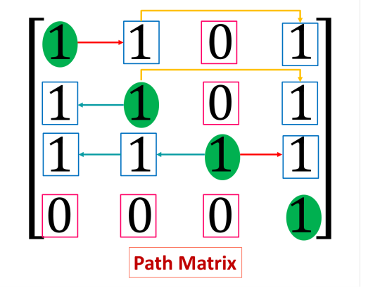
Path Matrix in Data Structure with Example

Path Matrix in Data Structure with Example

Path Matrix refers to a special type of data representation in data structure specially in graph theory. Path Matrix represents the availability of a path from a node to another node. What is Path Matrix? A path matrix is a matrix representing a graph, where each value in m’th row and n’th column project whether there is a path from node m to node n. The path may be direct or indirect. It may…

[highgradewriters22]

What in your opinion is the single most important motivation for the development of hashing schemes while there already are other techniques that can be used to realize the same functionality provided by hashing  methods? 

Given a directed graph, described with the set of vertices and the set of edges,  · Draw the picture of the graph· Give an example of a path, a simple path, a cycle· Determine whether the graph is connected or disconnected· Give the matrix representation of the graph· Give the adjacency lists representation of the graphEssay Question: What in your opinion is the single most important motivation…

[kitwallace]

Finding Eulerian circuits

As discussed previously, Eulerian circuits are useful in 3D printing because they enable continuous extrusion which increases the strength of the printed object . In addition the lack of a seam improves its visual appearance.  

However finding a Eulerian circuit in a design is not always easy, and finding the ‘best’ even harder.

For a rectangular grid  (3 x 2) 

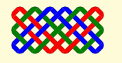
a braiding program I developed a while ago finds a circuit.  It attempts to find a braid on an N x M grid.  If N and M are relatively prime, one rope (ie. a Eulerian circuit) completes the grid  but if not (like this 6 x 3), multiple ropes are needed.

This restriction on the size of this mesh is not helpful.  Since every N x M mesh of this style is Eulerian, they must all have a Eulerian circuit. This could  be constructed if we were able to join up the separate partial loops. Start somewhere and follow a chain of unvisited edges until you get back to the start.  If all edges have been visited, you are done. If not, go back to the last vertex with unvisited edges and start a new circuit at that point, with those points inserted into the current circuit .This is the Hierholzer algorithm.

Hierholzer algorithm

I searched for a pseudo code implementation but wasn’t satisfied with any that I found.  Any implementation depends heavily on the data structures used: for the graph itself in a form in which edges can be removed as they are visited and for the path as it is constructed, adding a vertex to the end and rotating the path to backtrack. 

One representation of a graph with V vertices and E edges is as a V x V adjacency matrix where adj[i,j] =1 indicates the edge i to j which will be symmetric across the diagonal if the graph (as here) is undirected.  Updating is straightforward but  navigating from vertex to vertex requires a scan through a row.  

Alternatively, the graph can be represented as an array of lists of the connected vertices  - easy to navigate, more compact for a sparse graph (as these are)  but harder to update.  

The JavaScript array structure can implement the vertex list and the evolving path. I found this is a useful summary of operators. push() and pop()  will add and remove the head of the list;  unshift() and shift() do the same at the tail of the list.  myArray[myArray.length - 1] and myArray[0] return the head and tail of the list respectively.

Minimizing turns in the circuit

The Hierholzer algorithm mechanically selects the next vertex by taking any vertex (the first or the last perhaps) from the list of possible vertices. This does find a circuit but not necessarily a good circuit.  For the purposes of 3D printing, good means a circuit with a minimum number of turns since straight runs will be stronger and faster.  To get a good, though not necessarily the best, circuit, I added a kind code to each edge and then choose a vertex in the same kind if possible.  For the rectangular mesh above, there are two kinds , coded +1 for the right diagonal, -1 for the left.  (note that we don’t need to distinguish between the direction of travel on a diagonal since we can’t reverse direction at a vertex as that edge has just been traversed)

JavaScript Implementation

In the Fottery suite, the algorithm is implemented as a method in a Graph class which includes the adjacency structure adj and supporting functions:

find_circuit(kind-0,start_vertex = 0 ) {    // assumes graph is connected and a euler circuit exists         var cpath =[];        var vertex, next_vertex, edge, edges;        cpath.push(start_vertex);        while (cpath.length < this.n_edges  ) {            vertex = cpath[cpath.length - 1];  // the last vertex in the constructed path            edges = this.adj[vertex];  // get its  adjacent nodes (untraversed edges)            if (edges.length == 0) {  // if no untraversed edges                cpath.pop();   // rotate back to the previous vertex                if (!(vertex == initial_vertex && cpath[0]==vertex)) { // dont  include the start at the end                  cpath.unshift(vertex);                 }            } else {                  edge = this.best_edge(edges,kind);                  next_vertex= edge[0];                kind = edge[1];                cpath.push(next_vertex);  // add  vertex to the path                this.remove_edge(vertex,next_vertex); // remove the traversed edge            }         }

       // get start back to the first in the path        while (cpath[0] != start_vertex)                  cpath.push(cpath.shift());        return cpath;

[damn discovered a use-case where this implementation fails!   

16 April 2024 - fixed edge case with the bold change ] 

Example

A  rectangular N x M  mesh like the one above is more useful if the vertices at the edges are connected to make a border.  This addition does not change the Eulerian nature of the graph, but introduces two more directions, horizonal and vertical.  This is the resultant 2 x 3 mesh.

and this a box constructed from rectangular meshes.  The sides are bevelled by insetting the top layer from the bottom by the thickness of the tile to make a 45 degree bevel.  Assembled with plastic glue (UHU).

Stars (stellated polygons)

This algorithm has been applied to other structures such as a triangular mesh and stars.   

A pentagram can be constructed with 5 vertices and 5 edges connecting pairs of vertices.This is a closed path so Eulerian.

A hexagram looks Eulerian, but if constructed by connecting the vertices of the star, the graph is not connected (two separate triangular paths).

To make a circuit so it can be printed continuously, we have to compute the 6 intersections and the 18 edges (of 3 kinds)  which result from the intersections, and then use the modified Hierholzer algorithm to find a good circuit.  

A fully connected star is only Eulerian if the number of vertices is odd - which makes for a kind of infill pattern.

Nearly Eulerian graphs

Structures which are Eulerian are rather limited. An hexagonal tiling is not Eulerian because vertices are order 3. However it and many others are nearly Eulerian in the sense that small modifications to the graph will make the graph Eulerian. The basic idea is to duplicate ( the minimum number of ) edges. If this is a problem with printing, the edge could be omitted or an additional edge inserted.

This problem  is called the Chinese Postman Problem or Route Inspection Problem and the subject of extensive research. 

This is work for another day -.April 2024 see Non-Eulerian graphs

References

Fleischner, Herbert (1991), "X.1 Algorithms for Eulerian Trails”   https://archive.org/details/euleriangraphsre0001flei/page/

Gregory Dreifus,Kyle Goodrick,Scott Giles,Milan Patel Path Optimization Along Lattices in Additive Manufacturing Using the Chinese Postman Problem June 2017  https://www.researchgate.net/publication/317701126_Path_Optimization_Along_Lattices_in_Additive_Manufacturing_Using_the_Chinese_Postman_Problem

Prashant Gupta, Bala Krishnamoorthy, Gregory Dreifus  Continuous Toolpath Planning in a Graphical Framework for Sparse Infill Additive Manufacturing  April 2021 https://arxiv.org/pdf/1908.07452.pdf

https://algorithms.discrete.ma.tum.de/graph-algorithms/directed-chinese-postman/index_en.html

https://www.stem.org.uk/resources/elibrary/resource/31128/chinese-postman-problems

https://ibmathsresources.com/2014/11/28/the-chinese-postman-problem/

http://www.suffolkmaths.co.uk/pages/Maths%20Projects/Projects/Topology%20and%20Graph%20Theory/Chinese%20Postman%20Problem.pdf

[jeremy-ken-anderson]

A matrix representation of a graph of a square with doors going from 1-2 and back, 2-3 and back, 3-4 and back, and 4-1 and back, would look like this 0101 1010 0101 1010 Each node has a total degree of 4. In spite of using a door as an analogy the "degree" counts the fact that there's a path out to and in from those adjacent rooms. Looking at the matrix you can get the same result by adding up the number of 1s in the matching row and column. In row 3 there are two 1s, indicating the means to go out to rooms 2 and 4. In column 3 there are two 1s, indicating the ability to come in from rooms 2 and 4.

Now imagine the same square but it's all 1-way streets. You can only go from 1-2, from 2-3, from 3-4, and from 4-1. It looks like so: 0100 0010 0001 1000 You can see that the matrix still shows the correct information. Row 1 column 2 has a 1 in it, so you can go from 1 to 2. Row 4 column 1 has a 1 in it, so you can go from 4 to 1. And between row 1 and column 1 you have a total of two 1s, so the first node has a degree of two.

The adjacency list representation of the "doorways" is like this:

1 - (2,4) 2 - (1,3) 3 - (2,4) 4 - (1,3)

The list representation is nice when you've got big areas described, because you may have noticed that even with just a square there's a lot of needless 0s telling you "there's not a line between these two points going this direction." With the list you only bother to say something exists when it's something existing.

[thousandmaths]

Coxeter Transformations

This talk was given at the student combinatorics seminar by Emine Yildirim, as a pre-talk for the talk she would give the next day at the adult seminar. So there wasn’t too much in this talk about Coxeter Transformations; the majority of the talk was in fact about path algebra representations.

This post is not totally elementary but should be accessible if you have some algebraic background; for instance, if you’ve read the associative algebras sequence.

------

Bound Quiver Algebras

Rather than studying path algebras $kQ$ per se, we want to study a particular selection of their quotients.

Definition. Let $R_Q$ be the two-sided ideal generated by arrows. An ideal $I\subseteq kQ$ is called admissible if there exists some $m$ such that $R_Q^m \subseteq I \subseteq R_Q^2$.

This definition is a little opaque, but it actually has a very simple combinatorial description: an admissible ideal is supposed to contain all sufficiently long paths, and is supposed to not contain ��paths” that only use a single edge.

The purpose of an ideal is to take a quotient. The fact that admissible ideals contain all long paths means that the quotient $kQ/I$ will be finite-dimensional, which makes it more amenable to understanding combinatorially. We say that this quotient $kQ/I$ is the bound quiver algebra associated to $I$.

Considering the rather concrete setup of this situation, the following theorem may surprise you:

Theorem. Suppose that $A$ is a connected finite-dimensional algebra whose simple modules are all one-dimensional. Then there exists a directed graph $Q$ and an admissible ideal $I$ such that $A\cong kQ/I$.

[ The property of having all simple modules be one-dimensional is called “basic”. I’m glad she mentioned this because, as you imagine, googling “basic algebra” does not yield the most helpful results. ]

------

Our Favorite Modules 

In a talk I wrote up previously, we saw an explicit construction of the indecomposable simple and projective modules of a path algebra:

$S_v$ consists of all multiples of $e_v$, the do-nothing path starting at $v$.

$P_v$ is spanned by all paths starting at $v$.

There is also one more important type of indecomposable module called an injective module. In general, injective and projective modules are “dual” in a technical sense; we see the duality in this concrete setting quite clearly:

$I_v$ is spanned by all paths ending at $v$.

These definitions behave well with respect to quotients, and in particular the definitions are word-for-word identical in bound quiver algebras. (Of course, word-for-word identical doesn’t mean that the objects are the same, since, for instance, many of the paths starting at $v$ will be sent to zero in the quotient.)

The utility of the injective modules are a lot harder to describe than that of the projectives (and it’s already not so easy to describe the utility of the projectives). Let me wave my hands in air, shout “Auslander-Reiten”, and try to be satisfied.

------

Our (new) Favorite Matrix

Associated to any directed graph is a matrix called its Cartan matrix $C$, whose entries $c_{ij}$ are defined as the number of paths from $j$ to $i$. From this definition one sees that the sum of all the entries in the $j^\text{th}$ column is the dimension of $P_j$ and the sum of all the entries in the $i^\text{th}$ row is the dimension of $I_i$. 

In fact, one can obtain considerably more information from the Cartan matrix than this if one knows about quiver representations. Just as in the unbound case, the bound case also has an equivalence of categories $\textbf{Mod}(kQ/I)=\textbf{Rep}(Q; I)$; the latter notation means that the maps corresponding to paths in $I$ vanish. Then: the columns and rows of the Cartan matrix are precisely the dimension vectors of $P_j$ and $I_i$ as quiver representations.

From the Cartan matrix, one can easily construct something called the Coxeter transformation: it is $-C^TC^{-1}$. The significance of the Coxeter transformation is that it “takes projectives to injectives” in the following sense: if you apply the Coxeter transformation to the dimension vector of $P_v$, the output is the dimension vector of $I_v$.

There is, of course, no great reason to expect any nice linear-algebraic properties of the Coxeter transformation. But miraculously, it seems to be surprisingly well-behaved. In particular, in many cases the Coxeter transformation has finite order (that is, if you do the Coxeter transformation, and then do it again, and then do it again, and then... then eventually you get back to the same vector you started with). 

[ In the Q&A, someone asked if there was any combinatorial meaning to be given to the other elements in the orbit of $P_v$. Yildirim didn’t know, but she seemed to find the question interesting. ]

This certainly doesn’t hold for every quiver, but it seems to be true in particular for quivers associated to Coxeter groups. For instance, if $Q$ is an oriented Dynkin diagram, then the Coxeter transformation has finite order, and in fact the order is precisely the Coxeter number $h$ (i.e. the order of any Coxeter element).

[ Post 1 ] [ Next ]

[sciforce]

Towards Automatic Text Summarization: Extractive Methods

For those who had academic writing, summarization — the task of producing a concise and fluent summary while preserving key information content and overall meaning — was if not a nightmare, then a constant challenge close to guesswork to detect what the professor would find important. Though the basic idea looks simple: find the gist, cut off all opinions and detail, and write a couple of perfect sentences, the task inevitably ended up in toil and turmoil.

On the other hand, in real life we are perfect summarizers: we can describe the whole War and Peace in one word, be it “masterpiece” or “rubbish”. We can read tons of news about state-of-the-art technologies and sum them up in “Musk sent Tesla to the Moon”.

We would expect that the computer could be even better. Where humans are imperfect, artificial intelligence depraved of emotions and opinions of its own would do the job.

The story began in the 1950s. An important research of these days introduced a method to extract salient sentences from the text using features such asword and phrase frequency. In this work, Luhl proposed to weight the sentences of a document as a function of high frequency words, ignoring very high frequency common words –the approach that became the one of the pillars of NLP.

World-frequency diagram. Abscissa represents individual words arranged in order of frequency

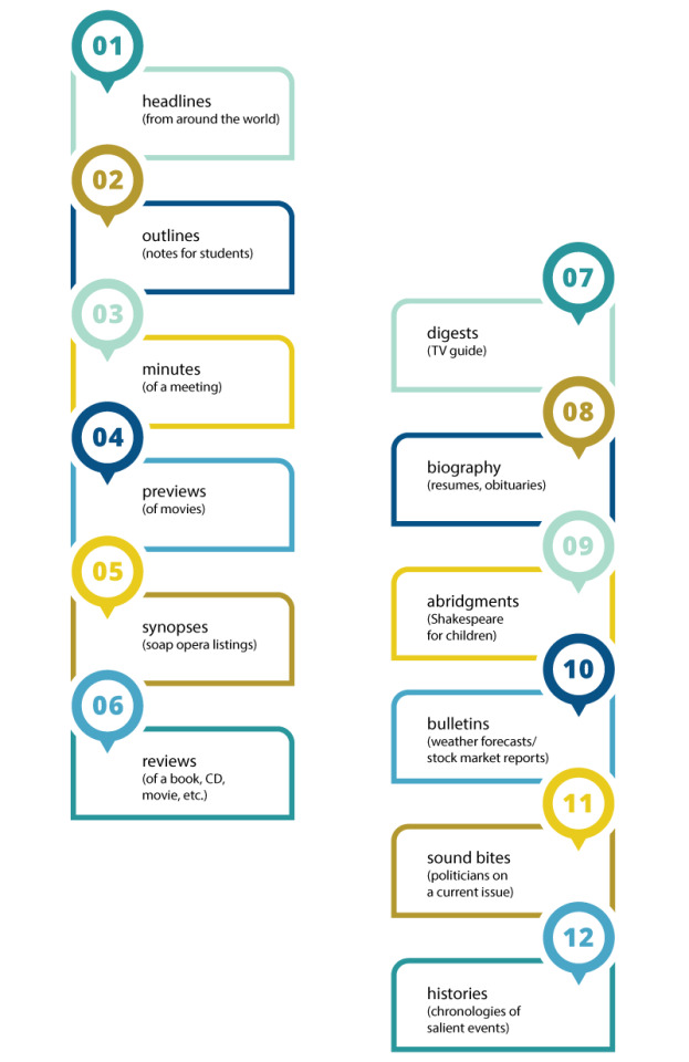
By now, the whole branch of natural language processing dedicated to summarization emerged, covering a variety of tasks:

· headlines (from around the world);

· outlines (notes for students);

· minutes (of a meeting);

· previews (of movies);

· synopses (soap opera listings);

· reviews (of a book, CD, movie, etc.);

· digests (TV guide);

· biography (resumes, obituaries);

· abridgments (Shakespeare for children);

· bulletins (weather forecasts/stock market reports);

· sound bites (politicians on a current issue);

· histories (chronologies of salient events).

The approaches to text summarization vary depending on the number of input documents (single or multiple), purpose (generic, domain specific, or query-based) and output (extractive or abstractive).

Extractive summarization means identifying important sections of the text and generating them verbatim producing a subset of the sentences from the original text; while abstractive summarization reproduces important material in a new way after interpretation and examination of the text using advanced natural language techniques to generate a new shorter text that conveys the most critical information from the original one.

Obviously, abstractive summarization is more advanced and closer to human-like interpretation. Though it has more potential (and is generally more interesting for researchers and developers), so far the more traditional methods have proved to yield better results.

That is why in this blog post we’ll give a short overview of such traditional approaches that have beaten a path to advanced deep learning techniques.

By now, the core of all extractive summarizers is formed of three independent tasks:

1) Construction of an intermediate representation of the input text

There are two types of representation-based approaches: topic representation and indicator representation. Topic representation transforms the text into an intermediate representation and interpret the topic(s) discussed in the text. The techniques used for this differ in terms of their complexity, and are divided into frequency-driven approaches, topic word approaches, latent semantic analysis and Bayesian topic models. Indicator representation describes every sentence as a list of formal features (indicators) of importance such as sentence length, position in the document, having certain phrases, etc.

2) Scoring the sentences based on the representation

When the intermediate representation is generated, an importance score is assigned to each sentence. In topic representation approaches, the score of a sentence represents how well the sentence explains some of the most important topics of the text. In indicator representation, the score is computed by aggregating the evidence from different weighted indicators.

3) Selection of a summary comprising of a number of sentences

The summarizer system selects the top k most important sentences to produce a summary. Some approaches use greedy algorithms to select the important sentences and some approaches may convert the selection of sentences into an optimization problem where a collection of sentences is chosen, considering the constraint that it should maximize overall importance and coherency and minimize the redundancy.

Let’s have a closer look at the approaches we mentioned and outline the differences between them:

Topic Representation Approaches

Topic words

This common technique aims to identify words that describe the topic of the input document. An advance of the initial Luhn’s idea was to use log-likelihood ratio test to identify explanatory words known as the “topic signature”. Generally speaking, there are two ways to compute the importance of a sentence: as a function of the number of topic signatures it contains, or as the proportion of the topic signatures in the sentence. While the first method gives higher scores to longer sentences with more words, the second one measures the density of the topic words.

Frequency-driven approaches

This approach uses frequency of words as indicators of importance. The two most common techniques in this category are: word probability and TFIDF (Term Frequency Inverse Document Frequency). The probability of a word w is determined as the number of occurrences of the word, f (w), divided by the number of all words in the input (which can be a single document or multiple documents). Words with highest probability are assumed to represent the topic of the document and are included in the summary. TFIDF, a more sophisticated technique, assesses the importance of words and identifies very common words (that should be omitted from consideration) in the document(s) by giving low weights to words appearing in most documents. TFIDF has given way to centroid-based approaches that rank sentences by computing their salience using a set of features. After creation of TFIDF vector representations of documents, the documents that describe the same topic are clustered together and centroids are computed — pseudo-documents that consist of the words whose TFIDF scores are higher than a certain threshold and form the cluster. Afterwards, the centroids are used to identify sentences in each cluster that are central to the topic.

Latent Semantic Analysis

Latent semantic analysis (LSA) is an unsupervised method for extracting a representation of text semantics based on observed words. The first step is to build a term-sentence matrix, where each row corresponds to a word from the input (n words) and each column corresponds to a sentence. Each entry of the matrix is the weight of the word i in sentence j computed by TFIDF technique. Then singular value decomposition (SVD) is used on the matrix that transforms the initial matrix into three matrices: a term-topic matrix having weights of words, a diagonal matrix where each row corresponds to the weight of a topic, and a topic-sentence matrix. If you multiply the diagonal matrix with weights with the topic-sentence matrix, the result will describe how much a sentence represent a topic, in other words, the weight of the topic i in sentence j.

Discourse Based Method

A logical development of analyzing semantics, is perform discourse analysis, finding the semantic relations between textual units, to form a summary. The study on cross-document relations was initiated by Radev, who came up withCross-Document Structure Theory (CST) model. In his model, words, phrases or sentences can be linked with each other if they are semantically connected. CST was indeed useful for document summarization to determine sentence relevance as well as to treat repetition, complementarity and inconsistency among the diverse data sources. Nonetheless, the significant limitation of this method is that the CST relations should be explicitly determined by human.

Bayesian Topic Models

While other approaches do not have very clear probabilistic interpretations, Bayesian topic models are probabilistic models that thanks to their describing topics in more detail can represent the information that is lost in other approaches. In topic modeling of text documents, the goal is to infer the words related to a certain topic and the topics discussed in a certain document, based on the prior analysis of a corpus of documents. It is possible with the help of Bayesian inference that calculates the probability of an event based on a combination of common sense assumptions and the outcomes of previous related events. The model is constantly improved by going through many iterations where a prior probability is updated with observational evidence to produce a new posterior probability.

Indicator representation approaches

The second large group of techniques aims to represent the text based on a set of features and use them to directly rank the sentences without representing the topics of the input text.

Graph Methods

Influenced by PageRank algorithm, these methods represent documents as a connected graph, where sentences form the vertices and edges between the sentences indicate how similar the two sentences are. The similarity of two sentences is measured with the help of cosine similarity with TFIDF weights for words and if it is greater than a certain threshold, these sentences are connected. This graph representation results in two outcomes: the sub-graphs included in the graph create topics covered in the documents, and the important sentences are identified. Sentences that are connected to many other sentences in a sub-graph are likely to be the center of the graph and will be included in the summary Since this method do not need language-specific linguistic processing, it can be applied to various languages [43]. At the same time, such measuring only of the formal side of the sentence structure without the syntactic and semantic information limits the application of the method.

Machine Learning

Machine learning approaches that treat summarization as a classification problem are widely used now trying to apply Naive Bayes, decision trees, support vector machines, Hidden Markov models and Conditional Random Fields to obtain a true-to-life summary. As it has turned out, the methods explicitly assuming the dependency between sentences (Hidden Markov model and Conditional Random Fields) often outperform other techniques.

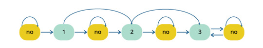
Figure 1: Summary Extraction Markov Model to Extract 2 Lead Sentences and Additional Supporting Sentences

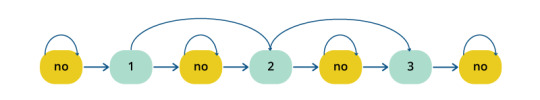
Figure 2: Summary Extraction Markov Model to Extract 3 Sentences

Yet, the problem with classifiers is that if we utilize supervised learning methods for summarization, we need a set of labeled documents to train the classifier, meaning development of a corpus. A possible way-out is to apply semi-supervised approaches that combine a small amount of labeled data along with a large amount of unlabeled data in training.

Overall, machine learning methods have proved to be very effective and successful both in single and multi-document summarization, especially in class-specific summarization such as drawing scientific paper abstracts or biographical summaries.

Though abundant, all the summarization methods we have mentioned could not produce summaries that would similar to human-created summaries. In many cases, the soundness and readability of created summaries are not satisfactory, because they fail to cover all the semantically relevant aspects of data in an effective way and afterwards they fail to connect sentences in a natural way.

In our next post, we’ll talk more about ways to overcome these problems and new approaches and techniques that have recently appeared in the field.

[s-c-i-guy]

A New Path to Equal-Angle Lines

Equiangular lines are an elemental part of geometry. Mathematicians have discovered a tighter limit on the number of such lines that exist in every dimension.

Imagine a set of many lines as in a dream. The lines intersect at a point and radiate outward. There’s something perfect about the way they’re spaced that you can’t quite put your finger on. You start counting them, but before you can finish you wake up with a question hanging on the fringe of your mind: Just how many were there?

For at least 70 years, mathematicians have been trying to answer a question like that one. The sets of lines they’re interested in share a basic feature: Any two lines from the set intersect to form the same angle. Such sets of lines are called “equiangular.” Mathematicians want to know just how big those sets can get as you move past the 3-D space of our everyday experience and into higher dimensions.

Equiangular lines are much more than a curiosity — they’re an almost elemental way to think about geometry. Maximal constructions of equiangular lines often align perfectly with the vertices of highly symmetric shapes, which make them a way to discover the existence of those shapes in the first place. In addition, radiating equiangular lines would pass through the surface of a surrounding sphere at equidistant points. This property makes the lines important for so-called spherical codes, which have important applications in applied mathematics and computer science.

Last spring a team of mathematicians found the maximum number of equiangular lines possible in any dimension, given certain conditions. They proved that that number is much smaller than previous best estimates. Benny Sudakov, a professor of mathematics at the Swiss Federal Institute of Technology Zurich and one of the lead authors, credits the breakthrough to the wide range of mathematical techniques he and his coauthors were able to apply to the problem.

“It’s like when you’re cooking something, we suddenly found we had the right ingredients,” said Sudakov.

To achieve the proof, the mathematicians figured out how to translate the problem into very different mathematical settings. The mathematicians were able to establish properties of equiangular lines in these translated forms that they then carried back into the geometric setting, almost in the way you might retrace your steps to a vision in a dream.

Lines in Many Forms

In simple cases, equiangular lines are easy to spot. In two dimensions, take a hexagon and connect opposite vertices. In the resulting construction, any pair of the three lines forms a 60-degree angle. In three dimensions, connecting opposite vertices of an icosahedron (a 3-D shape with 20 faces and 12 vertices) gives you six intersecting lines, any pair of which forms a 63.4-degree angle.

In more than three dimensions, it’s impossible to actually visualize what constructions of equiangular lines would look like, which is one reason it’s been hard to figure out the maximum number of equiangular lines in spaces of any dimension. The best that mathematicians have been able to do is prove that the number of equiangular lines can’t exceed roughly the square of the number of dimensions. (The exact upper bound for dimension d is (d2 + d)/2.) In most dimensions, they know that the number of possible lines is smaller than that.

Sudakov’s interest in equiangular constructions began in 2015 at a talk given by Boris Bukh, a mathematician at Carnegie Mellon University who’d recently made progress on a refined version of the problem. Bukh had proved that when you specify the size of the angle ahead of time — that is, you ask, what is the maximum number of equiangular lines with, say, a 50-degree angle between any pair of them — the maximum number of equiangular lines is much smaller than the known bound. Instead, it grows in linear fashion, as some constant times the number of dimensions.

Bukh’s result wasn’t elegant — “It wasn’t the best approach in some sense,’’ he said. “I did some ugly things to make my proof work” — but it got Sudakov thinking about the problem. That same year Sudakov spent a semester at the University of Oxford, where he talked through potential lines of attack with Peter Keevash, a mathematician there. Sudakov then returned to Zurich and shared his emerging ideas with his graduate students Igor Balla and Felix Dräxler. They made a suggestion of their own, and suddenly the way to prove a tighter bound on the number of equiangular lines with a specified angle seemed clear. “We all started working on it frantically,” Sudakov said.

Their method was not so different, in spirit, from the way scientists hunt for signatures of an event they can’t observe — they look for traces of the event in other forms. The mathematicians pictured a set of some number of equiangular lines with a specified angle. If the lines were to exist, they could also be represented as other kinds of mathematical objects. The mathematicians proceeded to examine the properties of these analogous objects, knowing that once they understood them, they could work backward from there to the lines themselves.

To see the steps in this approach, it’s helpful to think about how you get from the lines to the analogous objects, even though the actual construction of the lines proceeds in the opposite direction.

Take a set of equiangular lines. Associate to each line a vector — an object that points in a particular direction. For each line you can imagine two possible vectors, one pointing one way on the line, the other pointing the other way. Choose one, then take the “dot product” of each pair of vectors. If the vectors form an acute angle, the dot product will be positive. If they form an obtuse angle, it will be negative.

The major innovations in the new work appeared after the authors recast the problem in the language of graph theory. Graph theory is the study of how points can be connected to each other by edges. In this scenario, the points of the graph represent the vectors. Points are connected to each other according to this rule: Color the edge between them red if the dot product is positive, blue if the dot product is negative. The result will be a configuration of red and blue lines that provides a different way of looking at the original situation.

“This is another way of encoding the information you’re given, but it’s quite suggestive,” said Keevash. “Once you have a graph, combinatorial ideas come into play.”

In particular, the authors use something called Ramsey’s theorem to bring order to the way all the red and blue edges are joined together. Ramsey’s theorem says that a graph of this sort will always contain large subsets of a certain minimum size that are completely uniform — either all red or all blue. In the case at hand, we know it’s impossible to have many vectors pointing in opposite directions, so the dominant subset of lines will always be red, not blue.

This large subset of red edges forms what Sudakov calls an “anchor” from which he and his collaborators are able to fill out the rest of the graph. By manipulating the remaining vectors, they prove that almost all the vectors not in the subset are joined to the subset via red edges. This, in a sense, casts the blue edges to the outskirts of the graph, and gives the authors a complete, well-ordered picture of what a graphical representation of a set of equiangular lines would look like — if those lines were to exist.

The authors took this arrangement of vectors and further simplified the picture by “projecting” it down into lower dimensions, where additional aspects of their structure came into view.

“It’s a bit like taking a light and shining it on an object and looking at the shadow,” said Jonathan Jedwab, a mathematician at Simon Fraser University in British Columbia who studies equiangular lines. “If you have a three-dimensional object and literally shine a light on it, the shadow it casts on the two-dimensional plane will tell something about what’s going on. If you then moved the 3-D object and shone the light again you could compare the 2-D shadows and learn even more.”

Following the projection, the authors changed settings one final time, reinterpreting their graph as a matrix — a square table of entries. In this table, each entry is a dot product of two vectors. Mathematicians commonly use these kinds of matrices — called Gram matrices — to study configurations of vectors, and in particular those coming from equiangular lines. In this new work, though, the authors had the advantage of first having used Ramsey’s theorem to understand something about the structure of vector relationships.

“After identifying this set, suddenly we cleaned the whole picture and the matrices we got later were much more structured,” said Sudakov.

Through a variety of manipulations, the researchers calculated the “rank” of these structured matrices. Rank is a basic attribute of any matrix. It quantifies, in a sense, how much information the matrix contains, or how many rows you need in order to be able to generate all the rows. (A rough analog of rank would be to count the number of primes needed to express the prime factorization of a number — a number with a longer prime factorization would be considered more complex and have a higher “rank.”)

In this setup, the rank of the matrix is both related to the number of equiangular lines and sets a limit on the number of spatial dimensions in which the lines live. As a result, the authors were able to prove that when you begin by fixing the angle in advance, the maximum number of equiangular lines is 2d – 2 for one particular angle (approximately 70.7 degrees), and no more than 1.93d for any other angle. The authors ended up needing a roundabout process to arrive at such exact numbers, but sometimes it takes a surprising series of recollections to find your way back to last night’s dream.

“My reaction isn’t ‘Why didn’t I think of it?’ It’s ‘My goodness, what an array of tools these people have,’” said Jedwab. “To string these tools together one after another, I think that’s the real ingeniousness of what they’ve done.”

[angeeroachus]

[Packt] Implementing Graph Algorithms Using Scala [Integrated Course]

Learn functional programming in Scala by implementing various graph algorithms Video Description Scala's functional programming features are a boon to help you design “easy to reason about” systems to control growing software complexities.In this course we practise many functional techniques by solving various graph problems. We start by looking at how we can represent graph structures in an efficient functional manner. Then we explore both the breadth and depth first search graph traversal techniques. Later we use this techniques to show how they can be used for topological sorting and cycle detection. In this course we also describe more complex algorithms such as finding the shortest path and maximal flow networks. All of these solutions are illustrated with easy to understand diagrams and animations. Special care is taken when writing solution so that the principles of functional programming are followed. By the end of the course, you will be well-versed in all the functional concepts of Scala and you will have refreshed your knowledge of graph algorithms. The code and supporting files for the course are available at https://github.com/PacktPublishing/Implementing-Graph-Algorithms-using-Scala Style and Approach The course starts off with explaining the basic graph algorithms. We discuss each algorithm briefly before proceeding to implement it in Scala. This way, you understand not only the functional implementation, but also the underlying concepts behind the algorithm. What You Will Learn Understand adjacency list and matrix representation Learn BFS vs DFS graph traversal and the implemented in a functional manner Implement a topological sort algorithm Discover how to implement a cycle detection in graphs. Understand and develop the existing Dijkstra's shortest path algorithm, Understand what is max flow in a flow network and implement the Ford-Fulkerson method and the Edmonds-Karp algorithm Authors James Cutajar James Cutajar is a software developer with interests in scalable, high-performance computing and distributed algorithms. He is also an open source contributor, author, blogger, and tech evangelist. When he is not writing software, he is riding his motorbike, surfing, or flying light aircraft. He was born in Malta, lived for almost a decade in London, and is now working in Portugal. source https://ttorial.com/implementing-graph-algorithms-using-scala-integrated-course

[ianasennus]

[Packt] Implementing Graph Algorithms Using Scala [Integrated Course]

Learn functional programming in Scala by implementing various graph algorithms Video Description Scala’s functional programming features are a boon to help you design “easy to reason about” systems to control growing software complexities.In this course we practise many functional techniques by solving various graph problems. We start by looking at how we can represent graph structures in an efficient functional manner. Then we explore both the breadth and depth first search graph traversal techniques. Later we use this techniques to show how they can be used for topological sorting and cycle detection. In this course we also describe more complex algorithms such as finding the shortest path and maximal flow networks. All of these solutions are illustrated with easy to understand diagrams and animations. Special care is taken when writing solution so that the principles of functional programming are followed. By the end of the course, you will be well-versed in all the functional concepts of Scala and you will have refreshed your knowledge of graph algorithms. The code and supporting files for the course are available at https://github.com/PacktPublishing/Implementing-Graph-Algorithms-using-Scala Style and Approach The course starts off with explaining the basic graph algorithms. We discuss each algorithm briefly before proceeding to implement it in Scala. This way, you understand not only the functional implementation, but also the underlying concepts behind the algorithm. What You Will Learn Understand adjacency list and matrix representation Learn BFS vs DFS graph traversal and the implemented in a functional manner Implement a topological sort algorithm Discover how to implement a cycle detection in graphs. Understand and develop the existing Dijkstra’s shortest path algorithm, Understand what is max flow in a flow network and implement the Ford-Fulkerson method and the Edmonds-Karp algorithm Authors James Cutajar James Cutajar is a software developer with interests in scalable, high-performance computing and distributed algorithms. He is also an open source contributor, author, blogger, and tech evangelist. When he is not writing software, he is riding his motorbike, surfing, or flying light aircraft. He was born in Malta, lived for almost a decade in London, and is now working in Portugal. source https://ttorial.com/implementing-graph-algorithms-using-scala-integrated-course

source https://ttorialcom.tumblr.com/post/176295710738

[ttorialcom]

[Packt] Implementing Graph Algorithms Using Scala [Integrated Course]

Learn functional programming in Scala by implementing various graph algorithms Video Description Scala's functional programming features are a boon to help you design “easy to reason about” systems to control growing software complexities.In this course we practise many functional techniques by solving various graph problems. We start by looking at how we can represent graph structures in an efficient functional manner. Then we explore both the breadth and depth first search graph traversal techniques. Later we use this techniques to show how they can be used for topological sorting and cycle detection. In this course we also describe more complex algorithms such as finding the shortest path and maximal flow networks. All of these solutions are illustrated with easy to understand diagrams and animations. Special care is taken when writing solution so that the principles of functional programming are followed. By the end of the course, you will be well-versed in all the functional concepts of Scala and you will have refreshed your knowledge of graph algorithms. The code and supporting files for the course are available at https://github.com/PacktPublishing/Implementing-Graph-Algorithms-using-Scala Style and Approach The course starts off with explaining the basic graph algorithms. We discuss each algorithm briefly before proceeding to implement it in Scala. This way, you understand not only the functional implementation, but also the underlying concepts behind the algorithm. What You Will Learn Understand adjacency list and matrix representation Learn BFS vs DFS graph traversal and the implemented in a functional manner Implement a topological sort algorithm Discover how to implement a cycle detection in graphs. Understand and develop the existing Dijkstra's shortest path algorithm, Understand what is max flow in a flow network and implement the Ford-Fulkerson method and the Edmonds-Karp algorithm Authors James Cutajar James Cutajar is a software developer with interests in scalable, high-performance computing and distributed algorithms. He is also an open source contributor, author, blogger, and tech evangelist. When he is not writing software, he is riding his motorbike, surfing, or flying light aircraft. He was born in Malta, lived for almost a decade in London, and is now working in Portugal. source https://ttorial.com/implementing-graph-algorithms-using-scala-integrated-course