#pd.merge
Explore tagged Tumblr posts
Visit Tumblr Blog
Explore Tumblr blogs with no restrictions, modern design and the best experience.
Last Seen Tumblr Blogs


Fun Fact
12.7% of mobile users access Tumblr.
Text
SVERWEIS() oder XVERWEIS() mit Python in Excel durchführen
In der heutigen Excel-Welt wird die Zusammenführung von Daten mithilfe von SVERWEIS() oder XVERWEIS() als selbstverständlich angesehen. Aber wussten Sie, dass Sie diese Aufgabe auch problemlos in Python mit pd.merge erledigen können? In diesem Artikel werfen wir einen Blick auf die Grundlagen der Verwendung von pd.merge in Python, um Daten miteinander zu verknüpfen. Hierzu wurde ein interessantes…

View On WordPress
0 notes
Text
K-means clusthering
#importamos las librerías necesarias
from pandas import Series,DataFrame
import pandas as pd
import numpy as np
import matplotlib.pylab as plt
from sklearn.model_selection
import train_test_splitfrom sklearn
import preprocessing
from sklearn.cluster import KMeans
"""Data Management"""
data =pd.read_csv("/content/drive/MyDrive/tree_addhealth.csv" )
#upper-case all DataFrame column names
data.columns = map(str.upper, data.columns)
# Data Managementdata_clean = data.dropna()
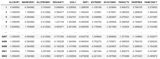
# subset clustering variablescluster=data_clean[['ALCEVR1','MAREVER1','ALCPROBS1','DEVIANT1','VIOL1','DEP1','ESTEEM1','SCHCONN1','PARACTV', 'PARPRES','FAMCONCT']]
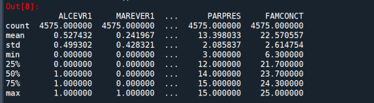
cluster.describe()
# standardize clustering variables to have mean=0 and sd=1
clustervar=cluster.copy()
clustervar['ALCEVR1']=preprocessing.scale(clustervar['ALCEVR1'].astype('float64'))
clustervar['ALCPROBS1']=preprocessing.scale(clustervar['ALCPROBS1'].astype('float64'))
clustervar['MAREVER1']=preprocessing.scale(clustervar['MAREVER1'].astype('float64'))
clustervar['DEP1']=preprocessing.scale(clustervar['DEP1'].astype('float64'))
clustervar['ESTEEM1']=preprocessing.scale(clustervar['ESTEEM1'].astype('float64'))
clustervar['VIOL1']=preprocessing.scale(clustervar['VIOL1'].astype('float64'))
clustervar['DEVIANT1']=preprocessing.scale(clustervar['DEVIANT1'].astype('float64'))
clustervar['FAMCONCT']=preprocessing.scale(clustervar['FAMCONCT'].astype('float64'))
clustervar['SCHCONN1']=preprocessing.scale(clustervar['SCHCONN1'].astype('float64'))
clustervar['PARACTV']=preprocessing.scale(clustervar['PARACTV'].astype('float64'))
clustervar['PARPRES']=preprocessing.scale(clustervar['PARPRES'].astype('float64'))
# split data into train and test sets
clus_train, clus_test = train_test_split(clustervar, test_size=.3, random_state=123)
# k-means cluster analysis for 1-9 clusters
from scipy.spatial.distance import cdist
clusters=range(1,10)
meandist=[]
for k in clusters: model=KMeans(n_clusters=k) model.fit(clus_train) clusassign=model.predict(clus_train) meandist.append(sum(np.min(cdist(clus_train, model.cluster_centers_, 'euclidean'), axis=1))
/ clus_train.shape[0])
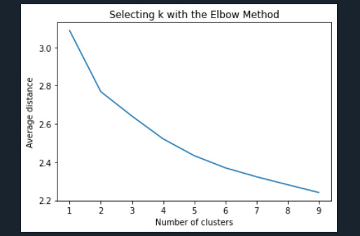
"""Plot average distance from observations from the cluster centroidto use the Elbow Method to identify number of clusters to choose"""
plt.plot(clusters,meandist)
plt.xlabel('Number of clusters')
plt.ylabel('Average distance')
plt.title('Selecting k with the Elbow Method')
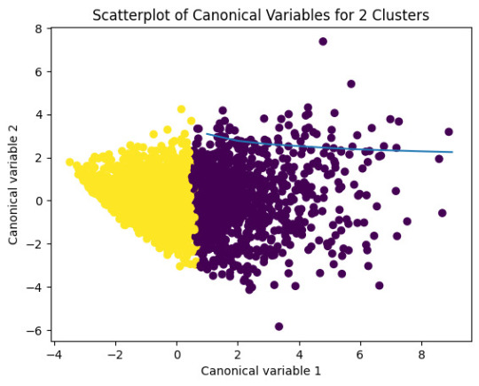
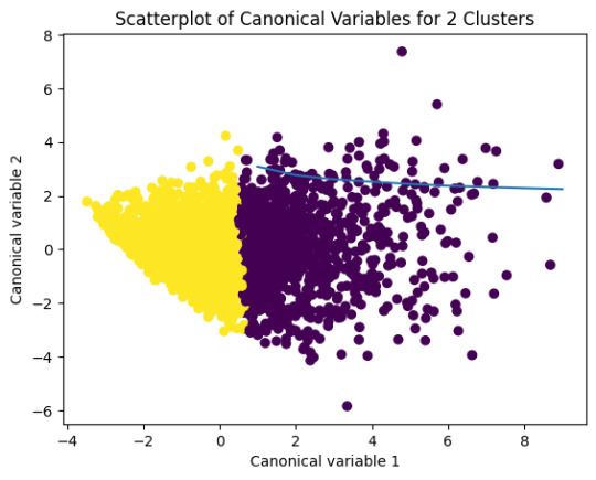
# Interpret 2 cluster solution
model2=KMeans(n_clusters=2)model2.fit(clus_train)
clusassign=model2.predict(clus_train)
# plot clusters
from sklearn.decomposition import PCA
pca_2 = PCA(2)
plot_columns = pca_2.fit_transform(clus_train)
plt.scatter(x=plot_columns[:,0],y=plot_columns[:,1],c=model2.labels_,)
plt.xlabel('Canonical variable 1')
plt.ylabel('Canonical variable 2')
plt.title('Scatterplot of Canonical Variables for 2 Clusters')
plt.show()
"""BEGIN multiple steps to merge cluster assignment with clustering variables to examinecluster variable means by cluster"""
# create a unique identifier variable from the index for the
# cluster training data to merge with the cluster assignment variable
clus_train.reset_index(level=0, inplace=True)
# create a list that has the new index variable
cluslist=list(clus_train['index'])
# create a list of cluster assignments
labels=list(model2.labels_)
# combine index variable list with cluster assignment list into a dictionary
newlist=dict(zip(cluslist, labels))newlist
# convert newlist dictionary to a dataframenew
clus=DataFrame.from_dict(newlist, orient='index')newclus
# rename the cluster assignment columnnew
clus.columns = ['cluster']
# now do the same for the cluster assignment variable
# create a unique identifier variable from the index for the
# cluster assignment dataframe
# to merge with cluster training datanew
clus.reset_index(level=0, inplace=True)
# merge the cluster assignment dataframe with the cluster training variable dataframe
# by the index variablemerged_train=pd.merge(clus_train, newclus, on='index')
merged_train.head(n=100)
# cluster frequenciesmerged_train.cluster.value_counts()
"""END multiple steps to merge cluster assignment with clustering variables to examinecluster variable means by cluster"""
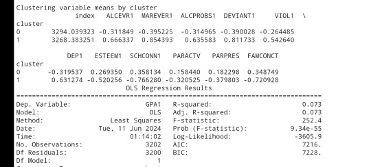
# FINALLY calculate clustering variable means by
clusterclustergrp = merged_train.groupby('cluster').mean()print ("Clustering variable means by cluster")
print(clustergrp)
# validate clusters in training data by examining cluster differences in GPA using ANOVA
# first have to merge GPA with clustering variables and cluster assignment data
gpa_data=data_clean['GPA1']
# split GPA data into train and test sets
gpa_train, gpa_test = train_test_split(gpa_data, test_size=.3, random_state=123)
gpa_train1=pd.DataFrame(gpa_train)
gpa_train1.reset_index(level=0, inplace=True)
merged_train_all=pd.merge(gpa_train1, merged_train, on='index')
sub1 = merged_train_all[['GPA1', 'cluster']].dropna()
import statsmodels.formula.api as smf
import statsmodels.stats.multicomp as multi
gpamod = smf.ols(formula='GPA1 ~ C(cluster)', data=sub1).fit()
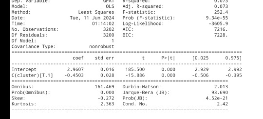
print (gpamod.summary())
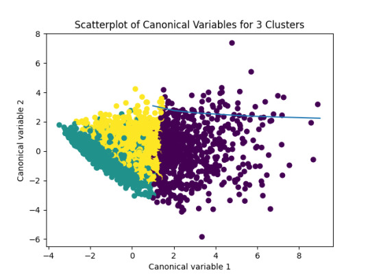
print ('means for GPA by cluster')
m1= sub1.groupby('cluster').mean()
print (m1)
print ('standard deviations for GPA by cluster')
m2= sub1.groupby('cluster').std()print (m2)
mc1 = multi.MultiComparison(sub1['GPA1'], sub1['cluster'])
res1 = mc1.tukeyhsd()
print(res1.summary())
爆發
0 則迴響
0 notes
Text
K-means clusthering
#importamos las librerías necesarias
from pandas import Series,DataFrame
import pandas as pd
import numpy as np
import matplotlib.pylab as plt
from sklearn.model_selection
import train_test_splitfrom sklearn
import preprocessing
from sklearn.cluster import KMeans
"""Data Management"""
data =pd.read_csv("/content/drive/MyDrive/tree_addhealth.csv" )
#upper-case all DataFrame column names
data.columns = map(str.upper, data.columns)
# Data Managementdata_clean = data.dropna()
# subset clustering variablescluster=data_clean[['ALCEVR1','MAREVER1','ALCPROBS1','DEVIANT1','VIOL1','DEP1','ESTEEM1','SCHCONN1','PARACTV', 'PARPRES','FAMCONCT']]
cluster.describe()
# standardize clustering variables to have mean=0 and sd=1
clustervar=cluster.copy()
clustervar['ALCEVR1']=preprocessing.scale(clustervar['ALCEVR1'].astype('float64'))
clustervar['ALCPROBS1']=preprocessing.scale(clustervar['ALCPROBS1'].astype('float64'))
clustervar['MAREVER1']=preprocessing.scale(clustervar['MAREVER1'].astype('float64'))
clustervar['DEP1']=preprocessing.scale(clustervar['DEP1'].astype('float64'))
clustervar['ESTEEM1']=preprocessing.scale(clustervar['ESTEEM1'].astype('float64'))
clustervar['VIOL1']=preprocessing.scale(clustervar['VIOL1'].astype('float64'))
clustervar['DEVIANT1']=preprocessing.scale(clustervar['DEVIANT1'].astype('float64'))
clustervar['FAMCONCT']=preprocessing.scale(clustervar['FAMCONCT'].astype('float64'))
clustervar['SCHCONN1']=preprocessing.scale(clustervar['SCHCONN1'].astype('float64'))
clustervar['PARACTV']=preprocessing.scale(clustervar['PARACTV'].astype('float64'))
clustervar['PARPRES']=preprocessing.scale(clustervar['PARPRES'].astype('float64'))
# split data into train and test sets
clus_train, clus_test = train_test_split(clustervar, test_size=.3, random_state=123)
# k-means cluster analysis for 1-9 clusters
from scipy.spatial.distance import cdist
clusters=range(1,10)
meandist=[]
for k in clusters: model=KMeans(n_clusters=k) model.fit(clus_train) clusassign=model.predict(clus_train) meandist.append(sum(np.min(cdist(clus_train, model.cluster_centers_, 'euclidean'), axis=1))
/ clus_train.shape[0])
"""Plot average distance from observations from the cluster centroidto use the Elbow Method to identify number of clusters to choose"""
plt.plot(clusters,meandist)
plt.xlabel('Number of clusters')
plt.ylabel('Average distance')
plt.title('Selecting k with the Elbow Method')
# Interpret 2 cluster solution
model2=KMeans(n_clusters=2)model2.fit(clus_train)
clusassign=model2.predict(clus_train)
# plot clusters
from sklearn.decomposition import PCA
pca_2 = PCA(2)
plot_columns = pca_2.fit_transform(clus_train)
plt.scatter(x=plot_columns[:,0],y=plot_columns[:,1],c=model2.labels_,)
plt.xlabel('Canonical variable 1')
plt.ylabel('Canonical variable 2')
plt.title('Scatterplot of Canonical Variables for 2 Clusters')
plt.show()
"""BEGIN multiple steps to merge cluster assignment with clustering variables to examinecluster variable means by cluster"""
# create a unique identifier variable from the index for the
# cluster training data to merge with the cluster assignment variable
clus_train.reset_index(level=0, inplace=True)
# create a list that has the new index variable
cluslist=list(clus_train['index'])
# create a list of cluster assignments
labels=list(model2.labels_)
# combine index variable list with cluster assignment list into a dictionary
newlist=dict(zip(cluslist, labels))newlist
# convert newlist dictionary to a dataframenew
clus=DataFrame.from_dict(newlist, orient='index')newclus
# rename the cluster assignment columnnew
clus.columns = ['cluster']
# now do the same for the cluster assignment variable
# create a unique identifier variable from the index for the
# cluster assignment dataframe
# to merge with cluster training datanew
clus.reset_index(level=0, inplace=True)
# merge the cluster assignment dataframe with the cluster training variable dataframe
# by the index variablemerged_train=pd.merge(clus_train, newclus, on='index')
merged_train.head(n=100)
# cluster frequenciesmerged_train.cluster.value_counts()
"""END multiple steps to merge cluster assignment with clustering variables to examinecluster variable means by cluster"""
# FINALLY calculate clustering variable means by
clusterclustergrp = merged_train.groupby('cluster').mean()print ("Clustering variable means by cluster")
print(clustergrp)
# validate clusters in training data by examining cluster differences in GPA using ANOVA
# first have to merge GPA with clustering variables and cluster assignment data
gpa_data=data_clean['GPA1']
# split GPA data into train and test sets
gpa_train, gpa_test = train_test_split(gpa_data, test_size=.3, random_state=123)
gpa_train1=pd.DataFrame(gpa_train)
gpa_train1.reset_index(level=0, inplace=True)
merged_train_all=pd.merge(gpa_train1, merged_train, on='index')
sub1 = merged_train_all[['GPA1', 'cluster']].dropna()
import statsmodels.formula.api as smf
import statsmodels.stats.multicomp as multi
gpamod = smf.ols(formula='GPA1 ~ C(cluster)', data=sub1).fit()
print (gpamod.summary())
print ('means for GPA by cluster')
m1= sub1.groupby('cluster').mean()
print (m1)
print ('standard deviations for GPA by cluster')
m2= sub1.groupby('cluster').std()print (m2)
mc1 = multi.MultiComparison(sub1['GPA1'], sub1['cluster'])
res1 = mc1.tukeyhsd()
print(res1.summary())
0 notes
Text
Merging in Data Analyst
Data Analyst Course Online, Merging, or data merging, is a critical process in data analysis where multiple datasets are combined to create a unified and comprehensive dataset. This is often necessary because data may be collected and stored in different sources or formats. Here's an overview of data merging in data analysis:
Why Data Merging is Important:
Completeness: Merging data from various sources can help fill gaps and provide a more complete picture of the phenomenon or topic being studied.
Enrichment: Combining different datasets can enhance the information available for analysis by adding new variables or dimensions.
Comparative Analysis: Merging allows for the comparison of data from different sources, such as sales data from multiple regions or years.
Common Methods of Data Merging:
Joining: In relational databases and tools like SQL, merging is often achieved through joins. Common join types include inner join, left join, right join, and full outer join. These operations link rows in one dataset with rows in another based on a specified key or common attribute.
Concatenation: When merging datasets with the same structure vertically, concatenation is used. This is common in scenarios where data is collected over time and stored in separate files or tables.
Merging in Statistical Software: Tools like R and Python offer functions (e.g., merge() in R or pd.merge() in Python) that facilitate dataset merging based on specified keys or columns.
Data Integration Tools: For large and complex data integration tasks, specialized data integration tools and platforms are available, which offer more advanced capabilities for data merging and transformation.
Challenges in Data Merging:
Data Consistency: Inconsistent data formats, missing values, or conflicting information across datasets can pose challenges during merging.
Data Quality: Data quality issues in one dataset can affect the quality of the merged dataset, making data cleaning and preprocessing crucial.
Key Identification: Identifying the correct keys or columns to merge datasets is essential. Choosing the wrong key can result in incorrect merging.
Data Volume: Merging large datasets can be computationally intensive and may require efficient techniques to handle memory and performance constraints.
Data merging is a fundamental step in data analysis, as it allows analysts to work with a more comprehensive dataset that can yield deeper insights and support informed decision-making. However, it requires careful planning, data preparation, and attention to data quality to ensure accurate and meaningful results.
0 notes
Text
rom pandas import Series, DataFrame import pandas as pd import numpy as np import matplotlib.pylab as plt from sklearn.model_selection import train_test_split from sklearn import preprocessing from sklearn.cluster import KMeans
""" Data Management """ data = pd.read_csv("tree_addhealth")
upper-case all DataFrame column names
data.columns = map(str.upper, data.columns)
Data Management
data_clean = data.dropna()
subset clustering variables
cluster=data_clean[['ALCEVR1','MAREVER1','ALCPROBS1','DEVIANT1','VIOL1', 'DEP1','ESTEEM1','SCHCONN1','PARACTV', 'PARPRES','FAMCONCT']] cluster.describe()
standardize clustering variables to have mean=0 and sd=1
clustervar=cluster.copy() clustervar['ALCEVR1']=preprocessing.scale(clustervar['ALCEVR1'].astype('float64')) clustervar['ALCPROBS1']=preprocessing.scale(clustervar['ALCPROBS1'].astype('float64')) clustervar['MAREVER1']=preprocessing.scale(clustervar['MAREVER1'].astype('float64')) clustervar['DEP1']=preprocessing.scale(clustervar['DEP1'].astype('float64')) clustervar['ESTEEM1']=preprocessing.scale(clustervar['ESTEEM1'].astype('float64')) clustervar['VIOL1']=preprocessing.scale(clustervar['VIOL1'].astype('float64')) clustervar['DEVIANT1']=preprocessing.scale(clustervar['DEVIANT1'].astype('float64')) clustervar['FAMCONCT']=preprocessing.scale(clustervar['FAMCONCT'].astype('float64')) clustervar['SCHCONN1']=preprocessing.scale(clustervar['SCHCONN1'].astype('float64')) clustervar['PARACTV']=preprocessing.scale(clustervar['PARACTV'].astype('float64')) clustervar['PARPRES']=preprocessing.scale(clustervar['PARPRES'].astype('float64'))
split data into train and test sets
clus_train, clus_test = train_test_split(clustervar, test_size=.3, random_state=123)
k-means cluster analysis for 1-9 clusters
from scipy.spatial.distance import cdist clusters=range(1,10) meandist=[]
for k in clusters: model=KMeans(n_clusters=k) model.fit(clus_train) clusassign=model.predict(clus_train) meandist.append(sum(np.min(cdist(clus_train, model.cluster_centers_, 'euclidean'), axis=1)) / clus_train.shape[0])
""" Plot average distance from observations from the cluster centroid to use the Elbow Method to identify number of clusters to choose """
plt.plot(clusters, meandist) plt.xlabel('Number of clusters') plt.ylabel('Average distance') plt.title('Selecting k with the Elbow Method')
Interpret 3 cluster solution
model3=KMeans(n_clusters=3) model3.fit(clus_train) clusassign=model3.predict(clus_train)
plot clusters
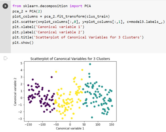
from sklearn.decomposition import PCA pca_2 = PCA(2) plot_columns = pca_2.fit_transform(clus_train) plt.scatter(x=plot_columns[:,0], y=plot_columns[:,1], c=model3.labels_,) plt.xlabel('Canonical variable 1') plt.ylabel('Canonical variable 2') plt.title('Scatterplot of Canonical Variables for 3 Clusters') plt.show()
""" BEGIN multiple steps to merge cluster assignment with clustering variables to examine cluster variable means by cluster """
create a unique identifier variable from the index for the
cluster training data to merge with the cluster assignment variable
clus_train.reset_index(level=0, inplace=True)
create a list that has the new index variable
cluslist=list(clus_train['index'])
create a list of cluster assignments
labels=list(model3.labels_)
combine index variable list with cluster assignment list into a dictionary
newlist=dict(zip(cluslist, labels)) newlist
convert newlist dictionary to a dataframe
newclus=DataFrame.from_dict(newlist, orient='index') newclus
rename the cluster assignment column
newclus.columns = ['cluster']
now do the same for the cluster assignment variable
create a unique identifier variable from the index for the
cluster assignment dataframe
to merge with cluster training data
newclus.reset_index(level=0, inplace=True)
merge the cluster assignment dataframe with the cluster training variable dataframe
by the index variable
merged_train=pd.merge(clus_train, newclus, on='index') merged_train.head(n=100)
cluster frequencies
merged_train.cluster.value_counts()
""" END multiple steps to merge cluster assignment with clustering variables to examine cluster variable means by cluster """
FINALLY calculate clustering variable means by cluster
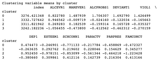
clustergrp = merged_train.groupby('cluster').mean() print ("Clustering variable means by cluster") print(clustergrp)
validate clusters in training data by examining cluster differences in GPA using ANOVA
first have to merge GPA with clustering variables and cluster assignment data
gpa_data=data_clean['GPA1']
split GPA data into train and test sets
gpa_train, gpa_test = train_test_split(gpa_data, test_size=.3, random_state=123) gpa_train1=pd.DataFrame(gpa_train) gpa_train1.reset_index(level=0, inplace=True) merged_train_all=pd.merge(gpa_train1, merged_train, on='index') sub1 = merged_train_all[['GPA1', 'cluster']].dropna()
import statsmodels.formula.api as smf import statsmodels.stats.multicomp as multi
gpamod = smf.ols(formula='GPA1 ~ C(cluster)', data=sub1).fit() print (gpamod.summary())
print ('means for GPA by cluster') m1= sub1.groupby('cluster').mean() print (m1)
print ('standard deviations for GPA by cluster') m2= sub1.groupby('cluster').std() print (m2)
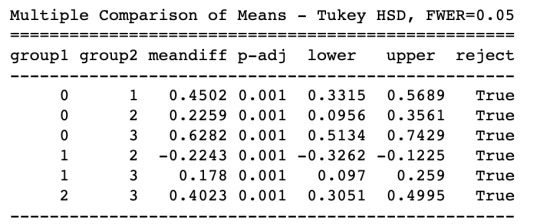
mc1 = multi.MultiComparison(sub1['GPA1'], sub1['cluster']) res1 = mc1.tukeyhsd() print(res1.summary())
0 notes
Text
K-Means Clustering
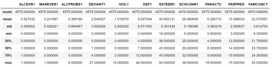
1. Data
I used the data "tree_addhealth.csv" for my coursera K-means assignment. This analysis was conducted in Python. The variables selected to perform the clustering data were:
cluster=data_clean[['ALCEVR1','MAREVER1','ALCPROBS1','DEVIANT1','VIOL1', 'DEP1','ESTEEM1','SCHCONN1','PARACTV', 'PARPRES','FAMCONCT']] cluster.describe()
2. Code
On the other hand, the code used to perform the analysis is the following: ---- START CODE ----
from pandas import Series, DataFrame import pandas as pd import numpy as np import matplotlib.pylab as plt from sklearn.model_selection import train_test_split from sklearn import preprocessing from sklearn.cluster import KMeans import os
os.chdir("../data/")
""" Data Management """ data = pd.read_csv("tree_addhealth.csv")
data.columns = map(str.upper, data.columns)
data_clean = data.dropna()
cluster=data_clean[['ALCEVR1','MAREVER1','ALCPROBS1','DEVIANT1','VIOL1', 'DEP1','ESTEEM1','SCHCONN1','PARACTV', 'PARPRES','FAMCONCT']] cluster.describe()
clustervar=cluster.copy() clustervar['ALCEVR1']=preprocessing.scale(clustervar['ALCEVR1'].astype('float64')) clustervar['ALCPROBS1']=preprocessing.scale(clustervar['ALCPROBS1'].astype('float64')) clustervar['MAREVER1']=preprocessing.scale(clustervar['MAREVER1'].astype('float64')) clustervar['DEP1']=preprocessing.scale(clustervar['DEP1'].astype('float64')) clustervar['ESTEEM1']=preprocessing.scale(clustervar['ESTEEM1'].astype('float64')) clustervar['VIOL1']=preprocessing.scale(clustervar['VIOL1'].astype('float64')) clustervar['DEVIANT1']=preprocessing.scale(clustervar['DEVIANT1'].astype('float64')) clustervar['FAMCONCT']=preprocessing.scale(clustervar['FAMCONCT'].astype('float64')) clustervar['SCHCONN1']=preprocessing.scale(clustervar['SCHCONN1'].astype('float64')) clustervar['PARACTV']=preprocessing.scale(clustervar['PARACTV'].astype('float64')) clustervar['PARPRES']=preprocessing.scale(clustervar['PARPRES'].astype('float64'))
clus_train, clus_test = train_test_split(clustervar, test_size=.3, random_state=123)
from scipy.spatial.distance import cdist clusters=range(1,10) meandist=[]
for k in clusters: model=KMeans(n_clusters=k) model.fit(clus_train) clusassign=model.predict(clus_train) meandist.append(sum(np.min(cdist(clus_train, model.cluster_centers_, 'euclidean'), axis=1)) / clus_train.shape[0])
""" Plot average distance from observations from the cluster centroid to use the Elbow Method to identify number of clusters to choose """
plt.plot(clusters, meandist) plt.xlabel('Number of clusters') plt.ylabel('Average distance') plt.title('Selecting k with the Elbow Method')
model3=KMeans(n_clusters=3) model3.fit(clus_train) clusassign=model3.predict(clus_train)
from sklearn.decomposition import PCA pca_2 = PCA(2) plot_columns = pca_2.fit_transform(clus_train) plt.scatter(x=plot_columns[:,0], y=plot_columns[:,1], c=model3.labels_,) plt.xlabel('Canonical variable 1') plt.ylabel('Canonical variable 2') plt.title('Scatterplot of Canonical Variables for 3 Clusters') plt.show()
""" BEGIN multiple steps to merge cluster assignment with clustering variables to examine cluster variable means by cluster """
clus_train.reset_index(level=0, inplace=True)
cluslist=list(clus_train['index'])
labels=list(model3.labels_)
newlist=dict(zip(cluslist, labels)) newlist
newclus=DataFrame.from_dict(newlist, orient='index') newclus
newclus.columns = ['cluster']
newclus.reset_index(level=0, inplace=True)
merged_train=pd.merge(clus_train, newclus, on='index') merged_train.head(n=100)
merged_train.cluster.value_counts()
""" END multiple steps to merge cluster assignment with clustering variables to examine cluster variable means by cluster """
clustergrp = merged_train.groupby('cluster').mean() print ("Clustering variable means by cluster") print(clustergrp)
gpa_data=data_clean['GPA1']
gpa_train, gpa_test = train_test_split(gpa_data, test_size=.3, random_state=123) gpa_train1=pd.DataFrame(gpa_train) gpa_train1.reset_index(level=0, inplace=True) merged_train_all=pd.merge(gpa_train1, merged_train, on='index') sub1 = merged_train_all[['GPA1', 'cluster']].dropna()
import statsmodels.formula.api as smf import statsmodels.stats.multicomp as multi
gpamod = smf.ols(formula='GPA1 ~ C(cluster)', data=sub1).fit() print (gpamod.summary())
print ('means for GPA by cluster') m1= sub1.groupby('cluster').mean() print (m1)
print ('standard deviations for GPA by cluster') m2= sub1.groupby('cluster').std() print (m2)
mc1 = multi.MultiComparison(sub1['GPA1'], sub1['cluster']) res1 = mc1.tukeyhsd() print(res1.summary())
---- END CODE ----
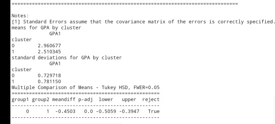
3. Results
I used eleven variables to represent the characteristics that could have some impact in the school achievement.
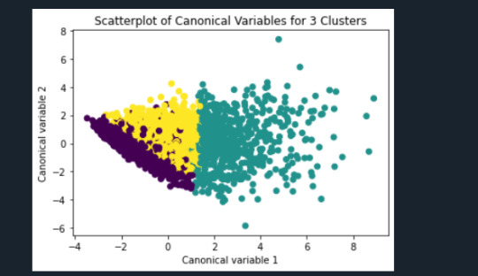
In order to visualize this vriables with K-Means clustering analysis I am using canonical variable method to reduce the eleven variables in two.
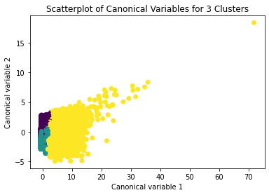
In the following image we can see the K-Means clustering result over the data:
In the previous image, we can see that the green and yellow clusters are closely packed for that we can think that the soluction with two clusters will be more efficient for this data.
FInally, the results obtaining with Python for the elevent variables and the clusters are shown:

1 note
·
View note
Text
K-Means clustering in Python
We are running K-Means algorithm to cluster groups of students according to some features that allow us to detect the school connectedness' level
Import Libraries:
from pandas import Series, DataFrame import pandas as pd import numpy as np import matplotlib.pylab as plt from sklearn.model_selection import train_test_split from sklearn import preprocessing from sklearn.cluster import KMeans
Read and clear data to drop NA values and keep only the features that we going to analize:
data = pd.read_csv("tree_addhealth.csv")
data.columns = map(str.upper, data.columns)
data_clean = data.dropna()
cluster=data_clean[['ALCEVR1','MAREVER1','ALCPROBS1','DEVIANT1','VIOL1', 'DEP1','ESTEEM1','SCHCONN1','PARACTV', 'PARPRES','FAMCONCT']] cluster.describe()
To apply clustering, we need to set the data in similar ranges
clustervar=cluster.copy() clustervar['ALCEVR1']=preprocessing.scale(clustervar['ALCEVR1'].astype('float64')) clustervar['ALCPROBS1']=preprocessing.scale(clustervar['ALCPROBS1'].astype('float64')) clustervar['MAREVER1']=preprocessing.scale(clustervar['MAREVER1'].astype('float64')) clustervar['DEP1']=preprocessing.scale(clustervar['DEP1'].astype('float64')) clustervar['ESTEEM1']=preprocessing.scale(clustervar['ESTEEM1'].astype('float64')) clustervar['VIOL1']=preprocessing.scale(clustervar['VIOL1'].astype('float64')) clustervar['DEVIANT1']=preprocessing.scale(clustervar['DEVIANT1'].astype('float64')) clustervar['FAMCONCT']=preprocessing.scale(clustervar['FAMCONCT'].astype('float64')) clustervar['SCHCONN1']=preprocessing.scale(clustervar['SCHCONN1'].astype('float64')) clustervar['PARACTV']=preprocessing.scale(clustervar['PARACTV'].astype('float64')) clustervar['PARPRES']=preprocessing.scale(clustervar['PARPRES'].astype('float64'))
clustervar
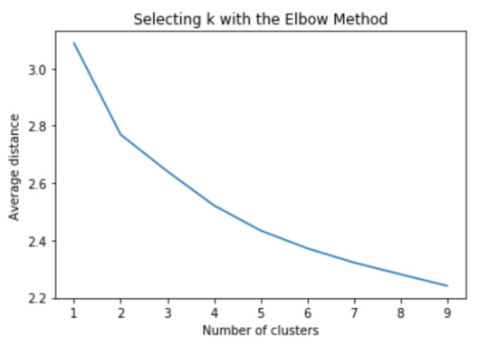
Now we can apply clustering, but before that, we need to know how many clusters would be the optimal. For that, we going to use the elbow method to graph the disantance means of each cluster
clus_train, clus_test = train_test_split(clustervar, test_size=.3, random_state=123)
from scipy.spatial.distance import cdist clusters=range(1,10) meandist=[]
for k in clusters: model=KMeans(n_clusters=k) model.fit(clus_train) clusassign=model.predict(clus_train) meandist.append(sum(np.min(cdist(clus_train, model.cluster_centers_, 'euclidean'), axis=1)) / clus_train.shape[0])
plt.plot(clusters, meandist) plt.xlabel('Number of clusters') plt.ylabel('Average distance') plt.title('Selecting k with the Elbow Method')
model3=KMeans(n_clusters=3) model3.fit(clus_train) clusassign=model3.predict(clus_train)
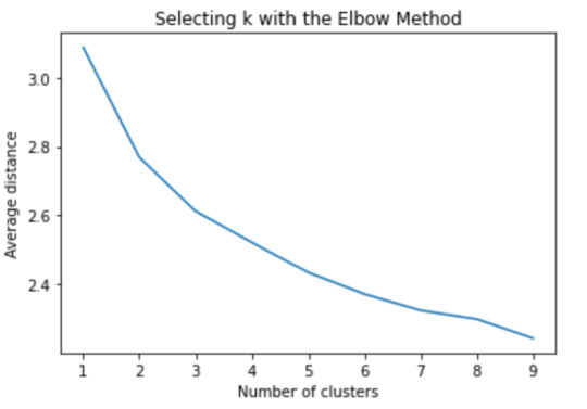
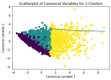
The elbow method suggest 2 or 3 clusters according to the graph
To plot the clusters, we need to reduce the variables, hence we transform the current variables into a canonical variables
from sklearn.decomposition import PCA pca_2 = PCA(2) plot_columns = pca_2.fit_transform(clus_train) plt.scatter(x=plot_columns[:,0], y=plot_columns[:,1], c=model3.labels_,) plt.xlabel('Canonical variable 1') plt.ylabel('Canonical variable 2') plt.title('Scatterplot of Canonical Variables for 3 Clusters') plt.show()
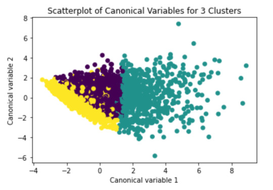
We can see a strong correlation between 2 clusters (Yellow & Purple)
Finally we group the clusters to evaluate the created model
clus_train.reset_index(level=0, inplace=True)
cluslist=list(clus_train['index'])
labels=list(model3.labels_)
newlist=dict(zip(cluslist, labels)) newlist
newclus=DataFrame.from_dict(newlist, orient='index') newclus
newclus.columns = ['cluster']
newclus.reset_index(level=0, inplace=True)
merged_train=pd.merge(clus_train, newclus, on='index') merged_train.head(n=100)
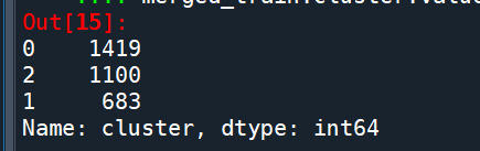
merged_train.cluster.value_counts()
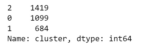
This shows the elements by cluster
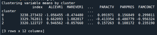
clustergrp = merged_train.groupby('cluster').mean() print ("Clustering variable means by cluster") print(clustergrp)
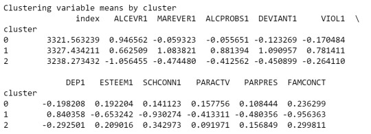
As we can see, Cluster 1 is strong in Marever 1 (use of marijuana) and Alcprobs1 (use of alcohol), on the other hand, cluster 2 is strong in Schconn (school connectedness) and Esteem1 (self esteem).
We can evaluate the relation between clusters
gpa_data=data_clean['GPA1']
gpa_train, gpa_test = train_test_split(gpa_data, test_size=.3, random_state=123) gpa_train1=pd.DataFrame(gpa_train) gpa_train1.reset_index(level=0, inplace=True) merged_train_all=pd.merge(gpa_train1, merged_train, on='index') sub1 = merged_train_all[['GPA1', 'cluster']].dropna()
import statsmodels.formula.api as smf import statsmodels.stats.multicomp as multi
gpamod = smf.ols(formula='GPA1 ~ C(cluster)', data=sub1).fit() print (gpamod.summary())
print ('means for GPA by cluster') m1= sub1.groupby('cluster').mean() print (m1)
print ('standard deviations for GPA by cluster') m2= sub1.groupby('cluster').std() print (m2)
mc1 = multi.MultiComparison(sub1['GPA1'], sub1['cluster']) res1 = mc1.tukeyhsd() print(res1.summary())

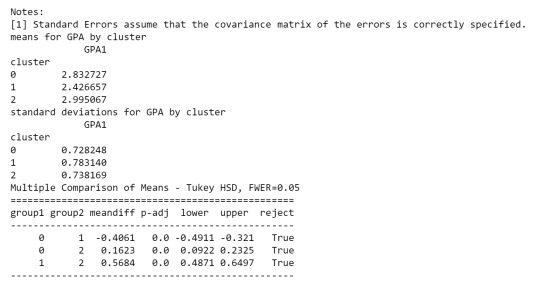
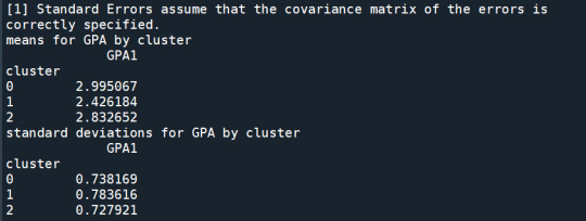
As we can see, the first table shows us data regarding the relationship between each cluster, which indicates that there is a considerable difference.
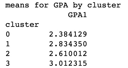
in the second table, we can see de GPA (Grade Point Average) is higher in cluster 2 where the features related to positive aspects regarding the use of alcohol and marijuana
0 notes
Text
Running a k-means Cluster Analysis
from pandas import Series, DataFrame import pandas as pd import numpy as np import os import matplotlib.pylab as plt
from sklearn.cross_validation import train_test_split
from sklearn.model_selection import train_test_split from sklearn import preprocessing from sklearn.cluster import KMeans
""" Data Management """ os.chdir("C:\TREES") data = pd.read_csv("tree_addhealth.csv")
upper-case all DataFrame column names
data.columns = map(str.upper, data.columns)
Data Management
data_clean = data.dropna()
subset clustering variables
cluster=data_clean[['ALCEVR1','MAREVER1','ALCPROBS1','DEVIANT1','VIOL1', 'DEP1','ESTEEM1','SCHCONN1','PARACTV', 'PARPRES','FAMCONCT']] cluster.describe()
standardize clustering variables to have mean=0 and sd=1
clustervar=cluster.copy() clustervar['ALCEVR1']=preprocessing.scale(clustervar['ALCEVR1'].astype('float64')) clustervar['ALCPROBS1']=preprocessing.scale(clustervar['ALCPROBS1'].astype('float64')) clustervar['MAREVER1']=preprocessing.scale(clustervar['MAREVER1'].astype('float64')) clustervar['DEP1']=preprocessing.scale(clustervar['DEP1'].astype('float64')) clustervar['ESTEEM1']=preprocessing.scale(clustervar['ESTEEM1'].astype('float64')) clustervar['VIOL1']=preprocessing.scale(clustervar['VIOL1'].astype('float64')) clustervar['DEVIANT1']=preprocessing.scale(clustervar['DEVIANT1'].astype('float64')) clustervar['FAMCONCT']=preprocessing.scale(clustervar['FAMCONCT'].astype('float64')) clustervar['SCHCONN1']=preprocessing.scale(clustervar['SCHCONN1'].astype('float64')) clustervar['PARACTV']=preprocessing.scale(clustervar['PARACTV'].astype('float64')) clustervar['PARPRES']=preprocessing.scale(clustervar['PARPRES'].astype('float64'))
split data into train and test sets
clus_train, clus_test = train_test_split(clustervar, test_size=.3, random_state=123)
k-means cluster analysis for 1-9 clusters
from scipy.spatial.distance import cdist clusters=range(1,10) meandist=[]
for k in clusters: model=KMeans(n_clusters=k) model.fit(clus_train) clusassign=model.predict(clus_train) meandist.append(sum(np.min(cdist(clus_train, model.cluster_centers_, 'euclidean'), axis=1)) / clus_train.shape[0])
""" Plot average distance from observations from the cluster centroid to use the Elbow Method to identify number of clusters to choose """
plt.plot(clusters, meandist) plt.xlabel('Number of clusters') plt.ylabel('Average distance') plt.title('Selecting k with the Elbow Method')
Interpret 3 cluster solution
model3=KMeans(n_clusters=3) model3.fit(clus_train) clusassign=model3.predict(clus_train)
plot clusters
from sklearn.decomposition import PCA pca_2 = PCA(2) plot_columns = pca_2.fit_transform(clus_train) plt.scatter(x=plot_columns[:,0], y=plot_columns[:,1], c=model3.labels_,) plt.xlabel('Canonical variable 1') plt.ylabel('Canonical variable 2') plt.title('Scatterplot of Canonical Variables for 3 Clusters') plt.show()
""" BEGIN multiple steps to merge cluster assignment with clustering variables to examine cluster variable means by cluster """
create a unique identifier variable from the index for the
cluster training data to merge with the cluster assignment variable
clus_train.reset_index(level=0, inplace=True)
create a list that has the new index variable
cluslist=list(clus_train['index'])
create a list of cluster assignments
labels=list(model3.labels_)
combine index variable list with cluster assignment list into a dictionary
newlist=dict(zip(cluslist, labels)) newlist
convert newlist dictionary to a dataframe
newclus=DataFrame.from_dict(newlist, orient='index') newclus
rename the cluster assignment column
newclus.columns = ['cluster']
now do the same for the cluster assignment variable
create a unique identifier variable from the index for the
cluster assignment dataframe
to merge with cluster training data
newclus.reset_index(level=0, inplace=True)
merge the cluster assignment dataframe with the cluster training variable dataframe
by the index variable
merged_train=pd.merge(clus_train, newclus, on='index') merged_train.head(n=100)
cluster frequencies
merged_train.cluster.value_counts()
""" END multiple steps to merge cluster assignment with clustering variables to examine cluster variable means by cluster """
FINALLY calculate clustering variable means by cluster
clustergrp = merged_train.groupby('cluster').mean() print ("Clustering variable means by cluster") print(clustergrp)
validate clusters in training data by examining cluster differences in GPA using ANOVA
first have to merge GPA with clustering variables and cluster assignment data
gpa_data=data_clean['GPA1']
split GPA data into train and test sets
gpa_train, gpa_test = train_test_split(gpa_data, test_size=.3, random_state=123) gpa_train1=pd.DataFrame(gpa_train) gpa_train1.reset_index(level=0, inplace=True) merged_train_all=pd.merge(gpa_train1, merged_train, on='index') sub1 = merged_train_all[['GPA1', 'cluster']].dropna()
import statsmodels.formula.api as smf import statsmodels.stats.multicomp as multi
gpamod = smf.ols(formula='GPA1 ~ C(cluster)', data=sub1).fit() print (gpamod.summary())
print ('means for GPA by cluster') m1= sub1.groupby('cluster').mean() print (m1)
print ('standard deviations for GPA by cluster') m2= sub1.groupby('cluster').std() print (m2)
mc1 = multi.MultiComparison(sub1['GPA1'], sub1['cluster']) res1 = mc1.tukeyhsd() print(res1.summary())
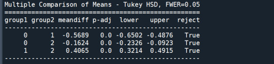
In order to externally validate the clusters, an Analysis of Variance (ANOVA) was conducting to test for significant differences between the clusters on grade point average (GPA). A tukey test was used for post hoc comparisons between the clusters. Results indicated significant differences between the clusters on GPA (F(3, 3197)=82.28, p<.0001). The tukey post hoc comparisons showed significant differences between clusters on GPA, with the exception that clusters 1 and 2 were not significantly different from each other. Adolescents in cluster 4 had the highest GPA (mean=2.99, sd=0.73), and cluster 3 had the lowest GPA (mean=2.42, sd=0.78).
0 notes
Text
Week 4 K-Cluster Analysis
from pandas import Series, DataFrame import pandas as pd import numpy as np import matplotlib.pylab as plt from sklearn.model_selection import train_test_split from sklearn import preprocessing from sklearn.cluster import KMeans import os file = open(os.path.expanduser("~/Desktop/TreeAddHealth.csv")) # Load and manage data AH_data = pd.read_csv(file) AH_data.columns = map(str.upper, AH_data.columns) data_clean = AH_data.dropna() # subset clustering variables cluster = data_clean[['ALCEVR1', 'MAREVER1', 'ALCPROBS1', 'DEVIANT1', 'VIOL1', 'DEP1', 'ESTEEM1', 'SCHCONN1', 'PARACTV', 'PARPRES', 'FAMCONCT']] cluster.describe() # standardize clustering variables to have mean=0 & sd=1 clustervar = cluster.copy() clustervar['ALCEVR1'] = preprocessing.scale(clustervar['ALCEVR1'].astype('float64')) clustervar['ALCPROBS1'] = preprocessing.scale(clustervar['ALCPROBS1'].astype('float64')) clustervar['MAREVER1'] = preprocessing.scale(clustervar['MAREVER1'].astype('float64')) clustervar['DEP1'] = preprocessing.scale(clustervar['DEP1'].astype('float64')) clustervar['ESTEEM1'] = preprocessing.scale(clustervar['ESTEEM1'].astype('float64')) clustervar['VIOL1'] = preprocessing.scale(clustervar['VIOL1'].astype('float64')) clustervar['DEVIANT1'] = preprocessing.scale(clustervar['DEVIANT1'].astype('float64')) clustervar['FAMCONCT'] = preprocessing.scale(clustervar['FAMCONCT'].astype('float64')) clustervar['SCHCONN1'] = preprocessing.scale(clustervar['SCHCONN1'].astype('float64')) clustervar['PARACTV'] = preprocessing.scale(clustervar['PARACTV'].astype('float64')) clustervar['PARPRES'] = preprocessing.scale(clustervar['PARPRES'].astype('float64')) # split data in train & test sets clus_train, clus_test, = train_test_split(clustervar, test_size=.3, random_state=123) # k-means cluster analysis for 1-9 clusters from scipy.spatial.distance import cdist clusters = range(1, 10) meandist = [] for k in clusters: model = KMeans(n_clusters=k) model.fit(clus_train) clusassign = model.predict(clus_train) meandist.append(sum(np.min(cdist(clus_train, model.cluster_centers_, 'euclidean'), axis=1))) # plt.plot(clusters, meandist) >> comment out to hide plt.xlabel('Number of clusters') plt.ylabel('Average distance') plt.title('Selecting k with the Elbow method') # Interpret 3 cluster solution model3 = KMeans(n_clusters=3) model3.fit(clus_train) clusassign = model3.predict(clus_train) # plot clusters from sklearn.decomposition import PCA pca_2 = PCA(2) plot_columns = pca_2.fit_transform(clus_train) plt.scatter(x=plot_columns[:, 0], y=plot_columns[:, 1], c=model3.labels_) plt.xlabel('Canonical variable 1') plt.ylabel('Canonical variable 2') plt.title('Scatterplot of Canonical Variables for 3 Clusters') # plt.show() # create a unique identifier variable from the index clus_train.reset_index(level=0, inplace=True) # create a list for the new index variable cluslist = list(clus_train['index']) # create a list of cluster assignments labels = list(model3.labels_) # combine index variable list with cluster assignment list into a dictionary, dataframe newlist = dict(zip(cluslist, labels)) newlist newclus = DataFrame.from_dict(newlist, orient='index') newclus newclus.columns = ['cluster'] newclus.reset_index(level=0, inplace=True) merged_train = pd.merge(clus_train, newclus, on='index') merged_train.head(n=100) # cluster frequencies merged_train.cluster.value_counts() # calculate clustering variable means by cluster clustergrp = merged_train.groupby('cluster').mean() # print("Clustering variable means by cluster") # print(clustergrp) # validate clusters in training data gpa_data = data_clean['GPA1'] # create train & test sets gpa_train, gpa_test = train_test_split(gpa_data, test_size=.3, random_state=123) gpa_train1 = pd.DataFrame(gpa_train) gpa_train1.reset_index(level=0, inplace=True) merged_train_all = pd.merge(gpa_train1, merged_train, on='index') sub1 = merged_train_all[['GPA1', 'cluster']].dropna() import statsmodels.formula.api as smf import statsmodels.stats.multicomp as multi gpamod = smf.ols(formula='GPA1 ~ C(cluster)', data=sub1).fit() print(gpamod.summary()) print('means for GPA by cluster') m1 = sub1.groupby('cluster').mean() print(m1) print('Standard deviations for GPA by cluster') m2 = sub1.groupby('cluster').std() print(m2) mc1 = multi.MultiComparison(sub1['GPA1'], sub1['cluster']) res1 = mc1.tukeyhsd() print(res1.summary)
OUTPUT:
OLS Regression Results ============================================================================== Dep. Variable: GPA1 R-squared: 0.077 Model: OLS Adj. R-squared: 0.076 Method: Least Squares F-statistic: 133.3 Date: Wed, 11 May 2022 Prob (F-statistic): 2.50e-56 Time: 18:48:25 Log-Likelihood: -3599.3 No. Observations: 3202 AIC: 7205. Df Residuals: 3199 BIC: 7223. Df Model: 2 Covariance Type: nonrobust =================================================================================== coef std err t P>|t| [0.025 0.975] ----------------------------------------------------------------------------------- Intercept 2.9945 0.020 151.472 0.000 2.956 3.033 C(cluster)[T.1] -0.5685 0.035 -16.314 0.000 -0.637 -0.500 C(cluster)[T.2] -0.1646 0.030 -5.512 0.000 -0.223 -0.106 ============================================================================== Omnibus: 154.326 Durbin-Watson: 2.019 Prob(Omnibus): 0.000 Jarque-Bera (JB): 92.624 Skew: -0.277 Prob(JB): 7.71e-21 Kurtosis: 2.377 Cond. No. 3.41 ==============================================================================
Notes: [1] Standard Errors assume that the covariance matrix of the errors is correctly specified. means for GPA by cluster GPA1 cluster 0 2.994542 1 2.426063 2 2.829949 Standard deviations for GPA by cluster GPA1 cluster 0 0.738174 1 0.786903 2 0.727230 <bound method TukeyHSDResults.summary of <statsmodels.sandbox.stats.multicomp.TukeyHSDResults object at 0x157a87520>>
Process finished with exit code 0
0 notes
Photo
Code:
data = pd.read_csv("marscrater_pds.csv")
cluster=data_clean[['LATITUDE_CIRCLE_IMAGE','LONGITUDE_CIRCLE_IMAGE', 'DIAM_CIRCLE_IMAGE', 'DEPTH_RIMFLOOR_TOPOG','NUMBER_LAYERS']] cluster.describe()
# standardize clustering variables to have mean=0 and sd=1 clustervar=cluster.copy() clustervar['LATITUDE_CIRCLE_IMAGE']=preprocessing.scale(clustervar['LATITUDE_CIRCLE_IMAGE'].astype('float64')) clustervar['LONGITUDE_CIRCLE_IMAGE']=preprocessing.scale(clustervar['LONGITUDE_CIRCLE_IMAGE'].astype('float64')) clustervar['DIAM_CIRCLE_IMAGE']=preprocessing.scale(clustervar['DIAM_CIRCLE_IMAGE'].astype('float64')) clustervar['DEPTH_RIMFLOOR_TOPOG']=preprocessing.scale(clustervar['DEPTH_RIMFLOOR_TOPOG'].astype('float64')) clustervar['NUMBER_LAYERS']=preprocessing.scale(clustervar['NUMBER_LAYERS'].astype('float64'))
# split data into train and test sets clus_train, clus_test = train_test_split(clustervar, test_size=.3, random_state=123)
# k-means cluster analysis for 1-9 clusters from scipy.spatial.distance import cdist clusters=range(1,10) meandist=[]
for k in clusters: model=KMeans(n_clusters=k) model.fit(clus_train) clusassign=model.predict(clus_train) meandist.append(sum(np.min(cdist(clus_train, model.cluster_centers_, 'euclidean'), axis=1)) / clus_train.shape[0])
plt.plot(clusters, meandist)
plt.xlabel('Number of clusters') plt.ylabel('Average distance') plt.title('Selecting k with the Elbow Method')
# Interpret 3 cluster solution model3=KMeans(n_clusters=3) model3.fit(clus_train) clusassign=model3.predict(clus_train) # plot clusters
from sklearn.decomposition import PCA pca_2 = PCA(2) plot_columns = pca_2.fit_transform(clus_train) plt.scatter(x=plot_columns[:,0], y=plot_columns[:,1], c=model3.labels_,) plt.xlabel('Canonical variable 1') plt.ylabel('Canonical variable 2') plt.title('Scatterplot of Canonical Variables for 3 Clusters') plt.show()
clus_train.reset_index(level=0, inplace=True) cluslist=list(clus_train['index']) labels=list(model3.labels_) # combine index variable list with cluster assignment list into a dictionary newlist=dict(zip(cluslist, labels)) newlist # convert newlist dictionary to a dataframe newclus=DataFrame.from_dict(newlist, orient='index') newclus # rename the cluster assignment column newclus.columns = ['cluster']
newclus.reset_index(level=0, inplace=True) merged_train=pd.merge(clus_train, newclus, on='index') merged_train.head(n=100) merged_train.cluster.value_counts()
clustergrp = merged_train.groupby('cluster').mean()
print ("Clustering variable means by cluster") print(clustergrp)
Summary: Created a K-means cluster analysis using the marscrater data provided and niticed three clusters. The tukey test shows that the clusters differed significantly in no. of layers.
0 notes
Text
K-means Clustering
My codes are as follows:
from pandas import Series, DataFrame import pandas as pd import numpy as np import matplotlib.pylab as plt from sklearn.cross_validation import train_test_split from sklearn import preprocessing from sklearn.cluster import KMeans
""" Data Management """ data = pd.read_csv("tree_addhealth.csv")
#upper-case all DataFrame column names data.columns = map(str.upper, data.columns)
# Data Management
data_clean = data.dropna()
# subset clustering variables cluster=data_clean[['ALCEVR1','MAREVER1','ALCPROBS1','DEVIANT1','VIOL1', 'DEP1','ESTEEM1','SCHCONN1','PARACTV', 'PARPRES','FAMCONCT']] cluster.describe()
# standardize clustering variables to have mean=0 and sd=1 clustervar=cluster.copy() clustervar['ALCEVR1']=preprocessing.scale(clustervar['ALCEVR1'].astype('float64')) clustervar['ALCPROBS1']=preprocessing.scale(clustervar['ALCPROBS1'].astype('float64')) clustervar['MAREVER1']=preprocessing.scale(clustervar['MAREVER1'].astype('float64')) clustervar['DEP1']=preprocessing.scale(clustervar['DEP1'].astype('float64')) clustervar['ESTEEM1']=preprocessing.scale(clustervar['ESTEEM1'].astype('float64')) clustervar['VIOL1']=preprocessing.scale(clustervar['VIOL1'].astype('float64')) clustervar['DEVIANT1']=preprocessing.scale(clustervar['DEVIANT1'].astype('float64')) clustervar['FAMCONCT']=preprocessing.scale(clustervar['FAMCONCT'].astype('float64')) clustervar['SCHCONN1']=preprocessing.scale(clustervar['SCHCONN1'].astype('float64')) clustervar['PARACTV']=preprocessing.scale(clustervar['PARACTV'].astype('float64')) clustervar['PARPRES']=preprocessing.scale(clustervar['PARPRES'].astype('float64'))
# split data into train and test sets clus_train, clus_test = train_test_split(clustervar, test_size=.3, random_state=123)
# k-means cluster analysis for 1-9 clusters from scipy.spatial.distance import cdist clusters=range(1,10) meandist=[]
for k in clusters: model=KMeans(n_clusters=k) model.fit(clus_train) clusassign=model.predict(clus_train) meandist.append(sum(np.min(cdist(clus_train, model.cluster_centers_, 'euclidean'), axis=1)) / clus_train.shape[0])
""" Plot average distance from observations from the cluster centroid to use the Elbow Method to identify number of clusters to choose """
plt.plot(clusters, meandist) plt.xlabel('Number of clusters') plt.ylabel('Average distance') plt.title('Selecting k with the Elbow Method')
# Interpret 4 cluster solution model3=KMeans(n_clusters=4) model3.fit(clus_train) clusassign=model3.predict(clus_train) # plot clusters
from sklearn.decomposition import PCA pca_2 = PCA(2) plot_columns = pca_2.fit_transform(clus_train) plt.scatter(x=plot_columns[:,0], y=plot_columns[:,1], c=model3.labels_,) plt.xlabel('Canonical variable 1') plt.ylabel('Canonical variable 2') plt.title('Scatterplot of Canonical Variables for 4 Clusters') plt.show()
""" BEGIN multiple steps to merge cluster assignment with clustering variables to examine cluster variable means by cluster """ # create a unique identifier variable from the index for the # cluster training data to merge with the cluster assignment variable clus_train.reset_index(level=0, inplace=True) # create a list that has the new index variable cluslist=list(clus_train['index']) # create a list of cluster assignments labels=list(model3.labels_) # combine index variable list with cluster assignment list into a dictionary newlist=dict(zip(cluslist, labels)) newlist # convert newlist dictionary to a dataframe newclus=DataFrame.from_dict(newlist, orient='index') newclus # rename the cluster assignment column newclus.columns = ['cluster']
# now do the same for the cluster assignment variable # create a unique identifier variable from the index for the # cluster assignment dataframe # to merge with cluster training data newclus.reset_index(level=0, inplace=True) # merge the cluster assignment dataframe with the cluster training variable dataframe # by the index variable merged_train=pd.merge(clus_train, newclus, on='index') merged_train.head(n=100) # cluster frequencies merged_train.cluster.value_counts()
""" END multiple steps to merge cluster assignment with clustering variables to examine cluster variable means by cluster """
# FINALLY calculate clustering variable means by cluster clustergrp = merged_train.groupby('cluster').mean() print ("Clustering variable means by cluster") print(clustergrp)
# validate clusters in training data by examining cluster differences in GPA using ANOVA # first have to merge GPA with clustering variables and cluster assignment data gpa_data=data_clean['GPA1'] # split GPA data into train and test sets gpa_train, gpa_test = train_test_split(gpa_data, test_size=.3, random_state=123) gpa_train1=pd.DataFrame(gpa_train) gpa_train1.reset_index(level=0, inplace=True) merged_train_all=pd.merge(gpa_train1, merged_train, on='index') sub1 = merged_train_all[['GPA1', 'cluster']].dropna()
import statsmodels.formula.api as smf import statsmodels.stats.multicomp as multi
gpamod = smf.ols(formula='GPA1 ~ C(cluster)', data=sub1).fit() print (gpamod.summary())
print ('means for GPA by cluster') m1= sub1.groupby('cluster').mean() print (m1)
print ('standard deviations for GPA by cluster') m2= sub1.groupby('cluster').std() print (m2)
mc1 = multi.MultiComparison(sub1['GPA1'], sub1['cluster']) res1 = mc1.tukeyhsd() print(res1.summary())
Summary:
A k-means cluster analysis was conducted to identify underlying subgroups of adolescents based on their similarity of responses on 11 variables that represent characteristics that could have an impact on school achievement. Clustering variables included two binary variables measuring whether or not the adolescent had ever used alcohol or marijuana, as well as quantitative variables measuring alcohol problems, a scale measuring engaging in deviant behaviors (such as vandalism, other property damage, lying, stealing, running away, driving without permission, selling drugs, and skipping school), and scales measuring violence, depression, self-esteem, parental presence, parental activities, family connectedness, and school connectedness. All clustering variables were standardized to have a mean of 0 and a standard deviation of 1.
Data were randomly split into a training set that included 70% of the observations (N=3201) and a test set that included 30% of the observations (N=1701). A series of k-means cluster analyses were conducted on the training data specifying k=1-9 clusters, using Euclidean distance. The variance in the clustering variables that was accounted for by the clusters (r-square) was plotted for each of the nine cluster solutions in an elbow curve to provide guidance for choosing the number of clusters to interpret.
Figure 1. Elbow curve of average distance values for the nine cluster solutions
The elbow curve was inconclusive, suggesting that the 2, 3 and 4-cluster solutions might be interpreted. The results below are for an interpretation of the 4-cluster solution.
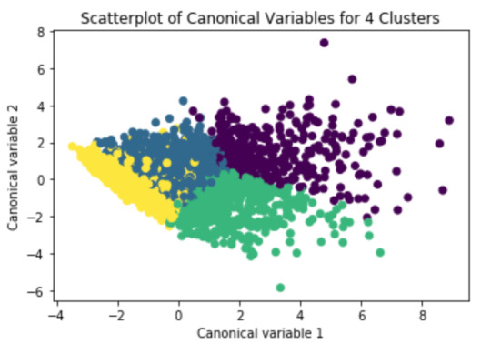
Canonical discriminant analyses was used to reduce the 11 clustering variable down a few variables that accounted for most of the variance in the clustering variables. A scatterplot of the first two canonical variables by cluster (Figure 2 shown below) indicated that the observations in 2 clusters (purple and green) were densely packed with relatively low within cluster variance, and did not overlap very much with the other clusters. Observations in the purple cluster were spread out more than the other clusters, showing high within cluster variance. But, the observations in the yellow and blue clusters overlap very much with each others. The results of this plot suggest that the best cluster solution may have fewer than 4 clusters, so it will be especially important to also evaluate the cluster solutions with fewer than 4 clusters.
Figure 2. Plot of the first two canonical variables for the clustering variables by cluster.
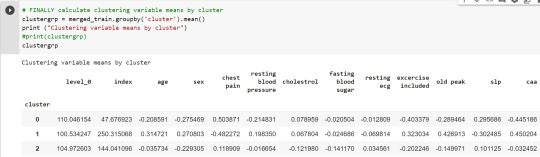
The mean values for each variables for different clusters. We could observe the differences due to the above graph.
In order to externally validate the clusters, an Analysis of Variance (ANOVA) was conducting to test for significant differences between the clusters on grade point average (GPA). Results indicated significant differences between each of the clusters. A tukey test was used for post hoc comparisons between the clusters. The tukey post hoc comparisons showed significant differences between each of all the clusters on GPA. Adolescents in cluster 3 had the highest GPA (mean=3.01), and cluster 0 had the lowest GPA (mean=2.38).
0 notes
Text
K-means Cluster Analysis for Heart attack Analysis
A k-means cluster analysis was conducted to identify underlying subgroups of individuals based on their similarity of responses on 12 variables that represent characteristics that could have an impact on maximum heart rate achieved.
Primarily, all python libraries need to be loaded that are required in creation for a lasso regression model. These also include the k-Means function from the sklearn.cluster library. Following are the libraries that are necessary to import:

Next, the required dataset is loaded. Here, I have uploaded the dataset available at Kaggle.com in the csv format using the read_csv() function. The dataset contains 14 attributes. These are age, sex, chest pain type (4 values), resting blood pressure, serum cholesterol in mg/dl, fasting blood sugar > 120 mg/dl, resting electrocardiographic results (values 0,1,2), maximum heart rate achieved, exercise induced angina, old peak = ST depression induced by exercise relative to rest, the slope of the peak exercise ST segment, number of major vessels (0-3) colored by fluoroscopy, thal: 0 = normal; 1 = fixed defect; 2 = reversible defect and output: 0= less chance of heart attack 1= more chance of heart attack.

Out of the 13 variables, only 12 were used in cluster analysis. Variable for maximum heart rate achieved is used for validation.

Before clustering, we need to standardize the variables measured on different scales. This is done so that the solution is not driven by variables measured on larger scales. The describe function is used to see statistical details of pandas dataframe. From the above data, we can see that our clustering variables are not standardized.
Here, we standardized the clustering variables to have a mean of 0, and a standard deviation of 1.The as type float 64 code ensures that all predictors will have a numeric format.
clustervar=cluster.copy()
clustervar['sex']=preprocessing.scale(clustervar['sex'].astype('float64'))
clustervar['age']=preprocessing.scale(clustervar['age'].astype('float64'))
clustervar['resting blood pressure']=preprocessing.scale(clustervar['resting blood pressure'].astype('float64'))
clustervar['cholestrol']=preprocessing.scale(clustervar['cholestrol'].astype('float64'))
clustervar['old peak']=preprocessing.scale(clustervar['old peak'].astype('float64'))
clustervar['chest pain']=preprocessing.scale(clustervar['chest pain'].astype('float64'))
clustervar['fasting blood sugar']=preprocessing.scale(clustervar['fasting blood sugar'].astype('float64'))
clustervar['resting ecg']=preprocessing.scale(clustervar['resting ecg'].astype('float64'))
clustervar['excercise included']=preprocessing.scale(clustervar['excercise included'].astype('float64'))
clustervar['slp']=preprocessing.scale(clustervar['slp'].astype('float64'))
clustervar['caa']=preprocessing.scale(clustervar['caa'].astype('float64'))
clustervar['THALL']=preprocessing.scale(clustervar['THALL'].astype('float64'))
clustervar['output']=preprocessing.scale(clustervar['output'].astype('float64'))
Now, dataset is divided into a training set and a test set. This can be achieved by using train_test_split() function. The size ratio is set as 70% for the training sample and 30% for the test sample. The random_state option specifies a random number seat(here I have selected as 123) to ensure that the data are randomly split the same way if the code is run again.
# split data into train and test sets
clus_train, clus_test = train_test_split(clustervar, test_size=.3, random_state=123)
cdist function from the scipy.spatial.distance library is used to calculate the average distance of the observations from the cluster centroids. We used 10 clusters for the analysis. Object meandist is used to store the average distance values that we will calculate for the 1 to 9 cluster solutions. The model is then initialized by calling the k-Means function from the sk learning cluster library. The function takes n_clusters which indicates the number of clusters as an argument. Here, we substituted n_clusters with k to tell Python to run the cluster analysis for 1 through 9 clusters. The model is then trained using the fit function which takes training features as argument. The code following meandist.append computes the average of the sum of the distances between each observation in the cluster centroids.
# k-means cluster analysis for 1-9 clusters
from scipy.spatial.distance import cdist
clusters=range(1,10)
meandist=[]
for k in clusters:
model=KMeans(n_clusters=k)
model.fit(clus_train)
clusassign=model.predict(clus_train)
meandist.append(sum(np.min(cdist(clus_train, model.cluster_centers_, 'euclidean'), axis=1))
/ clus_train.shape[0])
Next, we plot the elbow curve using the map plot lib plot function. The plot shows decrease in the average minimum distance of the observations from the cluster centroids for each of the cluster solutions.

From the above graph, we can see that the average distance decreases as the number of clusters increases. We can observe at two clusters, at three clusters, at seven clusters, and at eight clusters , there appear to be bends. These bends indicates that average distance value is leveling off such that adding more clusters doesn't decrease the average distance as much. Notice that these bends are not very much clear. This means that the elbow curve was inconclusive.
So we'll rerun the cluster analysis, this time asking for 3 clusters. To do so, simply initialize the model by calling the Kmeans function and set nclusters=3.
# Interpret 3 cluster solution
model3=KMeans(n_clusters=3)
model3.fit(clus_train)
clusassign=model3.predict(clus_train)
# plot clusters
Now, we used canonical discriminate analysis, which is a data reduction technique that creates a smaller number of variables that are linear combinations of the 3 clustering variables. To conduct the canonical discriminate analysis, we used the the PCA function and the sklearn decomposition library.
PCA(2) asks Python to return the two first canonical variables.Then we create a matrix called plot_columns that will include the two canonical variables estimated by the canonical discriminate analysis. PCA_2.fit asks Python to fit the canonical discriminate analysis that we specified with the PCA command, and the _transform applies the canonical discriminate analysis to the clus_train data set to calculate the canonical variables. We will plot the two canonical variables by the cluster assignment values from the 3 cluster solution in a scatter plot using the matplot libplot function.
From the above graph we can see that none of the cluster did not overlap very much with the other clusters. This indicates less correlation among the observations. The observations in the green and yellow clusters had greater spread. Also the observation in the green cluster were spread out more than the other clusters, showing high within cluster variance. The results of this plot suggest that the best cluster solution may have fewer than 3 clusters, so it will be especially important to also evaluate the cluster solutions with fewer than 3 clusters.
The means on the clustering variables showed that compared to the other clusters, individuals in cluster 0 had the highest likelihood of having a heart attack. They are less likely to get a blood disorder called thalassemia than cluster 1, highest slope of the peak exercise ST segment, lesser exercise induced angina,moderate old peak and greater chances of having a chest pain. On the other hand, indivuals in cluster 1 had the least chance of having a heart attack. Compared to individuals in the other clusters, they were lower chances for having a chest pain, greater resting blood pressure, lower resting ecg, highest exercise induced angina, highest old peak, lowest slope of the peak exercise ST segment, most number of major vessels colored by fluoroscopy, and highest chances for getting a blood disorder called thalassemia. Individuals in cluster 2 appeared to have moderate chances for having a heart attack as compared to the other two clusters. They had higher levels of resting ecg and had the least levels of old peak, least number of major vessels colored by fluoroscopy and had the lowest chances for getting thalassemia.

Finally, let's see how the clusters differ on maximum heart rate achieved. We'll use analysis of variance to test whether there are significant differences between clusters on the quantitative max_heart_rate variable. To do this, we have to import the statsmodels.formula.api and the statsmodels.stats.multicomp libraries. We use the ols function to test the analysis of variance.
# validate clusters in training data by examining cluster differences in GPA using ANOVA
# first have to merge GPA with clustering variables and cluster assignment data
mhr_data=data['max_heart_rate']
# split GPA data into train and test sets
mhr_train, mhr_test = train_test_split(mhr_data, test_size=.3, random_state=123)
mhr_train1=pd.DataFrame(mhr_train)
mhr_train1.reset_index(level=0, inplace=True)
merged_train_all=pd.merge(mhr_train1, merged_train, on='index')
sub1 = merged_train_all[['max_heart_rate', 'cluster']].dropna()
import statsmodels.formula.api as smf
import statsmodels.stats.multicomp as multi
mhrmod = smf.ols(formula='max_heart_rate ~ C(cluster)', data=sub1).fit()
print (mhrmod.summary())

The analysis of variance summary table indicates that the clusters differed significantly on maximum heart rate achieved.
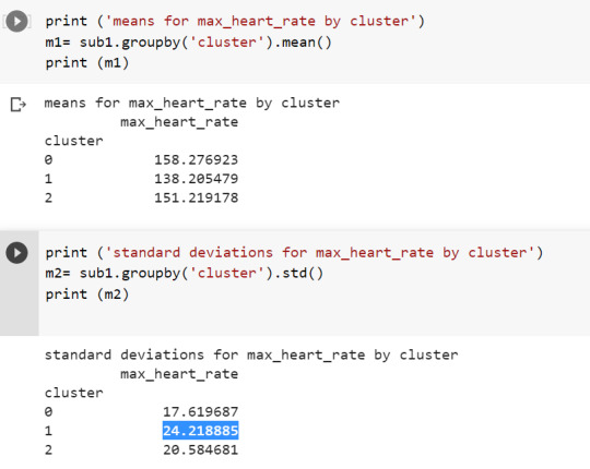
When we examine the means we find that individuals in cluster 0 had previously achieved highest heart rate(mean= 158.276923 and sd = 17.619687) and the individuals in cluster 1 had achieved the lowest levels for maximum heart rate(mean= 138.205479 and sd= 24.218885).
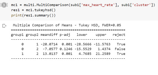
The tukey post hoc comparisons showed significant differences between clusters on maximum heart rate achieved.
0 notes
Text
K-Means Cluster Analysis
Introduction
Throughout the course I have been looking at the association of alcohol dependence and alcohol consumption in relation to multiple explanatory variables (such as alcoholic parents) using the NESARC dataset. For this assignment I will be applying a k-means cluster model to 9 selected variables to represent the characteristics of the population. I ultimately be assessing these clusters and their normal alcohol consumption, trying to understand if there is a significant difference between them.
Data Management
The below code is for importing and cleaning the data prior to modelling.
# import libraries
import pandas as pd
import numpy as np
import matplotlib.pyplot as plt
from sklearn.model_selection import train_test_split
from sklearn import preprocessing
from sklearn.cluster import KMeans
#import data
df = pd.read_csv(r'nesarc_pds.csv', low_memory=False, usecols=['S2AQ8B','S2AQ16B','S2AQ14','S1Q24FT','S1Q24IN','S1Q24LB'
,'AGE','SEX','NUMPERS','S2DQ1','S2DQ2'])
#rename columns
df.rename(columns={'S2AQ8B':'NoOfDrinks','S2AQ16B':'AgeDrinkOnceAWeek','S2AQ14':'NoYrsDrnkSame','S1Q24LB':'Weight',
'S2DQ1':'FatherAlc','S2DQ2':'MotherAlc'}, inplace=True)
# functions to calculate height
def heightInInches(feet, inches):
if (feet != 99) & (inches != 99):
return (feet * 12) + inches
else:
return np.nan
# recode values
df['FatherAlc'] = df['FatherAlc'].map({1:1, 2:0, 9:np.nan})
df['MotherAlc'] = df['MotherAlc'].map({1:1, 2:0, 9:np.nan})
df['Male'] = df['SEX'].map({1:1, 2:0})
df['Weight'].replace(999, np.nan, inplace=True)
# apply functions
df['Height'] = list(map(heightInInches, df['S1Q24FT'], df['S1Q24IN']))
# cleanse 99 and blanks
cleanse_list = ['NoOfDrinks','AgeDrinkOnceAWeek','NoYrsDrnkSame']
for col in cleanse_list:
df[col] = df[col].replace('99', np.nan)
df[col] = df[col].replace(r'^\s*$', np.nan, regex=True)
df[col] = pd.to_numeric(df[col])
cleansedData = df[['NUMPERS', 'AGE','Weight', 'NoOfDrinks','NoYrsDrnkSame', 'AgeDrinkOnceAWeek', 'FatherAlc', 'MotherAlc',
'Height', 'Male']].copy()
cleansedData.dropna(inplace=True)
cleansedData.shape
# standardise variables
variables = ['NUMPERS', 'AGE', 'Weight','NoYrsDrnkSame',
'AgeDrinkOnceAWeek', 'FatherAlc', 'MotherAlc', 'Height', 'Male']
cluster=cleansedData[variables].copy()
for col in variables:
cluster[col] = preprocessing.scale(cluster[col].astype('float64'))
# split data into train and test
clus_train, clus_test = train_test_split(cluster, test_size=.3, random_state=123)
Cluster Model
# creating a cluster analysis for 1 -9 clusters
from scipy.spatial.distance import cdist
clusters=range(1,10)
mean_dist=[]
# iterate over 1 -9 clusters to assess suitable number
for k in clusters:
model=KMeans(n_clusters=k)
model.fit(clus_train)
clus_assign=model.predict(clus_train)
mean_dist.append(sum(np.min(cdist(clus_train, model.cluster_centers_, 'euclidean'), axis=1))
/ clus_train.shape[0])
# plot the average distance from the observations from the cluster centroids
plt.plot(clusters, mean_dist)
plt.xlabel('Number of Clusters')
plt.ylabel('average distance')
plt.title('Selectingk with the Elbow Method')

# looking at 2 clusters, where the model starts to level off
model2=KMeans(n_clusters=2)
model2.fit(clus_train)
clusassign=model2.predict(clus_train)
Canonical Discriminant Analysis
# use PCA - canonical discirminant analysis as reduction technique
from sklearn.decomposition import PCA
pca_2 = PCA(2)
plot_columns = pca_2.fit_transform(clus_train)
plt.scatter(x=plot_columns[:,0], y=plot_columns[:,1], c=model2.labels_,)
plt.xlabel('Canonical Variable 1')
plt.ylabel('Canonical Variable 2')
plt.title('Scatterplot of Canonical Variables for 2 clusters')
plt.show()

Cluster metrics & ANOVA
# understanding the clusters
clus_train.reset_index(level=0, inplace=True)
cluslist=list(clus_train['index'])
labels=list(model2.labels_)
newlist=dict(zip(cluslist, labels))
newclus=pd.DataFrame.from_dict(newlist, orient='index')
newclus.columns = ['cluster']
newclus.reset_index(level=0, inplace=True)
merged_train=pd.merge(clus_train, newclus, on='index')
merged_train.cluster.value_counts()
clustergrp = merged_train.groupby('cluster').mean()
print(clustergrp)

# comparing the number of drinks an individual usually drinks between the two groups
NoOfDrinksData = cleansedData['NoOfDrinks']
drnks_train, drnks_test = train_test_split(NoOfDrinksData, test_size=.3, random_state=123)
drnks_train1=pd.DataFrame(drnks_train)
drnks_train1.reset_index(level=0, inplace=True)
merged_train_all=pd.merge(drnks_train1, merged_train, on='index')
sub1 = merged_train_all[['NoOfDrinks','cluster']].dropna()
import statsmodels.formula.api as smf
import statsmodels.stats.multicomp as multi
drnksmod = smf.ols(formula='NoOfDrinks ~ C(cluster)', data=sub1).fit()
print(drnksmod.summary())

print('Avg No of Drinks by cluster')
print(sub1.groupby('cluster')['NoOfDrinks'].mean())
print('\n Std Dev No of Drinks by cluster')
print(sub1.groupby('cluster')['NoOfDrinks'].std())

Summary
A k-means cluster model was applied to the NESARC dataset for those that consume alcohol and returned all valid responses to the 10 variables. The 9 variables that were used for the model contained 3 binary variables (Father Alcoholic, Mother Alcoholic and Male) and 6 quantitative variables (Number of persons in household, Age, Weight, Height, Number of years drinking the same as currently do and Age drinking Once a week).
As the optimum number of clusters was unknown, the model was applied using clusters 1 – 9 to understand the most effective model. A plot was produced (as shown in the ‘Cluster Model’ section, titled: 'Selectingk with the Elbow Method'), detailing the number of clusters and the average distance – using the elbow method to determine when the average distance was levelling off, I subjectively selected points 2 and 6 for the number of clusters. Further analysis was conducted on the 2-cluster model.
Canonical discriminant analysis was applied to the 2-cluster model to reduce the number of variables to 2 in which the variables account for the variance in the original 9 variables. The 2 clusters (see scatter plot above in Canonical Discriminant Analysis section) take distinct sides however there is a considerable amount of overlap meaning there is no good separation between the clusters. The clusters are not completely dense, resulting in the variance being higher and less correlated with each other.
From the means of the cluster variables, I was able to determine the following for the 2 groups:
- Cluster 0:
o Predominately Female.
o More likely than cluster 1 to have an alcoholic parent.
o More likely than cluster 1 to start drinking at least once a week at an earlier age.
- Cluster 1:
o Predominately Male.
o Have been drinking current alcohol consumption for a longer period than cluster 0.
o Tend to be living with less people than cluster 0.
To assess the 2 clusters in association with alcohol consumption, an Analysis of Variance model was applied to determine if the was a significant difference between the two groups and the number of alcoholic drinks an individual normally consumes when drinking. Those in cluster 0 had a mean number of drinks consumed as 2.0 with a standard deviation of 1.7. Those in cluster 1 had a mean number of drinks consumed as 3.1 with a standard deviation of 2.8. The F-statistic was 758.0 with a p-value of <0.001 suggesting the two groups were significantly different in relation to alcohol consumption.
0 notes
Text
Investigating Suicide rate - Week 4
Link to Jupyter Notebook:
https://colab.research.google.com/drive/1Syor16A4F5CAU8U01eo07UxYG1zv5xDn?usp=sharing
0) Python Code
# -*- coding: utf-8 -*- """DM-Gapminder-4.ipynb
Original file is located at https://colab.research.google.com/drive/1Syor16A4F5CAU8U01eo07UxYG1zv5xDn
# Data Management Capstone Project ## A look into Suicide ### Gapminder Dataset ### Joao Paulo Rebucci Lirani ### June/21 - Week 4
### Research question: ### Is suicide rate related to employment rate or alcohol consumption in Africa, Asia and Europe?
## Imports """
import pandas as pd
import numpy as np import matplotlib.pyplot as plt import seaborn as sns from gapminder import gapminder
"""## Load Dataset"""
data=pd.read_csv('gapminder.csv',low_memory=False)
# add additional feature Region from original Gapminder dataset gapminder.country.nunique()
continent=gapminder[['country','continent']] continent.drop_duplicates(subset='country',inplace=True) continent.shape
data=pd.merge(data,continent,how='left',on='country')
"""## Basic Description of dataset"""
data.shape
print(f' The dataset has {data.shape[0]} rows (observations) and {data.shape[1]} columns (features).')
# A look at the first rows of the dataset data.head()
"""## Chosen Topics"""
# Chosen Topics # For this study, we will investigate the influence of employement and alcohol comsumption in suicide rates topic=data.copy()[['country','continent','employrate','alcconsumption','suicideper100th']] #'incomeperperson',
topic.head()
"""## Data Quality"""
topic.info()
"""## Treating missing data"""
topic.isna().sum()
# Treat empty string values '' and ' ' topic.employrate.replace({'':np.nan,' ':np.nan},inplace=True) topic.alcconsumption.replace({'':np.nan,' ':np.nan},inplace=True) topic.suicideper100th.replace({'':np.nan,' ':np.nan},inplace=True)
# Transforming variables to numeric (quantitative) topic.employrate=pd.to_numeric(topic.employrate) topic.suicideper100th=pd.to_numeric(topic.suicideper100th) topic.alcconsumption=pd.to_numeric(topic.alcconsumption)
# Drop all observations where our target variable is missing. topic.dropna(subset=['alcconsumption'],inplace=True) print(f' The dataset has {topic.shape[0]} rows (observations) and {topic.shape[1]} columns (features).')
"""### Select Rows - Continents of interest"""
# We will select Europe, Asia and Africa as our continents of interest study=topic.query(' continent =="Europe" or continent =="Asia" or continent =="Africa"') print(f' Our study dataset has {study.shape[0]} rows (observations) and {study.shape[1]} columns (features).')
study.isna().sum()
study.dropna(inplace=True)
print(f' Our study dataset has {study.shape[0]} rows (observations) and {study.shape[1]} columns (features).')
"""## Exploratory Data Analysis"""
study.describe()
"""### Univariate Analysis
#### Employment rate """
# Shape study.employrate.hist(bins=20) plt.title('Distribution of Employment rate') plt.show();
# Center print('For Employment rate:') print(f'Mode is : {study.employrate.mode()[0]}') print(f'Mean is : {study.employrate.mean()}') print(f'Median is : {study.employrate.median()}') print()
# Spread print(f'Standard deviation (SD) is : {study.employrate.std()}')
"""#### Alcohol comsumption"""
study.alcconsumption.hist(bins=20) plt.title('Distribution of Alcohol consumption') plt.show();
# Center print('For Alcohol consumption:') print(f'Mode is : {study.alcconsumption.mode()[0]}') print(f'Mean is : {study.alcconsumption.mean()}') print(f'Median is : {study.alcconsumption.median()}') print()
"""#### Target variable"""
study.suicideper100th.hist() plt.title('Distribution of Suicide rate per 100k') plt.show();
# Center print('For Suicide rate:') print(f'Mode is : {study.suicideper100th.mode()[0]}') print(f'Mean is : {study.suicideper100th.mean()}') print(f'Median is : {study.suicideper100th.median()}') print()
print('Count of Countries per continent') study.continent.value_counts(sort=False)
print('Percentage of Countries per continent') study.continent.value_counts(sort=False,normalize=True)
sns.countplot(data=study,x='continent') plt.title('Number of countries per Continent');
# Top 5 countries with the highest suicide rates study.sort_values(by='suicideper100th',ascending=False).head(5)
# Top 5 countries with the lowest suicide rates study.sort_values(by='suicideper100th',ascending=True).head(5)
"""## Creating new variables and binning numeric variables"""
emplabels=['Low','Mid-Low','Mid-High','High'] study['employRateBin']= pd.qcut(study.employrate,4,labels=emplabels)
alclabels=['Low','Mid','High'] study['alcBin']= pd.cut(study.alcconsumption,[-1,2.5,10,20],labels=alclabels)
"""### Frequency tables for variables
#### Employment rate """
study.employRateBin.value_counts(sort=False)
study.employRateBin.value_counts(sort=False,normalize=True)
study.employRateBin.value_counts(sort=False).plot(kind='bar',title='Employment rate');
"""#### Alcohol consumption"""
study.alcBin.value_counts(sort=False)
study.alcBin.value_counts(sort=False,normalize=True)
study.alcBin.value_counts(sort=False).plot(kind='bar',title='Alcohol consumption');
"""## Bivariate Analysis
### Employment rate """
sns.lmplot(data=study,x='employrate',y='suicideper100th') plt.title('Suicide rate per Employment rate');
study.employrate.corr(study.suicideper100th)
sns.barplot(data=study,x='employRateBin',y='suicideper100th') plt.title('Suicide rate per Employment rate quartiles');
"""### Alcohol Consumption"""
sns.lmplot(data=study,x='alcconsumption',y='suicideper100th') plt.title('Suicide rate per Alcohol consumption');
study.alcconsumption.corr(study.suicideper100th)
sns.barplot(data=study,x='alcBin',y='suicideper100th') plt.title('Suicide rate per Alcohol Consumption (3 bins)');
"""### All variables put together"""
pd.crosstab(study.employRateBin, study.alcBin,study.suicideper100th,aggfunc='mean',rownames=['Employment rate'],colnames=['Alcohol Consump.'])
sns.heatmap(pd.crosstab(study.employRateBin, study.alcBin,study.suicideper100th,aggfunc='mean',rownames=['Employment rate'],colnames=['Alcohol Consumption']));
1) Univariate Analysis
1.1) Employment Rate
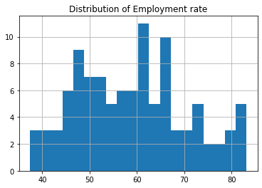
Mode is : 47.29
Mean is : 59.11
Median is : 59.19
Standard deviation (SD) is : 11.5
As we may observe, distribution of Employment rate is mainly unimodal, symmetrical (mean ~ median), centred in 60% of the population.
1.2) Alcohol consumption
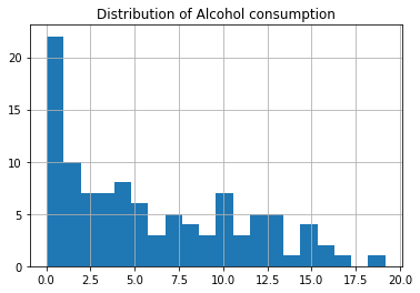
Mode is : 0.1
Mean is : 5.89
Median is : 4.42
Standard deviation (SD) is : 5.0
The distribution of Alcohol consumption is asymmetric, skewed right and mainly unimodal with a large concentration of samples in the lowest range (bin) from 0 to 1 litres per adult - the mean is 5.89 litres per adult.
1.3) Suicide rate
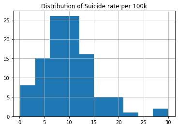
Mode is : 0.20
Mean is : 9.99
Median is : 9.23
Standard deviation (SD) is : 5.3
Our target variable, Suicide rate, has a slightly skewed-right distribution, the median is slightly below the mean, it is unimodal with its peak close to 10 suicides per 100k people.
2) Multi-variate Analysis
2.1) Employment rate and Suicide rate

Pearson Correlation coefficient: 0.13
From the scatter plot, we can observe that Suicide rate is poorly related with Employment rate - the Pearson correlation of 0.13 also indicates a very weak association between the 2 variables.
2.2) Alcohol Consumption and Suicide rate

Pearson Correlation coefficient: 0.30
From the scatter plot we may observe a weak relation between Alcohol consumption and Suicide rate - the Pearson coefficient also suggests a weak, but present, positive correlation between the two variables (stronger than previous variable) - that is , the greater the alcohol consumption, we may observe larger rates of Suicide.
Grouping alcohol consumptions into bins , it is possible to observe further:
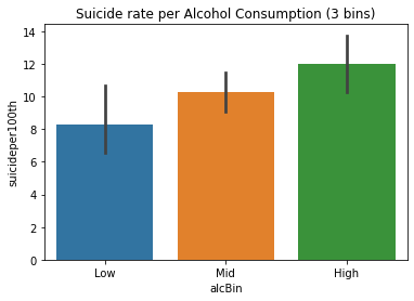
We may observe clearly that Suicide rate increases with increasing levels of Alcohol consumption.
0 notes
Text
Running a k-means Cluster Analysis
from google.colab import drive
drive.mount('/content/drive')
#import the librariesimport pandas as pd
import numpy as np
import osimport matplotlib.pyplot as plt
from sklearn.model_selection import train_test_split
from pandas import Series,DataFrame
from sklearn.cluster import KMeans
from sklearn import preprocessing
#change directory
os.chdir('/content/drive/MyDrive/MachineLearning/K_mean clustring')
#import csv_data from drive
data=pd.read_csv('tree_addhealth.csv')
#upper case from all dataframe columns name
data.columns=map(str.upper,data.columns)
#clean oservation miss data
data_clean=data.dropna()
#create clustring var
cluster=data_clean[['ALCEVR1','MAREVER1','ALCPROBS1','DEVIANT1',
'VIOL1','DEP1','ESTEEM1','SCHCONN1','PARACTV','PARPRES','FAMCONCT']]
cluster.describe()
#standerlized clusring var for maen 0 and std 1
clustervar=cluster.copy() clustervar['ALCEVR1']=preprocessing.scale(clustervar['ALCEVR1']
.astype('float64')) clustervar['ALCPROBS1']=preprocessing.scale(clustervar['ALCPROBS1']
.astype('float64')) clustervar['MAREVER1']=preprocessing.scale(clustervar['MAREVER1']
.astype('float64')) clustervar['DEP1']=preprocessing.scale(clustervar['DEP1'].astype('float64')) clustervar['ESTEEM1']=preprocessing.scale(clustervar['ESTEEM1']
.astype('float64')) clustervar['VIOL1']=preprocessing.scale(clustervar['VIOL1'].astype('float64')) clustervar['DEVIANT1']=preprocessing.scale(clustervar['DEVIANT1']
.astype('float64')) clustervar['FAMCONCT']=preprocessing.scale(clustervar['FAMCONCT']
.astype('float64')) clustervar['SCHCONN1']=preprocessing.scale(clustervar['SCHCONN1']
.astype('float64')) clustervar['PARACTV']=preprocessing.scale(clustervar['PARACTV']
.astype('float64')) clustervar['PARPRES']=preprocessing.scale(clustervar['PARPRES']
.astype('float64'))
#split data to train_set and test_set
clust_train , clust_test= train_test_split(clustervar,test_size=.3,random_state=123)
# K_mean for 1-9 analysis
from scipy.spatial.distance import cdist clusters=range(1,10) meandist=[]
for k in clusters: model=KMeans(n_clusters=k) model.fit(clus_train) clusassign=model.predict(clus_train) meandist.append(sum(np.min(cdist(clus_train, model.cluster_centers_, 'euclidean'), axis=1)) / clus_train.shape[0])
""" Plot average distance from observations from the cluster centroid to use the Elbow Method to identify number of clusters to choose """
plt.plot(clusters, meandist) plt.xlabel('Number of clusters') plt.ylabel('Average distance') plt.title('Selecting k with the Elbow Method')
# Interpret 3 cluster solution model3=KMeans(n_clusters=3) model3.fit(clus_train) clusassign=model3.predict(clus_train) # plot clusters
from sklearn.decomposition import PCA pca_2 = PCA(2) plot_columns = pca_2.fit_transform(clus_train) plt.scatter(x=plot_columns[:,0], y=plot_columns[:,1], c=model3.labels_,) plt.xlabel('Canonical variable 1') plt.ylabel('Canonical variable 2') plt.title('Scatterplot of Canonical Variables for 3 Clusters') plt.show()
""" BEGIN multiple steps to merge cluster assignment with clustering variables to examine cluster variable means by cluster """ # create a unique identifier variable from the index for the # cluster training data to merge with the cluster assignment variable clus_train.reset_index(level=0, inplace=True) # create a list that has the new index variable cluslist=list(clus_train['index']) # create a list of cluster assignments labels=list(model3.labels_) # combine index variable list with cluster assignment list into a dictionary newlist=dict(zip(cluslist, labels)) newlist # convert newlist dictionary to a dataframe newclus=DataFrame.from_dict(newlist, orient='index') newclus # rename the cluster assignment column newclus.columns = ['cluster']
# now do the same for the cluster assignment variable # create a unique identifier variable from the index for the # cluster assignment dataframe # to merge with cluster training data newclus.reset_index(level=0, inplace=True) # merge the cluster assignment dataframe with the cluster training variable dataframe # by the index variable merged_train=pd.merge(clus_train, newclus, on='index') merged_train.head(n=100) # cluster frequencies merged_train.cluster.value_counts()
""" END multiple steps to merge cluster assignment with clustering variables to examine cluster variable means by cluster """
# FINALLY calculate clustering variable means by cluster clustergrp = merged_train.groupby('cluster').mean() print ("Clustering variable means by cluster") print(clustergrp)
# validate clusters in training data by examining cluster differences in GPA using ANOVA # first have to merge GPA with clustering variables and cluster assignment data gpa_data=data_clean['GPA1'] # split GPA data into train and test sets gpa_train, gpa_test = train_test_split(gpa_data, test_size=.3, random_state=123) gpa_train1=pd.DataFrame(gpa_train) gpa_train1.reset_index(level=0, inplace=True) merged_train_all=pd.merge(gpa_train1, merged_train, on='index') sub1 = merged_train_all[['GPA1', 'cluster']].dropna()
import statsmodels.formula.api as smf import statsmodels.stats.multicomp as multi
gpamod = smf.ols(formula='GPA1 ~ C(cluster)', data=sub1).fit() print (gpamod.summary())
print ('means for GPA by cluster') m1= sub1.groupby('cluster').mean() print (m1)
print ('standard deviations for GPA by cluster') m2= sub1.groupby('cluster').std() print (m2)
mc1 = multi.MultiComparison(sub1['GPA1'], sub1['cluster']) res1 = mc1.tukeyhsd() print(res1.summary())
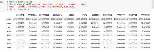

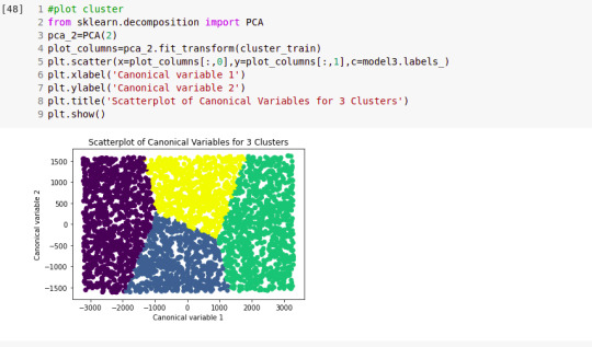
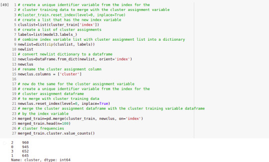
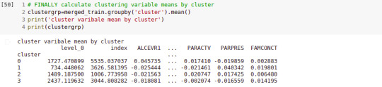
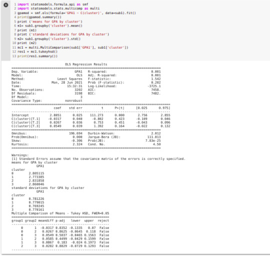
0 notes
Text
K-means clustering analysis
# standardize clustering variables to have mean=0 and sd=1 clustervar=cluster_data.copy() clustervar['ALCOHOL']=preprocessing.scale(clustervar['ALCOHOL'].astype('float64')) clustervar['MALIC_ACID']=preprocessing.scale(clustervar['MALIC_ACID'].astype('float64')) clustervar['ASH']=preprocessing.scale(clustervar['ASH'].astype('float64')) clustervar['ASH_ALCANITY']=preprocessing.scale(clustervar['ASH_ALCANITY'].astype('float64')) clustervar['MAGNESIUM']=preprocessing.scale(clustervar['MAGNESIUM'].astype('float64')) clustervar['TOTAL_PHENOLS']=preprocessing.scale(clustervar['TOTAL_PHENOLS'].astype('float64')) clustervar['FLAVANOIDS']=preprocessing.scale(clustervar['FLAVANOIDS'].astype('float64')) clustervar['NONFLAVANOID_PHENOLS']=preprocessing.scale(clustervar['NONFLAVANOID_PHENOLS'].astype('float64')) clustervar['PROANTHOCYANINS']=preprocessing.scale(clustervar['PROANTHOCYANINS'].astype('float64')) clustervar['COLOR_INTENSITY']=preprocessing.scale(clustervar['COLOR_INTENSITY'].astype('float64')) clustervar['HUE']=preprocessing.scale(clustervar['HUE'].astype('float64')) clustervar['PROLINE']=preprocessing.scale(clustervar['PROLINE'].astype('float64'))from pandas import Series, DataFrame import pandas as pd import numpy as np import os import matplotlib.pylab as plt from sklearn.model_selection import train_test_split from sklearn import preprocessing from sklearn.cluster import KMeans import sklearn.metricsIn this experimental analysis wine dataset were used to apply a K-means clustering analysis. The analysis was performed in order to identify the subgroups of wines based on the similarity of values from 12 variables. Clustering variables were included to identify the types of wines from the all observation variables, and quantitative variables such as Alcohol, Malic-acid, Ash, Alkalinity of ash, Magnesium, Total-phenols, Flavonoids, Non-flavonoid-phenols, Proanthocyanins, Color-intensity, Hue, Proline was included with clustering variables with standardized to have a mean of 0 and a standard deviation of 1.
The dataset was split into a training set that encompasses 70% of the observations(N=124) and a test set that included 30% of the observations (N=55).
Data were randomly split into a training set that included 70% of the observations (N=3201) and a test set that included 30% of the observations (N=1701). A series of k-means cluster analyses were conducted on the training data specifying k=1-9 clusters, using Euclidean distance. The variance in the clustering variables that was accounted for by the clusters (r-square) was plotted for each of the nine cluster solutions in an elbow curve to provide guidance for choosing the number of clusters to interpret.
Figure 1 Elbow curve of r-square values for the nine cluster solutions

Canonical discriminant analyses were used to reduce the 12-clustering variable down a few variables that used for the most of the variance in the clustering variables
Figure 2 Plot of the first two canonical variables for the clustering variables by cluster

======= ====The following is the python code===================
from pandas import Series, DataFrame import pandas as pd import numpy as np import os import matplotlib.pylab as plt from sklearn.model_selection import train_test_split from sklearn import preprocessing from sklearn.cluster import KMeans import sklearn.metrics
#Data Management os.chdir("E:\Python-works\dataset")
data = pd.read_csv('./wine-clustering.csv')
#upper-case all DataFrame column names data.columns = map(str.upper, data.columns)
# Data Management
data_clean = data.dropna()
# subset clustering variables cluster_data=data_clean[['ALCOHOL','MALIC_ACID','ASH','ASH_ALCANITY','MAGNESIUM', 'TOTAL_PHENOLS','FLAVANOIDS','NONFLAVANOID_PHENOLS','PROANTHOCYANINS', 'COLOR_INTENSITY','HUE','PROLINE']] cluster_data.describe()
# standardize clustering variables to have mean=0 and sd=1 clustervar=cluster_data.copy() clustervar['ALCOHOL']=preprocessing.scale(clustervar['ALCOHOL'].astype('float64')) clustervar['MALIC_ACID']=preprocessing.scale(clustervar['MALIC_ACID'].astype('float64')) clustervar['ASH']=preprocessing.scale(clustervar['ASH'].astype('float64')) clustervar['ASH_ALCANITY']=preprocessing.scale(clustervar['ASH_ALCANITY'].astype('float64')) clustervar['MAGNESIUM']=preprocessing.scale(clustervar['MAGNESIUM'].astype('float64')) clustervar['TOTAL_PHENOLS']=preprocessing.scale(clustervar['TOTAL_PHENOLS'].astype('float64')) clustervar['FLAVANOIDS']=preprocessing.scale(clustervar['FLAVANOIDS'].astype('float64')) clustervar['NONFLAVANOID_PHENOLS']=preprocessing.scale(clustervar['NONFLAVANOID_PHENOLS'].astype('float64')) clustervar['PROANTHOCYANINS']=preprocessing.scale(clustervar['PROANTHOCYANINS'].astype('float64')) clustervar['COLOR_INTENSITY']=preprocessing.scale(clustervar['COLOR_INTENSITY'].astype('float64')) clustervar['HUE']=preprocessing.scale(clustervar['HUE'].astype('float64')) clustervar['PROLINE']=preprocessing.scale(clustervar['PROLINE'].astype('float64'))
# split data into train and test sets clus_train, clus_test = train_test_split(clustervar, test_size=.3, random_state=123)
# k-means cluster analysis for 1-9 clusters from scipy.spatial.distance import cdist clusters=range(1,10) meandist=[]
for k in clusters: model=KMeans(n_clusters=k) model.fit(clus_train) clusassign=model.predict(clus_train) meandist.append(sum(np.min(cdist(clus_train, model.cluster_centers_, 'euclidean'), axis=1)) / clus_train.shape[0])
#Plot average distance from observations from the cluster centroid #to use the Elbow Method to identify number of clusters to choose plt.plot(clusters, meandist) plt.xlabel('Number of clusters') plt.ylabel('Average distance') plt.title('Selecting k with the Elbow Method')
# Interpret 3 cluster solution model3=KMeans(n_clusters=3) model3.fit(clus_train) clusassign=model3.predict(clus_train)
# plot clusters
from sklearn.decomposition import PCA pca_2 = PCA(2) plot_columns = pca_2.fit_transform(clus_train) plt.scatter(x=plot_columns[:,0], y=plot_columns[:,1], c=model3.labels_,) plt.xlabel('Canonical variable 1') plt.ylabel('Canonical variable 2') plt.title('Scatterplot of Canonical Variables for 3 Clusters') plt.show()
# create a unique identifier variable from the index for the # cluster training data to merge with the cluster assignment variable
clus_train.reset_index(level=0, inplace=True)
# create a list that has the new index variable cluslist=list(clus_train['index'])
# create a list of cluster assignments labels=list(model3.labels_)
# combine index variable list with cluster assignment list into a dictionary newlist=dict(zip(cluslist, labels)) newlist
# convert newlist dictionary to a dataframe newclus=DataFrame.from_dict(newlist, orient='index') newclus
# rename the cluster assignment column newclus.columns = ['cluster']
# now do the same for the cluster assignment variable # create a unique identifier variable from the index for the # cluster assignment dataframe # to merge with cluster training data newclus.reset_index(level=0, inplace=True)
# merge the cluster assignment dataframe with the cluster training variable dataframe # by the index variable merged_train=pd.merge(clus_train, newclus, on='index') merged_train.head(n=100)
# cluster frequencies merged_train.cluster.value_counts()
# validate clusters in training data by examining cluster differences in ODR using ANOVA # first have to merge GPA with clustering variables and cluster assignment data gpa_data=data_clean['ODR']
# split GPA data into train and test sets gpa_train, gpa_test = train_test_split(gpa_data, test_size=.3, random_state=123) gpa_train1=pd.DataFrame(gpa_train) gpa_train1.reset_index(level=0, inplace=True) merged_train_all=pd.merge(gpa_train1, merged_train, on='index') sub1 = merged_train_all[['ODR', 'cluster']].dropna()
import statsmodels.formula.api as smf import statsmodels.stats.multicomp as multi
gpamod = smf.ols(formula='ODR ~ C(cluster)', data=sub1).fit() print (gpamod.summary())
print ('means for ODR by cluster') m1= sub1.groupby('cluster').mean() print (m1)
print ('standard deviations for ODR by cluster') m2= sub1.groupby('cluster').std() print (m2)
mc1 = multi.MultiComparison(sub1['ODR'], sub1['cluster']) res1 = mc1.tukeyhsd() print(res1.summary())
#Canonical discriminant analyses were used to reduce the 12-clustering variable down a few variables that used for the most of the variance i#Figure 2 Plot of the first two canonical variables for the clustering variables by cluster
0 notes