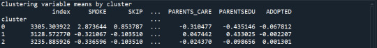
#Figure 2 Plot of the first two canonical variables for the clustering variables by cluster | Explore Tumblr posts and blogs

ggype123 · 1 year ago

Text

K-Means Cluster Analysis for Identifying Adolescent Subgroups

Introduction

A k-means cluster analysis was conducted to identify distinct subgroups of adolescents based on their responses to 11 variables associated with characteristics that could impact school achievement. The goal was to group adolescents into clusters with similar patterns of responses, providing insights into underlying subgroups.

Methodology

The analysis used the following 11 standardized clustering variables:

Binary Variables: Ever used alcohol, Ever used marijuana

Quantitative Variables:

Alcohol problems

Deviant behavior (vandalism, lying, stealing, etc.)

Violence

Depression

Self-esteem

Parental presence

Parental activities

Family connectedness

School connectedness

All variables were standardized to a mean of zero and a standard deviation of one.

The dataset was split into a training set (70% of observations, N=3201N = 3201N=3201) and a test set (30% of observations, N=1701N = 1701N=1701). K-means cluster analyses were performed on the training set for k=1k = 1k=1 to k=9k = 9k=9 clusters, using Euclidean distance. The proportion of variance accounted for by the clusters (R-squared) was plotted for each cluster solution to help determine the optimal number of clusters.

Results

Figure 1. Elbow Curve of R-Squared Values for Different Cluster Solutions

The elbow curve suggested that 2, 4, and 8-cluster solutions were plausible. The 4-cluster solution was chosen for interpretation due to its balance between complexity and interpretability.

To further explore the clusters, a canonical discriminant analysis reduced the clustering variables to two canonical variables.

Figure 2. Scatterplot of the First Two Canonical Variables by Cluster

The scatterplot showed distinct clusters with varying densities and spreads. Clusters 1 and 4 were densely packed with low within-cluster variance, while Cluster 3 showed the highest within-cluster variance.

Cluster Profiles:

Cluster 1: Adolescents with moderate levels on most variables. They had low likelihoods of using alcohol or marijuana, moderate levels of depression, and self-esteem, but relatively low school connectedness, parental presence, parental involvement, and family connectedness.

Cluster 2: Higher levels of the clustering variables compared to Cluster 1, with a higher likelihood of alcohol and marijuana use. They had moderate values compared to Clusters 3 and 4.

Cluster 3: The most troubled group. They had the highest likelihood of using alcohol and marijuana, more alcohol problems, and higher engagement in deviant and violent behaviors. They also exhibited higher depression, lower self-esteem, and the lowest levels of school connectedness, parental presence, parental involvement, and family connectedness.

Cluster 4: The least troubled group. They had the lowest likelihood of using alcohol and marijuana, the fewest alcohol problems, and the lowest engagement in deviant and violent behaviors. They also exhibited the lowest levels of depression, and higher self-esteem, school connectedness, parental presence, parental involvement, and family connectedness.

External Validation:

To validate the clusters, an Analysis of Variance (ANOVA) tested the differences in GPA between the clusters, followed by Tukey's post hoc test.

Results indicated significant differences in GPA across clusters F(3,3197)=82.28,p<.0001F(3, 3197) = 82.28, p < .0001F(3,3197)=82.28,p<.0001. Post hoc comparisons showed significant differences between all clusters except between Clusters 1 and 2.

Cluster 4: Highest GPA (mean = 2.99, SD = 0.71)

Cluster 3: Lowest GPA (mean = 2.36, SD = 0.78)

Syntax and Output

Below is the Python code used to perform the k-means clustering and the resulting output:

python

Copy code

# Import necessary libraries from sklearn.cluster import KMeans from sklearn.preprocessing import StandardScaler from sklearn.decomposition import PCA import pandas as pd import matplotlib.pyplot as plt import seaborn as sns # Load the data # Assume data is in a DataFrame 'df' X = df[['ever_used_alcohol', 'ever_used_marijuana', 'alcohol_problems', 'deviant_behavior', 'violence', 'depression', 'self_esteem', 'parental_presence', 'parental_activities', 'family_connectedness', 'school_connectedness']] # Standardize the data scaler = StandardScaler() X_scaled = scaler.fit_transform(X) # Determine the optimal number of clusters using the elbow method inertia = [] for k in range(1, 10): kmeans = KMeans(n_clusters=k, random_state=42) kmeans.fit(X_scaled) inertia.append(kmeans.inertia_) # Plot the elbow curve plt.figure(figsize=(10, 6)) plt.plot(range(1, 10), inertia, marker='o') plt.xlabel('Number of Clusters') plt.ylabel('Inertia') plt.title('Elbow Curve for K-Means Clustering') plt.show() # Perform k-means clustering with 4 clusters kmeans = KMeans(n_clusters=4, random_state=42) clusters = kmeans.fit_predict(X_scaled) # Add cluster labels to the original data df['Cluster'] = clusters # Canonical discriminant analysis using PCA pca = PCA(n_components=2) X_pca = pca.fit_transform(X_scaled) # Scatter plot of the first two principal components plt.figure(figsize=(10, 6)) sns.scatterplot(x=X_pca[:, 0], y=X_pca[:, 1], hue=clusters, palette='viridis') plt.xlabel('First Principal Component') plt.ylabel('Second Principal Component') plt.title('Scatter Plot of the First Two Canonical Variables by Cluster') plt.show() # ANOVA to validate clusters with GPA import scipy.stats as stats gpa_anova = stats.f_oneway(df[df['Cluster'] == 0]['GPA'], df[df['Cluster'] == 1]['GPA'], df[df['Cluster'] == 2]['GPA'], df[df['Cluster'] == 3]['GPA']) print(f'ANOVA F-statistic: {gpa_anova.statistic:.2f}, p-value: {gpa_anova.pvalue:.5f}')

Output:

yaml

Copy code

ANOVA F-statistic: 82.28, p-value: 0.00000

Interpretation

The k-means cluster analysis identified four distinct subgroups of adolescents based on their responses to the clustering variables. These clusters varied in terms of substance use, behavioral issues, and levels of parental and school connectedness. Cluster 3 was characterized by the most problematic behaviors, while Cluster 4 represented the least troubled group. The ANOVA results confirmed significant differences in GPA between these clusters, validating the cluster solution.

This analysis provides insights into the different profiles of adolescents and their potential impact on school achievement. Such information could be valuable for targeted interventions aimed at improving the school experience for various subgroups.

0 notes

datenanalystxyz · 1 year ago

Text

Machine Learning for Data Analysis week4

K Mean Clustering

A k-means cluster analysis was conducted to identify underlying subgroups of adolescents based on their similarity of responses on 9 variables that represent characteristics that could have an impact on paranoide personality disorder. Clustering variables included 8 binary variables and 1 quantitative variable

quantitative variable; 'AGE' # 'AGE'

8 binary variables; 'TAB12MDX' #nicotindependence in last 12 Months 'MAJORDEPLIFE' #Major depresion 'MAJORDEPP12' #Major depresion in last 12 Months 'S4AQ4A16' #attempted suicide 'S3BQ1A6' # ever used Cocaine or Crack 'OBCOMDX2'# Obsessiv_compulsive Per.disorde 'SCHIZDX2'# Schizoid per. disorder 'HISTDX2' # histrionic per. disorder

responce variable : 'PARADX2' # Paranoid per. disorder

All clustering variables were standardized to have a mean of 0 and a standard deviation of 1.

Data were randomly split into a training set that included 70% of the observations and a test set that included 30% of the observations .

A series of k-means cluster analyses were conducted on the training data specifying k=1-20 clusters, using Euclidean distance. The variance in the clustering variables that was accounted for by the clusters (r-square) was plotted for each of the 20 cluster solutions in an elbow curve to provide guidance for choosing the number of clusters to interpret. It was for me only a test

The elbow curve was inconclusive, suggesting that the 2, 8 and 12-cluster solutions might be interpreted. The results below are for an interpretation of the 6-cluster solution.

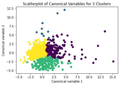
Canonical discriminant analyses was used to reduce the 9 clustering variable down a few variables that accounted for most of the variance in the clustering variables. A scatterplot of the first two canonical variables by cluster (Figure shown below) indicated that the observations in clusters overlap very much with the other clusters.

it s mybe better to do in 3 Clusters

I have changed cluster n in 3 Clusters

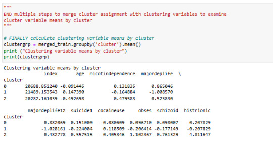
The means on the clustering variables showed that, compared to the other clusters, paranoide mean in cluster 2 is higher .

They had a relatively high likelihood histrionic per.disorder and obsessiv_compulsive Per.disorder. and schizoid per.disorder.

in Cluster 2 is suiside, nicotindependence, cocain use level higher then in other clusters

Cluster 0 has the lowest Paranoide level

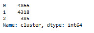
we have to add number of people in each cluster

Cluster (0) 4866

Cluster (1) 4318

Cluster (2) 385

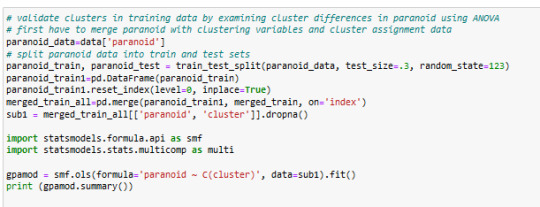
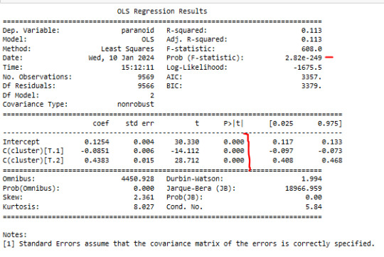
In order to externally validate the clusters, an Analysis of Variance (ANOVA) was conducting to test for significant differences between the clusters on grade paranoide . A tukey test was used for post hoc comparisons between the clusters. Results indicated significant differences between the clusters on paranoide

. The tukey post hoc comparisons showed significant differences between clusters on paranoide.

paranoide in cluster 2 had the highest paranoide (mean=0.563636 sd=0.496579), and cluster 0 had the lowest paranoide (mean=0.040, sd=0.19).

my code below:

code

######################

import numpy as np import matplotlib.pyplot as plt

Definiere die Funktionen

def f1(x): return 2*x + 3

def f2(x): return 3*x + 2

def f3(x): return 4*x + 5

def f4(x): return 5*x + 4

Definiere die Funktion für die Berechnung der neuen Steigung und y-Achsenabschnitt

def adjust_function(f, x_offset): slope = (f(x_offset + 1) - f(x_offset)) / 1 # Berechne die Steigung intercept = f(x_offset) - slope * x_offset # Berechne den y-Achsenabschnitt return lambda x: slope * x + intercept # Neue Funktion mit angepasster Steigung und y-Achsenabschnitt

Wähle den Offset-Punkt

x_offset = 2

Passe die Funktionen an

f1_adjusted = adjust_function(f1, x_offset) f2_adjusted = adjust_function(f2, x_offset) f3_adjusted = adjust_function(f3, x_offset) f4_adjusted = adjust_function(f4, x_offset)

Plotte die Funktionen

x_values = np.linspace(0, 10, 100) plt.plot(x_values, f1_adjusted(x_values), label='f1 adjusted') plt.plot(x_values, f2_adjusted(x_values), label='f2 adjusted') plt.plot(x_values, f3_adjusted(x_values), label='f3 adjusted') plt.plot(x_values, f4_adjusted(x_values), label='f4 adjusted')

plt.xlabel('x') plt.ylabel('f(x)') plt.title('Adjusted linear functions') plt.legend() plt.grid(True) plt.show()

#########

import numpy as np import matplotlib.pyplot as plt

Definiere die Funktionen

def f1(x): return 2*x + 3

def f2(x): return 3*x + 2

def f3(x): if x < 7: return 4x + 5 else: return 2x - 9 # Anpassen der Funktion 3 ab x=7

def f4(x): return 5*x + 4

Definiere die Funktion für die Berechnung der neuen Steigung und y-Achsenabschnitt

Wähle den Offset-Punkt

x_offset = 1

Passe die Funktionen an

f1_adjusted = adjust_function(f1, x_offset) f2_adjusted = adjust_function(f2, x_offset) f3_adjusted = f3 # Funktion 3 wird nicht angepasst, da sie unabhängig sein soll f4_adjusted = adjust_function(f4, x_offset)

Plotte die Funktionen

x_values = np.arange(1, 26) # X-Achse von 1 bis 25 plt.plot(x_values, f1_adjusted(x_values), label='f1 adjusted') plt.plot(x_values, f2_adjusted(x_values), label='f2 adjusted') plt.plot(x_values, f3_adjusted(x_values), label='f3 adjusted') plt.plot(x_values, f4_adjusted(x_values), label='f4 adjusted')

plt.xticks(np.arange(1, 26, 1)) # Setze die Schritte der X-Achse auf 1 plt.xlabel('x') plt.ylabel('f(x)') plt.title('Adjusted linear functions') plt.legend() plt.grid(True) plt.show()

äääääääääää

import numpy as np import matplotlib.pyplot as plt

Definiere die Funktionen

def f1(x): return 2*x + 3

def f2(x): return 3*x + 2

def f3(x): return 4*x + 5

def f4(x): return 5*x + 4

Berechne den Startpunkt für alle Funktionen

x_start = 1 y_start_f1 = f1(x_start) y_start_f2 = f2(x_start) y_start_f3 = f3(x_start) y_start_f4 = f4(x_start)

Definiere die verschobenen Funktionen

def f1_shifted(x): return f1(x) - y_start_f1

def f2_shifted(x): return f2(x) - y_start_f2

def f3_shifted(x): return f3(x) - y_start_f3

def f4_shifted(x): return f4(x) - y_start_f4

Plotte die verschobenen Funktionen

x_values = np.linspace(1, 10, 100) # Annahme eines Bereichs von 1 bis 10 für x plt.plot(x_values, f1_shifted(x_values), label='f1 shifted') plt.plot(x_values, f2_shifted(x_values), label='f2 shifted') plt.plot(x_values, f3_shifted(x_values), label='f3 shifted') plt.plot(x_values, f4_shifted(x_values), label='f4 shifted')

plt.xlabel('x') plt.ylabel('f(x)') plt.title('Shifted linear functions') plt.legend() plt.grid(True) plt.show()

0 notes

infotechall · 4 years ago

Text

K-means clustering analysis

# standardize clustering variables to have mean=0 and sd=1 clustervar=cluster_data.copy() clustervar['ALCOHOL']=preprocessing.scale(clustervar['ALCOHOL'].astype('float64')) clustervar['MALIC_ACID']=preprocessing.scale(clustervar['MALIC_ACID'].astype('float64')) clustervar['ASH']=preprocessing.scale(clustervar['ASH'].astype('float64')) clustervar['ASH_ALCANITY']=preprocessing.scale(clustervar['ASH_ALCANITY'].astype('float64')) clustervar['MAGNESIUM']=preprocessing.scale(clustervar['MAGNESIUM'].astype('float64')) clustervar['TOTAL_PHENOLS']=preprocessing.scale(clustervar['TOTAL_PHENOLS'].astype('float64')) clustervar['FLAVANOIDS']=preprocessing.scale(clustervar['FLAVANOIDS'].astype('float64')) clustervar['NONFLAVANOID_PHENOLS']=preprocessing.scale(clustervar['NONFLAVANOID_PHENOLS'].astype('float64')) clustervar['PROANTHOCYANINS']=preprocessing.scale(clustervar['PROANTHOCYANINS'].astype('float64')) clustervar['COLOR_INTENSITY']=preprocessing.scale(clustervar['COLOR_INTENSITY'].astype('float64')) clustervar['HUE']=preprocessing.scale(clustervar['HUE'].astype('float64')) clustervar['PROLINE']=preprocessing.scale(clustervar['PROLINE'].astype('float64'))from pandas import Series, DataFrame import pandas as pd import numpy as np import os import matplotlib.pylab as plt from sklearn.model_selection import train_test_split from sklearn import preprocessing from sklearn.cluster import KMeans import sklearn.metricsIn this experimental analysis wine dataset were used to apply a K-means clustering analysis. The analysis was performed in order to identify the subgroups of wines based on the similarity of values from 12 variables. Clustering variables were included to identify the types of wines from the all observation variables, and quantitative variables such as Alcohol, Malic-acid, Ash, Alkalinity of ash, Magnesium, Total-phenols, Flavonoids, Non-flavonoid-phenols, Proanthocyanins, Color-intensity, Hue, Proline was included with clustering variables with standardized to have a mean of 0 and a standard deviation of 1.

The dataset was split into a training set that encompasses 70% of the observations(N=124) and a test set that included 30% of the observations (N=55).

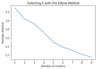
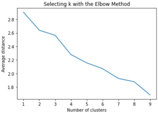
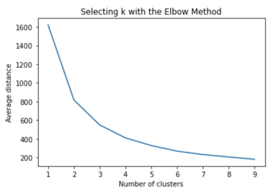
Data were randomly split into a training set that included 70% of the observations (N=3201) and a test set that included 30% of the observations (N=1701). A series of k-means cluster analyses were conducted on the training data specifying k=1-9 clusters, using Euclidean distance. The variance in the clustering variables that was accounted for by the clusters (r-square) was plotted for each of the nine cluster solutions in an elbow curve to provide guidance for choosing the number of clusters to interpret.

Figure 1 Elbow curve of r-square values for the nine cluster solutions

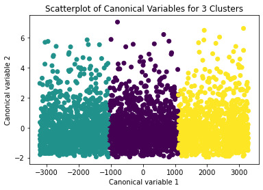
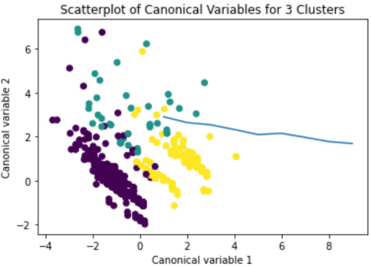
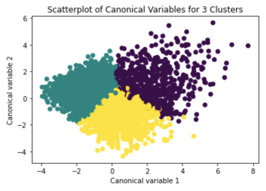
Canonical discriminant analyses were used to reduce the 12-clustering variable down a few variables that used for the most of the variance in the clustering variables

Figure 2 Plot of the first two canonical variables for the clustering variables by cluster

======= ====The following is the python code===================

from pandas import Series, DataFrame import pandas as pd import numpy as np import os import matplotlib.pylab as plt from sklearn.model_selection import train_test_split from sklearn import preprocessing from sklearn.cluster import KMeans import sklearn.metrics

#Data Management os.chdir("E:\Python-works\dataset")

data = pd.read_csv('./wine-clustering.csv')

#upper-case all DataFrame column names data.columns = map(str.upper, data.columns)

# Data Management

data_clean = data.dropna()

# subset clustering variables cluster_data=data_clean[['ALCOHOL','MALIC_ACID','ASH','ASH_ALCANITY','MAGNESIUM', 'TOTAL_PHENOLS','FLAVANOIDS','NONFLAVANOID_PHENOLS','PROANTHOCYANINS', 'COLOR_INTENSITY','HUE','PROLINE']] cluster_data.describe()

# split data into train and test sets clus_train, clus_test = train_test_split(clustervar, test_size=.3, random_state=123)

# k-means cluster analysis for 1-9 clusters from scipy.spatial.distance import cdist clusters=range(1,10) meandist=[]

for k in clusters: model=KMeans(n_clusters=k) model.fit(clus_train) clusassign=model.predict(clus_train) meandist.append(sum(np.min(cdist(clus_train, model.cluster_centers_, 'euclidean'), axis=1)) / clus_train.shape[0])

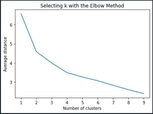
#Plot average distance from observations from the cluster centroid #to use the Elbow Method to identify number of clusters to choose plt.plot(clusters, meandist) plt.xlabel('Number of clusters') plt.ylabel('Average distance') plt.title('Selecting k with the Elbow Method')

# Interpret 3 cluster solution model3=KMeans(n_clusters=3) model3.fit(clus_train) clusassign=model3.predict(clus_train)

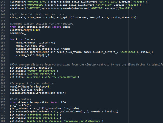
# plot clusters

from sklearn.decomposition import PCA pca_2 = PCA(2) plot_columns = pca_2.fit_transform(clus_train) plt.scatter(x=plot_columns[:,0], y=plot_columns[:,1], c=model3.labels_,) plt.xlabel('Canonical variable 1') plt.ylabel('Canonical variable 2') plt.title('Scatterplot of Canonical Variables for 3 Clusters') plt.show()

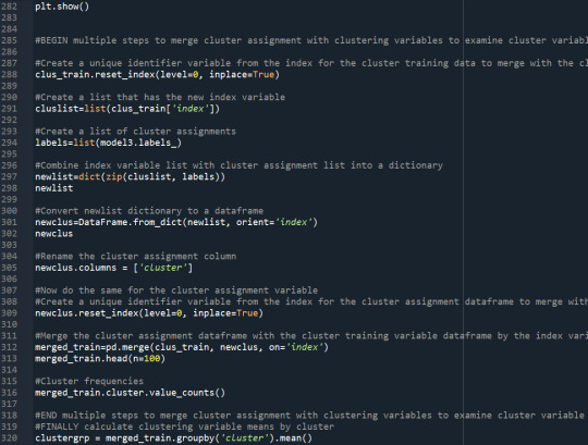
# create a unique identifier variable from the index for the # cluster training data to merge with the cluster assignment variable

clus_train.reset_index(level=0, inplace=True)

# create a list that has the new index variable cluslist=list(clus_train['index'])

# create a list of cluster assignments labels=list(model3.labels_)

# combine index variable list with cluster assignment list into a dictionary newlist=dict(zip(cluslist, labels)) newlist

# convert newlist dictionary to a dataframe newclus=DataFrame.from_dict(newlist, orient='index') newclus

# rename the cluster assignment column newclus.columns = ['cluster']

# now do the same for the cluster assignment variable # create a unique identifier variable from the index for the # cluster assignment dataframe # to merge with cluster training data newclus.reset_index(level=0, inplace=True)

# merge the cluster assignment dataframe with the cluster training variable dataframe # by the index variable merged_train=pd.merge(clus_train, newclus, on='index') merged_train.head(n=100)

# cluster frequencies merged_train.cluster.value_counts()

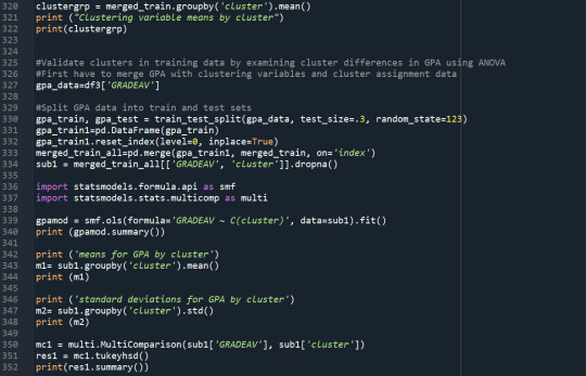
# validate clusters in training data by examining cluster differences in ODR using ANOVA # first have to merge GPA with clustering variables and cluster assignment data gpa_data=data_clean['ODR']

# split GPA data into train and test sets gpa_train, gpa_test = train_test_split(gpa_data, test_size=.3, random_state=123) gpa_train1=pd.DataFrame(gpa_train) gpa_train1.reset_index(level=0, inplace=True) merged_train_all=pd.merge(gpa_train1, merged_train, on='index') sub1 = merged_train_all[['ODR', 'cluster']].dropna()

import statsmodels.formula.api as smf import statsmodels.stats.multicomp as multi

gpamod = smf.ols(formula='ODR ~ C(cluster)', data=sub1).fit() print (gpamod.summary())

print ('means for ODR by cluster') m1= sub1.groupby('cluster').mean() print (m1)

print ('standard deviations for ODR by cluster') m2= sub1.groupby('cluster').std() print (m2)

mc1 = multi.MultiComparison(sub1['ODR'], sub1['cluster']) res1 = mc1.tukeyhsd() print(res1.summary())

#Canonical discriminant analyses were used to reduce the 12-clustering variable down a few variables that used for the most of the variance i #Figure 2 Plot of the first two canonical variables for the clustering variables by cluster

0 notes

rahuljoy-blog2 · 5 years ago

Text

Running a k-means Cluster Analysis

A k-means cluster analysis was conducted to identify underlying subgroups of adolescents based on their similarity of responses on 5 variables that represent characteristics that could have an impact on school achievement. Clustering variables included two binary variables measuring whether or not the adolescent had ever used alcohol or marijuana, as well as quantitative variables measuring alcohol problems, a scale measuring engaging in deviant behaviors (such as vandalism, other property damage, lying, stealing, running away, driving without permission, selling drugs, and skipping school), and scales measuring violence. All clustering variables were standardized to have a mean of 0 and a standard deviation of 1.

Figure 1. Elbow curve of r-square values for the nine cluster solutions

The elbow curve was inconclusive, suggesting that the 2, 3 and 4-cluster solutions might be interpreted. The results below are for an interpretation of the 4-cluster solution.

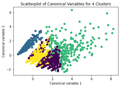
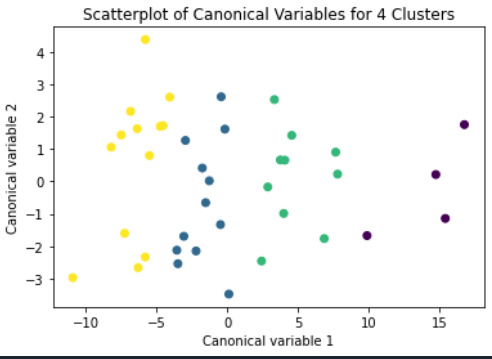
Canonical discriminant analyses was used to reduce the 5 clustering variable down a few variables that accounted for most of the variance in the clustering variables. A scatterplot of the first two canonical variables by cluster is shown in Figure 2 below:

Figure 2. Plot of the first two canonical variables for the clustering variables by cluster

4 notes · View notes

apoorva-week4 · 2 years ago

Text

Week 4: Peer-graded Assignment: Running a k-means Cluster Analysis

This assignment is intended for Coursera course "Machine Learning for Data Analysis by Wesleyan University”.

It is for "Week 4: Peer-graded Assignment: Running a k-means Cluster Analysis".

I am working on k-means Cluster Analysis in Python.

Syntax used to run k-means Cluster Analysis

A k-means cluster analysis was conducted to identify underlying subgroups of real machine parameters based on their similarity of responses on 19 variables that represent characteristics that could have an impact on product yield loss. Clustering variables included only quantitative variables measuring different machine parameters. All clustering variables were standardized to have a mean of 0 and a standard deviation of 1. Data were randomly split into a training set that included 70% of the observations (N=116) and a test set that included 30% of the observations (N=50). A series of k-means cluster analyses were conducted on the training data specifying k=1-9 clusters, using Euclidean distance. The variance in the clustering variables that was accounted for by the clusters (r-square) was plotted for each of the nine cluster solutions in an elbow curve to provide guidance for choosing the number of clusters to interpret.

2. Code used to run k-means Cluster Analysis

3. Corresponding Output

Figure 1. Elbow curve of r-square values for the nine cluster solutions

Figure 2. Plot of the first two canonical variables for the clustering variables by cluster.

4. Interpretation

For Figure 1: The elbow curve was inconclusive, suggesting that the 2, 4 and 8-cluster solutions might be interpreted. All 3 were tested, yielding [F-statistic and Prob (F-statistic)] of: [0.5298,0.469]; [6.242,0.000725] and [3.73,0.00156] accordingly. The results below are for an interpretation of the 4-cluster solution (highest F-statistic and lowest Prob).

Canonical discriminant analyses was used to reduce the 19 clustering variable down a few variables that accounted for most of the variance in the clustering variables. A scatterplot of the first two canonical variables by cluster indicated that the observations in cluster 1 was densely packed with relatively low within cluster variance, and did not overlap very much with the other clusters. Cluster 2 was generally distinct, but the observations had greater spread suggesting higher within cluster variance. Observations in cluster 3 and 4 were spread out more than the other clusters, showing high within cluster variance. The results of this plot suggest that the best cluster solution may have fewer than 4 clusters, so it will be especially important to also evaluate the cluster solutions with fewer than 4 clusters.

For Figure 2: In order to externally validate the clusters, an Analysis of Variance (ANOVA) was conducting to test for significant differences between the clusters on product failure rates (BINS_SUM).

A tukey test was used for post hoc comparisons between the clusters. Results indicated some significant differences between the clusters on BINS_SUM (F (3, 85) = 6.242, p<.0001). The tukey post hoc comparisons showed significant differences between clusters on BINS_SUM for cluster vs. 1 and 3, however insignificance of all other clusters among each other. Samples in cluster 4 had the lowest BINS_SUM (mean=60.28, sd=10.89), and cluster 1 had the highest BINS_SUM (mean=76.35, sd=13.08).

#Running a k-means Cluster Analysis #Machine Learning for Data Analysis #Wesleyan University #Coursera #Python #Week4

0 notes

anuja05 · 3 years ago

Text

A k-means cluster analysis was conducted to identify underlying subgroups of houses based on their similarity of features on 18 variables that represent characteristics of the houses that could have an impact on the grades provided to the house. Clustering variables included price of the house, bedrooms, bathrooms, measurement of the house in square foot, measurement of the lot in square foot, floors, whether a house has a view to waterfront, whether a house has been viewed or not, condition of a house on a scale of 1 to 5, overall grade given to the housing unit based on grading system on a scale of 1 to 11, square footage of house apart from basement, square footage of the basement of the house, years since house is built, years since house is renovated, zip code, latitude, longitude, living room area in 2015, lot size area in 2015. All clustering variables were standardized to have a mean of zero and a standard deviation of one. Data were randomly split into a training set that included 70% of the observations (N= 1145) and a test set that included 30% of the observations (N= 491). A series of k-means cluster analyses were conducted on the training data specifying k=1-9 clusters, using Euclidean distance. The average distance from observations was plotted for each of the nine cluster solutions in an elbow curve to provide guidance for choosing the number of clusters to interpret.

Elbow curve From the below figure, 3 or 4 cluster solutions might be interpreted.

Canonical discriminant analyses was used to reduce the 18 clustering variable down a few variables that accounted for most of the variance in the clustering variables. A scatterplot of the first two canonical variables by cluster (Figure 2 shown below) indicated that the observations in 2 and 3 clusters are densely packed with relatively low within cluster variance and did not overlap very much with the other clusters. Cluster 1 observations had greater spread suggesting higher within cluster variance.

Here the size of cluster 4 is too small also is has higher within cluster variation.

The results of above both plots suggest that the best cluster solution will be 3 clusters.

The means on the clustering variables showed that, compared to the other clusters, houses in cluster 1 had moderate levels on the clustering variables. They had moderate house prices with moderate numbers of bedrooms. The size of the living house is also moderate compared to other clusters. Houses in cluster 2 have low prices compared to other clusters. Even their number of bedrooms and bathrooms, area under living house is low. Exception is the number of years since the house was built is moderate. Cluster 3 can be classified as the expensive and high graded houses as they have the highest price compared to other 2 clusters. Their number of bedrooms and bathrooms, also the living area and the area under the lot is highest. They have highest number of floors along with maximum area in the basement.

In order to externally validate the clusters, an Analysis of Variance (ANOVA) was conducting to test for significant differences between the clusters on grade assigned to these houses. A tukey test was used for post hoc comparisons between the clusters. Results indicated significant differences between the clusters on Grades (p<.0001). The tukey post hoc comparisons showed significant differences between clusters on Grades, with the exception that clusters 1 and 2 were not significantly different from each other. Adolescents in cluster 3 had the highest Grades (mean=1.98, sd=0.83), and cluster 2 had the lowest Grades (mean=1.21, sd=0.44).

Codes-

from pandas import Series, DataFrame

import pandas as pd

import numpy as np

import matplotlib.pylab as plt

from sklearn.cross_validation import train_test_split

from sklearn import preprocessing

from sklearn.cluster import KMeans

"""

Data Management

"""

data = pd.read_csv('kc_house_data.csv')

#upper-case all DataFrame column names

data.columns = map(str.upper, data.columns)

# subset clustering variables

cluster=data[['PRICE','BEDROOMS','BATHROOMS','SQFT_LIVING','SQFT_LOT','FLOORS','WATERFRONT',

'VIEW','CONDITION','SQFT_ABOVE','SQFT_BASEMENT','YR_BUILT','YR_RENOVATED','ZIPCODE',

'LAT','LONG','SQFT_LIVING15','SQFT_LOT15']]

cluster.describe()

# standardize clustering variables to have mean=0 and sd=1

clustervar=cluster.copy()

from sklearn import preprocessing

clustervar['PRICE']=preprocessing.scale(clustervar['PRICE'].astype('float64'))

clustervar['BEDROOMS']=preprocessing.scale(clustervar['BEDROOMS'].astype('float64'))

clustervar['BATHROOMS']=preprocessing.scale(clustervar['BATHROOMS'].astype('float64'))

clustervar['SQFT_LIVING']=preprocessing.scale(clustervar['SQFT_LIVING'].astype('float64'))

clustervar['SQFT_LOT']=preprocessing.scale(clustervar['SQFT_LOT'].astype('float64'))

clustervar['FLOORS']=preprocessing.scale(clustervar['FLOORS'].astype('float64'))

clustervar['WATERFRONT']=preprocessing.scale(clustervar['WATERFRONT'].astype('float64'))

clustervar['VIEW']=preprocessing.scale(clustervar['VIEW'].astype('float64'))

clustervar['CONDITION']=preprocessing.scale(clustervar['CONDITION'].astype('float64'))

clustervar['SQFT_ABOVE']=preprocessing.scale(clustervar['SQFT_ABOVE'].astype('float64'))

clustervar['SQFT_BASEMENT']=preprocessing.scale(clustervar['SQFT_BASEMENT'].astype('float64'))

clustervar['YR_BUILT']=preprocessing.scale(clustervar['YR_BUILT'].astype('float64'))

clustervar['YR_RENOVATED']=preprocessing.scale(clustervar['YR_RENOVATED'].astype('float64'))

clustervar['ZIPCODE']=preprocessing.scale(clustervar['ZIPCODE'].astype('float64'))

clustervar['LAT']=preprocessing.scale(clustervar['LAT'].astype('float64'))

clustervar['LONG']=preprocessing.scale(clustervar['LONG'].astype('float64'))

clustervar['SQFT_LIVING15']=preprocessing.scale(clustervar['SQFT_LIVING15'].astype('float64'))

clustervar['SQFT_LOT15']=preprocessing.scale(clustervar['SQFT_LOT15'].astype('float64'))

# split data into train and test sets

clus_train, clus_test = train_test_split(clustervar, test_size=.3, random_state=123)

# k-means cluster analysis for 1-9 clusters

from scipy.spatial.distance import cdist

clusters=range(1,10)

meandist=[]

for k in clusters:

model=KMeans(n_clusters=k)

model.fit(clus_train)

clusassign=model.predict(clus_train)

meandist.append(sum(np.min(cdist(clus_train, model.cluster_centers_, 'euclidean'), axis=1))

/ clus_train.shape[0])

"""

Plot average distance from observations from the cluster centroid

to use the Elbow Method to identify number of clusters to choose

"""

plt.plot(clusters, meandist)

plt.xlabel('Number of clusters')

plt.ylabel('Average distance')

plt.title('Selecting k with the Elbow Method')

# Interpret 3 cluster solution

model3=KMeans(n_clusters=3)

model3.fit(clus_train)

clusassign=model3.predict(clus_train)

# plot clusters

from sklearn.decomposition import PCA

pca_2 = PCA(2)

plot_columns = pca_2.fit_transform(clus_train)

plt.scatter(x=plot_columns[:,0], y=plot_columns[:,1], c=model3.labels_,)

plt.xlabel('Canonical variable 1')

plt.ylabel('Canonical variable 2')

plt.title('Scatterplot of Canonical Variables for 3 Clusters')

plt.show()

"""

BEGIN multiple steps to merge cluster assignment with clustering variables to examine

cluster variable means by cluster

"""

# create a unique identifier variable from the index for the

# cluster training data to merge with the cluster assignment variable

clus_train.reset_index(level=0, inplace=True)

# create a list that has the new index variable

cluslist=list(clus_train['index'])

# create a list of cluster assignments

labels=list(model3.labels_)

# combine index variable list with cluster assignment list into a dictionary

newlist=dict(zip(cluslist, labels))

newlist

# convert newlist dictionary to a dataframe

newclus=DataFrame.from_dict(newlist, orient='index')

newclus

# rename the cluster assignment column

newclus.columns = ['cluster']

# now do the same for the cluster assignment variable

# create a unique identifier variable from the index for the

# cluster assignment dataframe

# to merge with cluster training data

newclus.reset_index(level=0, inplace=True)

# merge the cluster assignment dataframe with the cluster training variable dataframe

# by the index variable

merged_train=pd.merge(clus_train, newclus, on='index')

merged_train.head(n=100)

# cluster frequencies

merged_train.cluster.value_counts()

"""

END multiple steps to merge cluster assignment with clustering variables to examine

cluster variable means by cluster

"""

# FINALLY calculate clustering variable means by cluster

clustergrp = merged_train.groupby('cluster').mean()

print ("Clustering variable means by cluster")

print(clustergrp)

# validate clusters in training data by examining cluster differences in GRADE using ANOVA

# first have to merge GRADE with clustering variables and cluster assignment data

GRADE_data=data['GRADE']

# split GPA data into train and test sets

GRADE_train, GRADE_test = train_test_split(GRADE_data, test_size=.3, random_state=123)

GRADE_train1=pd.DataFrame(GRADE_train)

GRADE_train1.reset_index(level=0, inplace=True)

merged_train_all=pd.merge(GRADE_train1, merged_train, on='index')

sub1 = merged_train_all[['GRADE', 'cluster']].dropna()

import statsmodels.formula.api as smf

import statsmodels.stats.multicomp as multi

GRADEmod = smf.ols(formula='GRADE ~ C(cluster)', data=sub1).fit()

print (GRADEmod.summary())

print ('means for GRADE by cluster')

m1= sub1.groupby('cluster').mean()

print (m1)

print ('standard deviations for GRADE by cluster')

m2= sub1.groupby('cluster').std()

print (m2)

mc1 = multi.MultiComparison(sub1['GRADE'], sub1['cluster'])

res1 = mc1.tukeyhsd()

print(res1.summary())

print ('standard deviations for GPA by cluster')

m2= sub1.groupby('cluster').std()

print (m2)

mc1 = multi.MultiComparison(sub1['GPA1'], sub1['cluster'])

res1 = mc1.tukeyhsd()

print(res1.summary())

0 notes

zeenahawamdeh · 3 years ago

Text

Running a k-means Cluster Analysis

A k-means cluster analysis was conducted to identify underlying subgroups of lifestyles/habits based on 14 variables. Clustering variables included quantitative variables measuring

INCOME PER PERSON, ALC CONSUMPTION, ARMED FORCES RATE, BREAST CANCER PER 100TH. CO2 EMISSIONS, FEMALE EMPLOYRATE, HIV RATE, INTERNET USE RATE, OIL PER PERSON, POLITY SCORE, ELECTRIC PER PERSON, SUICIDE PER 100TH, EMPLOY RATE, URBAN RATE

All clustering variables were standardized to have a mean of 0 and a standard deviation of 1.

Data were randomly split into a training set that included 70% of the observations (N=39) and a test set that included 30% of the observations (N=17). A series of k-means cluster analyses were conducted on the training data specifying k=1-9 clusters, using Euclidean distance. The variance in the clustering variables that was accounted for by the clusters (r-square) was plotted for each of the nine cluster solutions in an elbow curve to provide guidance for choosing the number of clusters to interpret.

Figure 1. Elbow curve of r-square values for the nine cluster solutions

The elbow curve was inconclusive, suggesting that the 2 and 4 cluster solutions might be interpreted. The results below are for an interpretation of the 4-cluster solution.

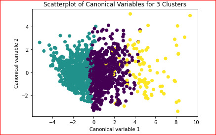
Canonical discriminant analyses was used to reduce the 14 clustering variable down a few variables that accounted for most of the variance in the clustering variables. A scatterplot of the first two canonical variables by cluster (Figure 2 shown below) indicated that the observations in clusters 1 through 4 were distinct and did not overlap with the other clusters. Observations in cluster 4 or deep red were spread out more than the other clusters, showing high within cluster variance.

Figure 2. Plot of the first two canonical variables for the clustering variables by cluster.

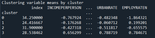
The means on the clustering variables showed that, compared to the other clusters, cluster 1 had highest HIV Rate and cluster 4 had the income per person, highest urban rate, employ rate, oil per person, electric per person and internet use rate. All in all cluster 4 had a better life and thus higher life expectancy was evident. And higher HIV RATE points to lower life expectancy.

In order to externally validate the clusters, an Analysis of Variance (ANOVA) was conducting to test for significant differences between the clusters on LIFE EXPECTANCY. A tukey test was used for post hoc comparisons between the clusters. The tukey post hoc comparisons showed significant differences between clusters on, LIFE EXPECTANCY with the exception that clusters 2 and 3 were not significantly different from each other. People in cluster 4 had the highest LIFE EXPECTANCY (mean=78.06, sd=4.6), and cluster 1 had the lowest LIFE EXPECTANCY (mean=68.25, sd=10.31).

0 notes

arpitabathija · 3 years ago

Text

Assignment 4

A k-means cluster analysis was conducted to identify underlying subgroups of lifestyles/habits based on 14 variables. Clustering variables included quantitative variables measuring

All clustering variables were standardized to have a mean of 0 and a standard deviation of 1.

Figure 1. Elbow curve of r-square values for the nine cluster solutions

The elbow curve was inconclusive, suggesting that the 2 and 4 cluster solutions might be interpreted. The results below are for an interpretation of the 4-cluster solution.

Figure 2. Plot of the first two canonical variables for the clustering variables by cluster.

0 notes

shareyourdatawithme · 3 years ago

Text

Machine Learning - Week 4

This is the fourth and final week of the Machine Learning course, and in this week’s assignment we are tasked with conducting a k-means cluster analysis. The analysis was conducted to identify underlying subgroups of adolescents based on their similarity of responses on 7 variables. The variables represent characteristics that could have an impact on school achievement measured as GPA. Clustering variables included if marijuana was ever used, alcohol problems, gender, depression, self-esteem, if they have ever been expelled, and if they have ever used cocaine. All clustering variables were standardized to have a mean of 0 and a standard deviation of 1.

Data was randomly split into a training set that included 70% of the observations (N=3,202) and a test set that included 30% of the observations (N=1,373). A series of k-means cluster analyses were conducted on the training data specifying k=1-9 clusters, using Euclidean distance. The variance in the clustering variables that was accounted for by the clusters (r-square) was plotted for each of the nine cluster solutions in an elbow curve to provide guidance for choosing the number of clusters to interpret. The figure below is of the elbow curve.

The elbow curve was inconclusive, suggesting that the 2, 3 and 5-cluster solutions might be interpreted. The rest of the analysis was conducted with an interpretation of the 3-cluster solution.

A scatterplot of the first two canonical variables by cluster (Figure below) indicated that the observations in all the clusters had no overlap.

The means on the clustering variables showed that, compared to the other clusters, adolescents in cluster 1 had moderate levels on the clustering variables. They had a relatively low likelihood of using alcohol or marijuana, but moderate levels of depression and self-esteem. With the exception of having a high likelihood of having used alcohol or marijuana, cluster 2 had higher levels on the clustering variables compared to cluster 1.

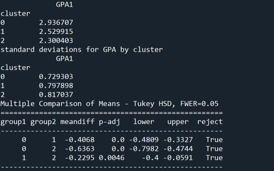
In order to externally validate the clusters, an Analysis of Variance (ANOVA) was conducting to test for significant differences between the clusters on grade point average (GPA). A tukey test was used for post hoc comparisons between the clusters. Results indicated significant differences between the clusters on GPA (F=113.7, p=1.98e-48 – very small).

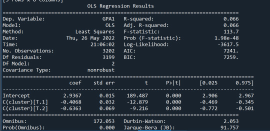
The tukey post hoc comparisons showed significant differences between clusters on GPA. Cluster 3 had the lowest GPA at 2.3 followed by cluster 2 at 2.5. The results of the tukey test indicated that all of the clusters were not significantly different from one another.

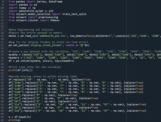
from pandas import Series, DataFrame

import pandas as pd

import numpy as np

import matplotlib.pylab as plt

from sklearn.model_selection import train_test_split

from sklearn import preprocessing

from sklearn.cluster import KMeans

import os

"""

Data Management

"""

os.chdir("C:\TREES")

data = pd.read_csv("tree_addhealth.csv")

#upper-case all DataFrame column names

data.columns = map(str.upper, data.columns)

# Data Management

data_clean = data.dropna()

# subset clustering variables

cluster=data_clean[['BIO_SEX','MAREVER1','ALCPROBS1','COCEVER1',

'DEP1','ESTEEM1','EXPEL1']]

cluster.describe()

# standardize clustering variables to have mean=0 and sd=1

clustervar=cluster.copy()

clustervar['BIO_SEX']=preprocessing.scale(clustervar['BIO_SEX'].astype('float64'))

clustervar['ALCPROBS1']=preprocessing.scale(clustervar['ALCPROBS1'].astype('float64'))

clustervar['MAREVER1']=preprocessing.scale(clustervar['MAREVER1'].astype('float64'))

clustervar['DEP1']=preprocessing.scale(clustervar['DEP1'].astype('float64'))

clustervar['ESTEEM1']=preprocessing.scale(clustervar['ESTEEM1'].astype('float64'))

clustervar['EXPEL1']=preprocessing.scale(clustervar['EXPEL1'].astype('float64'))

clustervar['COCEVER1']=preprocessing.scale(clustervar['COCEVER1'].astype('float64'))

# split data into train and test sets

clus_train, clus_test = train_test_split(clustervar, test_size=.3, random_state=123)

# k-means cluster analysis for 1-9 clusters

from scipy.spatial.distance import cdist

clusters=range(1,10)

meandist=[]

for k in clusters:

model=KMeans(n_clusters=k)

model.fit(clus_train)

clusassign=model.predict(clus_train)

meandist.append(sum(np.min(cdist(clus_train, model.cluster_centers_, 'euclidean'), axis=1))

/ clus_train.shape[0])

"""

Plot average distance from observations from the cluster centroid

to use the Elbow Method to identify number of clusters to choose

"""

plt.plot(clusters, meandist)

plt.xlabel('Number of clusters')

plt.ylabel('Average distance')

plt.title('Selecting k with the Elbow Method')

# Interpret 3 cluster solution

model3=KMeans(n_clusters=3)

model3.fit(clus_train)

clusassign=model3.predict(clus_train)

# plot clusters

from sklearn.decomposition import PCA

pca_2 = PCA(2)

plot_columns = pca_2.fit_transform(clus_train)

plt.scatter(x=plot_columns[:,0], y=plot_columns[:,1], c=model3.labels_,)

plt.xlabel('Canonical variable 1')

plt.ylabel('Canonical variable 2')

plt.title('Scatterplot of Canonical Variables for 3 Clusters')

plt.show()

"""

BEGIN multiple steps to merge cluster assignment with clustering variables to examine

cluster variable means by cluster

"""

# create a unique identifier variable from the index for the

# cluster training data to merge with the cluster assignment variable

clus_train.reset_index(level=0, inplace=True)

# create a list that has the new index variable

cluslist=list(clus_train['index'])

# create a list of cluster assignments

labels=list(model3.labels_)

# combine index variable list with cluster assignment list into a dictionary

newlist=dict(zip(cluslist, labels))

newlist

# convert newlist dictionary to a dataframe

newclus=DataFrame.from_dict(newlist, orient='index')

newclus

# rename the cluster assignment column

newclus.columns = ['cluster']

# now do the same for the cluster assignment variable

# create a unique identifier variable from the index for the

# cluster assignment dataframe

# to merge with cluster training data

newclus.reset_index(level=0, inplace=True)

# merge the cluster assignment dataframe with the cluster training variable dataframe

# by the index variable

merged_train=pd.merge(clus_train, newclus, on='index')

merged_train.head(n=100)

# cluster frequencies

merged_train.cluster.value_counts()

"""

END multiple steps to merge cluster assignment with clustering variables to examine

cluster variable means by cluster

"""

# FINALLY calculate clustering variable means by cluster

clustergrp = merged_train.groupby('cluster').mean()

print ("Clustering variable means by cluster")

print(clustergrp)

# validate clusters in training data by examining cluster differences in GPA using ANOVA

# first have to merge GPA with clustering variables and cluster assignment data

gpa_data=data_clean['GPA1']

# split GPA data into train and test sets

gpa_train, gpa_test = train_test_split(gpa_data, test_size=.3, random_state=123)

gpa_train1=pd.DataFrame(gpa_train)

gpa_train1.reset_index(level=0, inplace=True)

merged_train_all=pd.merge(gpa_train1, merged_train, on='index')

sub1 = merged_train_all[['GPA1', 'cluster']].dropna()

import statsmodels.formula.api as smf

import statsmodels.stats.multicomp as multi

gpamod = smf.ols(formula='GPA1 ~ C(cluster)', data=sub1).fit()

print (gpamod.summary())

print ('means for GPA by cluster')

m1= sub1.groupby('cluster').mean()

print (m1)

print ('standard deviations for GPA by cluster')

m2= sub1.groupby('cluster').std()

print (m2)

mc1 = multi.MultiComparison(sub1['GPA1'], sub1['cluster'])

res1 = mc1.tukeyhsd()

print(res1.summary())

0 notes

panospaterakis · 3 years ago

Text

Machine Learning for Data Analysis - Week 4

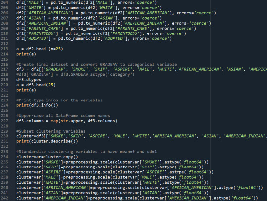
Assignment: Response variable: Excellent average gradeExplanatory variables: Systematic Smoking, Skipping school, Educational aspirations, Gender, White, African American, Asian, American Indian, Parents' education level, Parents' Care, being Adopted You will check the code that I used for this week's assignment below:

Code:

Results:

Summary of the k-means cluster analysis

A k-means cluster analysis was conducted to identify underlying subgroups of adolescents based on their similarity of responses on 11 variables that represent characteristics that could impact school achievement. Clustering variables included The following explanatory variables were included systematic smoking, skipping school, educational aspirations, gender, White, African American, Asian, American Indian, parents' educational level, parents' caring level, and being adopted. All clustering variables were standardized to have a mean of 0 and a standard deviation of 1.

Data were randomly split into a training set that included 70% of the observations (N=990) and a test set that included 30% of the observations (N=425). A series of k-means cluster analyses were conducted on the training data specifying k=1-9 clusters, using Euclidean distance. The variance in the clustering variables that was accounted for by the clusters (r-square) was plotted for each of the nine cluster solutions in an elbow curve to provide guidance for choosing the number of clusters to interpret.

Figure 1. Elbow curve of r-square values for the nine cluster solutions

The elbow curve was inconclusive, suggesting that the 2, 3, 4 and 8-cluster solutions might be interpreted. The results below are for an interpretation of the 3-cluster solution.

Figure 2. Plot of the first two canonical variables for the clustering variables by cluster.

The means on the clustering variables showed that, compared to the other clusters, adolescents in cluster 1 had a relatively high likelihood of smoking and skipping school daily and a lower likelihood of having parents that have finished tertiary education. On the other hand, cluster 2 and 3 had approximately the same likelihood of smoking and skipping school daily, while students in cluster 2 have a higher likelihood to have parents with tertiary education.

In order to externally validate the clusters, an Analysis of Variance (ANOVA) was conducted to test for significant differences between the clusters on excellent grade point average (GPA). A tukey test was used for post hoc comparisons between the clusters. Results indicated significant differences between the clusters on excellent GPA (F-stat=11.88, p<0.01). The tukey post hoc comparisons showed significant differences between clusters on excellent GPA, with the exception that clusters 1 and 2 were not significantly different from each other. Students in cluster 3 had the highest chance to receive an excellent average grade (mean=0.42, sd=0.49), and students in cluster 1 had the lowest (mean=0.19, sd=0.39).

0 notes

friwrite · 4 years ago

Text

Capstone project Draft 3

Preliminary Results

To create the predictor variable it was observed in the different classes their statistical distribution. For example, the PSD of the different tasks(Figure 2) can provide information about the correlation between Movement, Imaginary and Baseline information of all the 10 features extracted. . In previous works of EEG classification is mentioned that correlation between imagery and motor signals can contribute to the performance of a BCI.

Figure 1. PSD of S1 and 3 tasks.

In the K-means cluster analysis, the variance in the clustering variables that was accounted for by the clusters (r-square) was plotted for each of the nine cluster solutions in an elbow curve to provide guidance for choosing the number of clusters to interpret.

Figure 2. Elbow curve of r-square values for the nine cluster solutions

The elbow curve was inconclusive, suggesting that the 2, 4 and 5-cluster solutions might be interpreted. The results below are for an interpretation of the 2-cluster solution.

Canonical discriminant analyses was used to reduce the 10 clustering variable down a few variables that accounted for most of the variance in the clustering variables. A scatterplot of the first two canonical variables by cluster (Figure 2 shown below) indicated that the observations in clusters 1 and 2 were densely packed with relatively low within cluster variance, and did not overlap very much with the other clusters. Cluster 2 was generally distinct, but the observations had greater spread suggesting higher within cluster variance. The results of this plot suggest that the best cluster solution may have fewer than 3 clusters, so it will be especially important to also evaluate the cluster solutions with fewer than 4 clusters.

Figure 3. Plot of the first two canonical variables for the clustering variables by cluster.

The means on the clustering variables showed that, compared to the other clusters, values in cluster 1 had moderate levels on the clustering variables. They had a relatively low percentage to belong to a inactivity class.

In order to externally validate the clusters, an Analysis of Variance (ANOVA) was conducting to test for significant differences between the clusters on the target variable. A tukey test was used for post hoc comparisons between the clusters. Results indicated significant differences between the clusters on target variable(80.4, p<.0001). The tukey post hoc comparisons showed significant differences between clusters on the target variable, with the exception that clusters 1 and 2 were not significantly different from each other. Values in cluster 1 had the highest value(mean= -0.0278 , sd=0.81), and cluster 2 had the lowest GPA (mean=-0.2496 , sd=0.19).

For the Random Forest analysis the explanatory variables with the highest relative importance scores were Shannon and the DWT. The accuracy of the random forest was nearly 100% (97.96%) after 25 decision trees (Figure 3) adding little to the overall accuracy of the model, (that was aprox 94%) and suggesting that interpretation of a single decision tree may be appropriate.

Note: Each trainning of a Random Forest, increases the accuracy of the model.

Figure 4. Random Forest accuracy after 25 decision trees

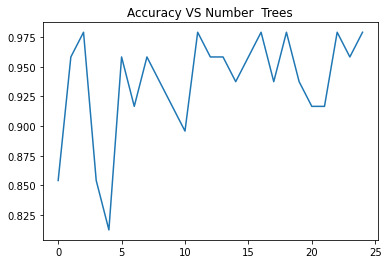
Table 1 compares the accuracy for machine learning algorithms of all the available features and pairs of features chosen by their importance for the system. The first column portrays the best percentage of accuracy and corresponds to all the available features. The last column shows the features (Shannon Entropy and Discrete Wavelet Transform pair) that compete with the first column performance. A significant difference in accuracy can be observed depending on the conforming of the selected pairs. The pairs of features which algorithms accuracy compete with the use of all the extracted features are the ones with major relevance for the system

Table 1. MI classification with ML algorithms comparison

0 notes

mymlstudies · 4 years ago

Text

K-means Titanic

k-means cluster analysis was conducted to identify underlying subgroups of test data in the Kaggle titanic survival simulation scenario.

based on few passenger records on 4~6 variables that can possibly predict survivability on the titanic event.

Clustering variables measuring whether or not a passenger would be survived. Variables are Age, Fare, Embarked, Class, Sex, and Siblings. All clustering variables were standardized to have a mean of 0 and a standard deviation of 1.

Data were randomly split into a training set that included 70% of the observations (N=499) and a test set that included 30%. A series of k-means cluster analyses were conducted on the training data specifying k=1-9 clusters, using Euclidean distance. The variance in the clustering variables that was accounted for by the clusters (r-square) was plotted for each of the nine cluster solutions in an elbow curve to provide guidance for choosing the number of clusters to interpret.

Figure 1. Elbow curve of r-square values for the nine cluster solutions

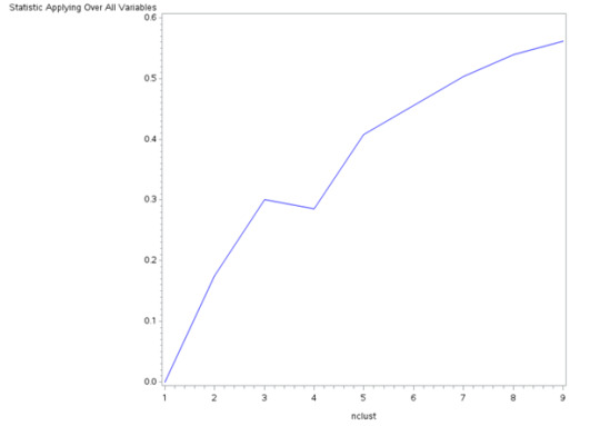
The elbow curve was inconclusive, suggesting that the 3 and 4-cluster solutions might be interpreted. The results below are for an interpretation of the 4-cluster solution.

Figure 2. Plot of the first two canonical variables for the clustering variables by cluster.

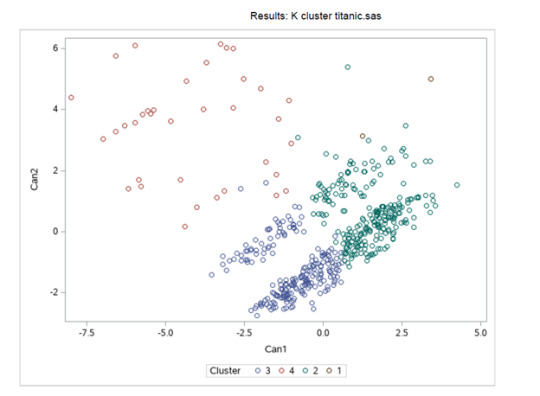
Canonical discriminant analyses were used to reduce the 9-clustering variable down a few variables that accounted for most of the variance in the clustering variables. A scatterplot of the first two canonical variables by cluster (Figure 2 shown below) indicated that the observations in clusters 2 and 3 were densely packed with relatively low within cluster variance, and did not overlap very much with the other clusters. Cluster 1 was generally distinct, but the observations had greater spread suggesting higher within cluster variance. Observations in cluster 4 were spread out more than the other clusters, showing high within cluster variance. The results of this plot suggest that the best cluster solution may have fewer than 4 clusters, so it will be especially important to also evaluate the cluster solutions with only 2 clusters.

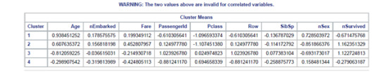
The means on the clustering variables showed that, compared to the other clusters, nSurvived in cluster 2 and 3 had more chances to survived on the clustering variables. Compared to other clusters with less than 1 cluster means. Does having these groups with nSex closer to be with more composed of men and less likely to have siblings on board. Also with age group on the mid ranges. While Embarked, Fare, and Pclass shows no apparent significance.

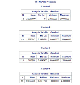
In order to externally validate the clusters, an Analysis of Variance (ANOVA) was conducting to test for significant differences between the clusters on nSurvived. Cluster 1 is neglected due to its few sample size.

SAS Code Used:

data clust;

set SASUSER.titanic;

if Sex="male" then nSex=2;

if Sex="female" then nSex=1;

if Embarked="S" then nEmbarked=1;

if Embarked="C" then nEmbarked=2;

if Embarked="Q" then nEmbarked=3;

if Survived=0 then nSurvived=1;

if Survived=1 then nSurvived=2;

idnum=_n_;

keep idnum Age nEmbarked Fare PassengerId Pclass Row nSex SibSp nSurvived;

if cmiss(of _all_) then delete;

run;

ods graphics on;

proc surveyselect data=clust out=traintest seed = 123

samprate=0.7 method=srs outall;

run;

data clus_train;

set traintest;

if selected=1;

run;

data clus_test;

set traintest;

if selected=0;

run;

proc standard data=clus_train out=clustvar mean=0 std=1;

var Age nEmbarked Fare PassengerId Pclass Row nSex SibSp nSurvived;

run;

%macro kmean(K);

proc fastclus data=clustvar out=outdata&K. outstat=cluststat&K. maxclusters= &K. maxiter=300;

var Age nEmbarked Fare PassengerId Pclass Row SibSp nSex nSurvived;

run;

%mend;

%kmean(1);

%kmean(2);

%kmean(3);

%kmean(4);

%kmean(5);

%kmean(6);

%kmean(7);

%kmean(8);

%kmean(9);

data clus1;

set cluststat1;

nclust=1;

if _type_='RSQ';

keep nclust over_all;

run;

data clus2;

set cluststat2;

nclust=2;

if _type_='RSQ';

keep nclust over_all;

run;

data clus3;

set cluststat3;

nclust=3;

if _type_='RSQ';

keep nclust over_all;

run;

data clus4;

set cluststat4;

nclust=4;

if _type_='RSQ';

keep nclust over_all;

run;

data clus5;

set cluststat5;

nclust=5;

if _type_='RSQ';

keep nclust over_all;

run;

data clus6;

set cluststat6;

nclust=6;

if _type_='RSQ';

keep nclust over_all;

run;

data clus7;

set cluststat7;

nclust=7;

if _type_='RSQ';

keep nclust over_all;

run;

data clus8;

set cluststat8;

nclust=8;

if _type_='RSQ';

keep nclust over_all;

run;

data clus9;

set cluststat9;

nclust=9;

if _type_='RSQ';

keep nclust over_all;

run;

data clusrsquare;

set clus1 clus2 clus3 clus4 clus5 clus6 clus7 clus8 clus9;

run;

* plot elbow curve using r-square values;

symbol1 color=blue interpol=join;

proc gplot data=clusrsquare;

plot over_all*nclust;

run;

* plot clusters for 4 cluster solution;

proc candisc data=outdata4 out=clustcan;

class cluster;

var Age nEmbarked Fare PassengerId Pclass Row SibSp nSex nSurvived;

run;

proc sgplot data=clustcan;

scatter y=can2 x=can1 / group=cluster;

run;

* validate clusters on GPA;

* first merge clustering variable and assignment data with GPA data;

data gpa_data;

set clus_train;

keep idnum SVD1;

run;

proc sort data=outdata4;

by idnum;

run;

proc sort data=SVD_data;

by idnum;

run;

data merged;

merge outdata4 SVD_data;

by idnum;

run;

proc sort data=merged;

by cluster;

run;

proc means data=merged;

var SVD1;

by cluster;

run;

proc anova data=merged;

class cluster;

model SVD1 = cluster;

means cluster/tukey;

run;

Thanks for reading!!!

0 notes

sarahayton · 4 years ago

Text

Running a k-means Cluster Analysis

A k-means cluster analysis was conducted to identify subgroups of people based on their similarity across 16 variables that might have an impact on marijuana use. Clustering variables included a number of characteristics including: age, alcohol and other substance use (ALCEVR1, ALCPROBS1, COCEVER1, INHEVER1), behavioral (DEP1, ESTEEM1, VIOL1), as well as educational (DEVIANT1, GPA1, EXPEL1) and family (FAMCONCT, PARACTV, PARPRES) characteristics. All predictors were standardized to have a mean value of zero and a standard deviation of one.

data = pd.read_csv("tree_addhealth.csv")

cluster=data_clean[['AGE', 'ALCEVR1', 'ALCPROBS1', 'COCEVER1', 'INHEVER1', 'CIGAVAIL', 'DEP1', 'ESTEEM1', 'VIOL1', 'PASSIST', 'DEVIANT1', 'GPA1', 'EXPEL1', 'FAMCONCT','PARACTV', 'PARPRES']]

Data were randomly split into a training set that included 70% of the observationsand a test set that included 30% of the observations. A series of k-means cluster analyses were conducted on the training data specifying k=1-9 clusters, using Euclidean distance. The variance in the clustering variables that was accounted for by the clusters (r-square) was plotted for each of the nine cluster solutions in an elbow curve to provide guidance for choosing the number of clusters to interpret.

clus_train, clus_test = train_test_split(clustervar, test_size=.3, random_state=123)

from scipy.spatial.distance import cdist

clusters=range(1,10)

meandist=[]

for k in clusters:

model=KMeans(n_clusters=k)

model.fit(clus_train)

clusassign=model.predict(clus_train)

meandist.append(sum(np.min(cdist(clus_train, model.cluster_centers_, 'euclidean'), axis=1)) / clus_train.shape[0])

plt.plot(clusters, meandist)

plt.xlabel('Number of clusters')

plt.ylabel('Average distance')

plt.title('Selecting k with the Elbow Method')

Figure 1. Elbow curve of r-square values for the nine cluster solutions

The elbow curve was inconclusive, suggesting that the 2 and 3-cluster solutions might be interpreted. The results below are for an interpretation of the 3-cluster solution.

Canonical discriminant analyses was used to reduce the 16 clustering variable down a few variables that accounted for most of the variance in the clustering variables. A scatterplot of the first two canonical variables by cluster (Figure 2 shown below) indicated that the observations in clusters 1 and 4 were densely packed with relatively low within cluster variance, and did not overlap very much with the other clusters. Cluster 2 was generally distinct, but the observations had greater spread suggesting higher within cluster variance. Observations in cluster 3 were spread out more than the other clusters, showing high within cluster variance. The results of this plot suggest that the best cluster solution may have fewer than 4 clusters, so it will be especially important to also evaluate the cluster solutions with fewer than 4 clusters.

model3=KMeans(n_clusters=3)

model3.fit(clus_train)

clusassign=model3.predict(clus_train)

pca_2 = PCA(2)

Figure 2. Plot of the first two canonical variables for the clustering variables by cluster.

clustergrp = merged_train.groupby('cluster').mean()

print ("Clustering variable means by cluster")

print(clustergrp)

Clustering variable means by cluster

cluster

AGE ALCEVR1 ALCPROBS1 COCEVER1 \

0 17.007748 0.685719 0.981627 0.109325

1 15.053934 -0.448153 -0.340980 0.008289

2 17.758390 0.129689 -0.161056 0.015962

INHEVER1 CIGAVAIL DEP1 ESTEEM1 VIOL1 PASSIST DEVIANT1 \

0 0.180064 0.446945 0.849564 -0.660382 0.830998 0.146302 1.178689

1 0.039940 0.229088 -0.310095 0.244037 -0.170265 0.092690 -0.366272

2 0.039106 0.292897 -0.139679 0.118059 -0.254260 0.091780 -0.220419

GPA1 EXPEL1 FAMCONCT PARACTV PARPRES

0 2.401125 0.098071 -1.096106 -0.439664 -0.563944

1 2.997048 0.017332 0.329184 0.114663 0.149519

2 2.835129 0.031923 0.220210 0.113718 0.132120

The means on the clustering variables showed that, compared to the other clusters, those in cluster 1 had the highest levels of alcohol use, alcohol problems, cocaine use, cigarette access and smoking, depression, violence, deviant behavior, and expulsion. This cluster also had the lowest self esteem, GPA, family connectedness, and parental presence. Those in cluster 2 were younger and had the lowest levels of prior alcohol or substance use, lowest levels of depression and expulsion, and the highest levels of self esteem and GPA. Those in cluster 3 clearly were the oldest and least violent, and fell between clusters 1 and 2 in all other characteristics.

m1= sub1.groupby('cluster').mean()

MAREVER1 cluster

0 0.612540

1 0.086662

2 0.223464

gpamod = smf.ols(formula='MAREVER1 ~ C(cluster)', data=sub1).fit()

mc1 = multi.MultiComparison(sub1['MAREVER1'], sub1['cluster'])

res1 = mc1.tukeyhsd()

Multiple Comparison of Means - Tukey HSD, FWER=0.05 =================================================== group1 group2 meandiff p-adj lower upper reject

---------------------------------------------------

0 1 -0.5259 0.001 -0.5696 -0.4822 True

0 2 -0.3891 0.001 -0.4332 -0.345 True

1 2 0.1368 0.001 0.1014 0.1722 True

---------------------------------------------------

In order to externally validate the clusters, an Analysis of Variance (ANOVA) was conducting to test for significant differences between the clusters on marijuana use. A tukey test was used for post hoc comparisons between the clusters. The tukey post hoc comparisons showed significant differences between all clusters on marijuana use (all p < 0.001). Those in cluster 1 had the highest marijuana use (mean=0.6125, sd=0.4876), and cluster 2 had the lowest marijuana use (mean=0.0866, sd=0.2814).

0 notes

ghaida-2525 · 4 years ago

Text

Running a k-means Cluster Analysis(HW4)

In this homework I have conducted k-means cluster analysis to perform grouping of fetals based on some similarities in some characteristics, that could impact their health. These are:

Baseline value

Uterine_contractions

Light_decelerations

Severe_decelerations

Prolongued_decelerations

Abnormal_short_term_variability

Mean_value_of_short_term_variability

Histogram_mode

Histogram_mean

Histogram_median

Histogram_variance

All clustering variables were standardized to have a mean of 0 and a standard deviation of 1 in order to balance all scales.

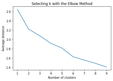
Then I have randomly split data into train and test splits (70/30) to train and test my k-means model. In order to test influence of cluster number and select the best number of clusters, I have conducted series of analysis, fitting model with k=1-9 clusters. The variance in the clustering variables that was accounted for by the clusters (r-square) was plotted for each of the nine cluster solutions in an elbow curve to provide guidance for choosing the number of clusters to interpret. Results can be observed below:

Results for k=2,4 and 7can be interpreted due to the presence of a fracture point in this positions. I’ve selected k=4 for my further analysis

To reduce number of variables PCA analysis were performed.

A scatterplot of the first two canonical variables by cluster (Figure 2 shown below) can be seen below:

Cluster with green dots has low cluster variance somewhat, cluster with purple dots is also packed well enough, with some variance exists.

cluster with yellow dots isn't well separated from purple and Somewhat from cluster with purple , but it is much more spread on the plot

cluster with yellow it is much more spread on the plot, showing high variance in the plot. data is well separated (clusters overlap is not significant) k=>4 is a suitable number for current situation.

Cluster 0, had the highest Likelihood to be affected by Baseline value.

Cluster 3, includes fetals with higher likelihood of affected by Uterine contractions, Light decelerations, Severe decelerations,,Prolongued decelerations, Abnormal short term variability., Mean value of short term variability, Histogram mode

compared to the other two clusters. It also has higher levels affected by Histogram mean, Histogram median, Histogram variance.

In order to validate the clusters, ANOVA analysis was conducted to test for significant differences between the clusters on fetal health. Results indicated significant differences between the clusters on GPA (F(2, 1485)= 420.2, p<.0001). The tukey test showed that clusters differ significantly within fetal health, although difference between cluster 2 and 3 is not significant.

CODE:

!pip install statsmodels

from pandas import Series, DataFrame

import pandas as pd

import numpy as np

import matplotlib.pylab as plt

from sklearn.model_selection import train_test_split

from sklearn import preprocessing

from sklearn.cluster import KMeans

from scipy.spatial.distance import cdist

from sklearn.decomposition import PCA

import statsmodels.formula.api as smf

import statsmodels.stats.multicomp as multi

%matplotlib inline

RND_STATE = 2226

!pip install pandas

!pip install numpy

!pip install matplotlib

!pip install statsmodels

data = pd.read_csv("fetal_health.csv")

data.columns = map(str.upper, data.columns)

data_clean = data.dropna()

AH_data = pd.read_csv("fetal_health.csv")

data_clean = AH_data.dropna()

cluster=data_clean[['baseline value','uterine_contractions','light_decelerations','severe_decelerations',

'prolongued_decelerations',

'abnormal_short_term_variability','mean_value_of_short_term_variability',

'histogram_mode','histogram_mean',

'histogram_median','histogram_variance']]

cluster.describe()

clustervar=cluster.copy()

clustervar['baseline value']=preprocessing.scale(clustervar['baseline value'].astype('float64'))

clustervar['uterine_contractions']=preprocessing.scale(clustervar['uterine_contractions'].astype('float64'))

clustervar['light_decelerations']=preprocessing.scale(clustervar['light_decelerations'].astype('float64'))

clustervar['severe_decelerations']=preprocessing.scale(clustervar['severe_decelerations'].astype('float64'))

clustervar['prolongued_decelerations']=preprocessing.scale(clustervar['prolongued_decelerations'].astype('float64'))

clustervar['abnormal_short_term_variability']=preprocessing.scale(clustervar['abnormal_short_term_variability'].astype('float64'))

clustervar['mean_value_of_short_term_variability']=preprocessing.scale(clustervar['mean_value_of_short_term_variability'].astype('float64'))

clustervar['histogram_mode']=preprocessing.scale(clustervar['histogram_mode'].astype('float64'))

clustervar['histogram_mean']=preprocessing.scale(clustervar['histogram_mean'].astype('float64'))

clustervar['histogram_median']=preprocessing.scale(clustervar['histogram_median'].astype('float64'))

clustervar['histogram_variance']=preprocessing.scale(clustervar['histogram_variance'].astype('float64'))

clus_train, clus_test = train_test_split(clustervar, test_size=0.3, random_state=RND_STATE)

!pip install cluster

clusters=range(1,10)

meandist=[]

for k in clusters:

model=KMeans(n_clusters=k)

model.fit(clus_train)

clusassign=model.predict(clus_train)

meandist.append(sum(np.min(cdist(clus_train, model.cluster_centers_, 'euclidean'), axis=1))

/ clus_train.shape[0])

!pip install statsmodels

!pip install matplotlib

!pip install scipy

plt.plot(clusters, meandist)

plt.xlabel('Number of clusters')

plt.ylabel('Average distance')

plt.title('Selecting k with the Elbow Method')

plt.show()

model3=KMeans(n_clusters=3)

model3.fit(clus_train)

clusassign=model3.predict(clus_train)

pca_2 = PCA(2)

plot_columns = pca_2.fit_transform(clus_train)

plt.scatter(x=plot_columns[:,0], y=plot_columns[:,1], c=model3.labels_,)

plt.xlabel('Canonical variable 1')

plt.ylabel('Canonical variable 2')

plt.title('Scatterplot of Canonical Variables for 3 Clusters')

plt.show()

clus_train.reset_index(level=0, inplace=True)

cluslist=list(clus_train['index'])

labels=list(model3.labels_)

newlist=dict(zip(cluslist, labels))

newclus=DataFrame.from_dict(newlist, orient='index')

newclus.columns = ['cluster']

newclus.describe()

newclus.reset_index(level=0, inplace=True)

merged_train=pd.merge(clus_train, newclus, on='index')

merged_train.head(n=100)

merged_train.cluster.value_counts()

clustergrp = merged_train.groupby('cluster').mean()

print ("Clustering variable means by cluster")

print(clustergrp)

gpa_data=data_clean['fetal_health']

gpa_train, gpa_test = train_test_split(gpa_data, test_size=.3, random_state=RND_STATE)

gpa_train1=pd.DataFrame(gpa_train)

gpa_train1.reset_index(level=0, inplace=True)

merged_train_all=pd.merge(gpa_train1, merged_train, on='index')

sub1 = merged_train_all[['fetal_health', 'cluster']].dropna()

gpamod = smf.ols(formula='fetal_health ~ C(cluster)', data=sub1).fit()

print (gpamod.summary())

print ('means for fetal health by cluster')

m1= sub1.groupby('cluster').mean()

print (m1)

print ('standard deviations for fetal health by cluster')

m2= sub1.groupby('cluster').std()

print (m2)

mc1 = multi.MultiComparison(sub1['fetal_health'], sub1['cluster'])

res1 = mc1.tukeyhsd()

print(res1.summary())

0 notes

natoli2001 · 4 years ago

Text

The elbow curve was inconclusive, suggesting that the 2, 4 and 8-cluster solutions might be interpreted. The results below are for an interpretation of the 4-cluster solution.

Canonical discriminant analyses was used to reduce the 11 clustering variable down a few variables that accounted for most of the variance in the clustering variables. A scatterplot of the first two canonical variables by cluster (Figure 2 shown below) indicated that the observations in clusters 1 and 4 were densely packed with relatively low within cluster variance, and did not overlap very much with the other clusters. Cluster 2 was generally distinct, but the observations had greater spread suggesting higher within cluster variance. Observations in cluster 3 were spread out more than the other clusters, showing high within cluster variance. The results of this plot suggest that the best cluster solution may have fewer than 4 clusters, so it will be especially important to also evaluate the cluster solutions with fewer than 4 clusters.

Figure 2. Plot of the first two canonical variables for the clustering variables by cluster.

0 notes

data-analytical · 4 years ago

Text

K-Means Cluster Analysis

I really didn't enjoy this assignment. It is so involved and there's so little data in my dataset, it is not a terribly good example of the method in action. Also, the sample script doesn't work out of the box, so it was hard initially, to run and compare. Here goes...

I ran a K-Means Cluster Analysis to look at underlying sub-groups of countries based on their similar responses through the following variables:

polityscore

incomeperperson

alcconsumption

breastcancerper100th

co2emissions

employrate

internetuserate

oilperperson

relectricperperson

suicideper100th

urbanrate

All clustering variables were standardized to have a mean of 0 and a standard deviation of 1.

I did NOT use the SurveySelect Procedure, to split out test/training data, because my initial dataset is only 56 rows (after missing data deletion).

A series of k-means cluster analyses were conducted on the training data specifying k=1-9 clusters, using Euclidean distance. The variance in the clustering variables that was accounted for by the clusters (r-square) was plotted for each of the nine cluster solutions in an elbow curve to provide guidance for choosing the number of clusters to interpret.

Figure 1. Elbow curve of r-square values for the nine cluster solutions.

The elbow curve was very inconclusive, suggesting that the 2, 3, 5 and 6-cluster solutions might be interpreted. Keeping in mind that I have very little data to cluster (so I cannot be certain about anything), I opted to investigate the 3-cluster solution.

I ran Canonical Discriminant Analysis reducing my 11 variables to a more manageable number.

Figure 2. Plot of the first two canonical variables for the clustering variables by cluster. Means procedure.

The lack of data reveals itself in the chart. Cluster 2 only appears to have contained only 2 data points! However, clusters 1 and 3 did show a degree of clustering. Cluster 1 was more densely packed than 3, but clearly, both displayed variance within themselves. Both clusters appeared to be distinct. That said, results could be very different, if I had more data to work with!

Because low amount of observations, I feel that a two cluster analysis would be the most effective in this case. However, because cluster 2 has almost no data within it, I am forced to use 3.

The Clustering Means Analysis on the 3 cluster solution shows the following highlights:

Cluster1

Very low (negative) levels of income, alcoholconsumptionm breastcancer, internetusage, oilperperson, retailelectricperperson and urbanization.

Very high levels of employment.

Cluster2

Omitted - because of the low amount of data in the cluster

Cluster3

Very low (negative) levels of income, alcoholconsumptionm breastcancer, internetusage, oilperperson, retailelectricperperson and urbanization.

Very high levels of incomepeperson, breastcancerper100th, co2 emission, electricity.

Moderate to low levels of political score, alcoholconsumption and suicide.

Figure 3. Means Chart.

Whilst, once again it would be dangerous to draw too many conclusions from such a low dataset, Cluster 3 seems to be a little more comparable to a developed country, perhaps with better medical care (or access to it), which might extend the average persons life.

In order to externally validate the clusters, an Analysis of Variance (ANOVA) was conducting to test for significant differences between the clusters on lifeexpectancy.

Figure 4. ANOVA Chart and tables.

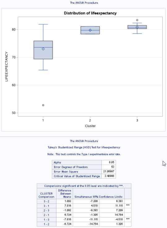
I used a tukey test used for post hoc comparisons between the clusters. Results indicated significant differences between the clusters on lifeexpectancy (F(2, 53)=17.21, p<.0001).

Countries in cluster 3 had the highest lifeexpectancy (mean=2.36, sd=0.78), and cluster 1 had the lowest (mean=2.67, sd=0.76).

Here is the code that I used to produce this analysis...

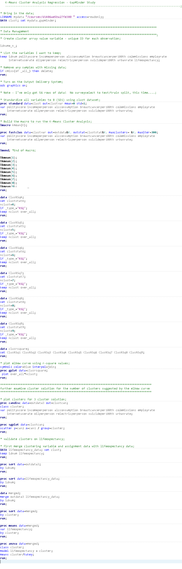
If I had more data, I could probably use this model with more confidence. Because the model tends to expect uniform and more sizable clusters of data (and my data clearly was not), I would be unhappy making any major decisions, based upon this analysis.

0 notes