#properties of inverse trigonometric functions

[inversetrigonometricfunctions]

Class 12 Maths Inverse Trigonometric Functions Course | JEE Mains की तैयारी | MathYug

अगर आप Class 12 Maths में Inverse Trigonometric Functions अच्छे से समझना चाहते हैं और साथ ही JEE Mains की भी तैयारी कर रहे हैं, तो MathYug का यह कोर्स आपके लिए बहुत फायदेमंद है। इस कोर्स में expert teacher Ashish Sir ने हर concept को आसान भाषा में समझाया है।

आप इस course में सीखेंगे:

Inverse Trigonometric Functions की definition

Domain और range

Principal value branches

Graphs और identities

Elementary properties

सिर्फ समझना ही नहीं, बल्कि concept को और पक्का करने के लिए NCERT textbook, exemplar, RD Sharma और Board’s Question Bank से चुने गए questions को assignments के तौर पर दिया गया है। इन assignments की PDF भी download की जा सकती है।

यह कोर्स Class 12 students के साथ-साथ JEE Mains aspirants के लिए भी designed है, ताकि दोनों ही exams की तैयारी एक साथ हो सके।

MathYug आपको expert guidance, professional notes, और structured learning के साथ एक complete learning experience देता है। Join कीजिए और अपने maths concepts को strong बनाइए।

Join the complete course now at: https://mathyug.com/c/ch2-inverse-trigonometric-functions/

[sethiswiftlearn]

Class 12 Math | Inverse Trigonometric functions | CBSE and State boards | JEE Mains, CUET Prep

Master Inverse Trigonometric Functions with this in-depth session designed for Class 12 CBSE, State Boards, JEE Mains, and CUET preparation. Learn essential concepts, formulas, and problem-solving techniques to boost your understanding and exam performance. This video includes step-by-step explanations and previous year questions (PYQs) for thorough practice.

📌 Key Takeaways: ✔️ Concept clarity on inverse trigonometric functions ✔️ Important formulas and properties ✔️ Solved examples and PYQs ✔️ Perfect for CBSE, State Boards, JEE Mains & CUET

📺 Watch now: https://youtu.be/QuiZLqiBp94?si=cd-osoS7xPUIwQJF

🔔 Subscribe for more math lessons and exam tips!

[subhasapco123]

Understanding Inverse Trigonometric Functions: A Comprehensive Guide

Trigonometry is one of the foundational subjects in mathematics that finds applications in various fields such as physics, engineering, and even computer science. While trigonometric functions like sine, cosine, and tangent describe relationships between the sides and angles of a right triangle, inverse trigonometric functions are equally essential for solving problems that involve angles when the sides of the triangle are known.

Inverse trigonometric functions, as the name suggests, are the reverse of the standard trigonometric functions. This blog will explore the concept of inverse trigonometric functions, their properties, and how they are used in mathematical and real-world applications.

What are Inverse Trigonometric Functions?

The inverse trigonometric functions are the functions that reverse the action of the regular trigonometric functions. In simple terms, while a regular trigonometric function takes an angle and gives a ratio of sides (such as sine giving opposite/hypotenuse), an inverse trigonometric function takes a ratio and gives an angle.

The six trigonometric functions in mathematics are:

Sine (sin)

Cosine (cos)

Tangent (tan)

Cotangent (cot)

Secant (sec)

Cosecant (csc)

Each of these functions has an associated inverse function. For example, the inverse of sine is called arcsine (or sin⁻¹), the inverse of cosine is called arccosine (cos⁻¹), and so on.

Why Do We Need Inverse Trigonometric Functions?

Inverse trigonometric functions are crucial because they allow us to find the angle when we know the value of the trigonometric function. This is particularly useful in fields like navigation, physics, engineering, and computer graphics, where it’s essential to work backward from a ratio of sides to determine the angle.

For instance, if we know the sine of an angle in a right triangle, the inverse sine (sin⁻¹) function can help us determine the measure of the angle. Similarly, inverse functions like arctangent (tan⁻¹) help us find the angle when the ratio of the opposite side to the adjacent side is known.

The Notation of Inverse Trigonometric Functions

The notation for inverse trigonometric functions is a bit different from regular trigonometric functions. Instead of writing "sin(x)" or "cos(x)," the inverse trigonometric functions are denoted with a superscript minus one, such as sin⁻¹(x) or cos⁻¹(x). This notation represents the angle whose sine or cosine is the given value.

Here’s a quick list of the common inverse trigonometric functions:

sin⁻¹(x) or arcsin(x): The inverse of sine, gives the angle whose sine is x.

cos⁻¹(x) or arccos(x): The inverse of cosine, gives the angle whose cosine is x.

tan⁻¹(x) or arctan(x): The inverse of tangent, gives the angle whose tangent is x.

cot⁻¹(x) or arccot(x): The inverse of cotangent, gives the angle whose cotangent is x.

sec⁻¹(x) or arcsec(x): The inverse of secant, gives the angle whose secant is x.

csc⁻¹(x) or arccsc(x): The inverse of cosecant, gives the angle whose cosecant is x.

Domains and Ranges of Inverse Trigonometric Functions

One of the critical aspects of inverse trigonometric functions is that they are restricted to certain domains and ranges to ensure that they are one-to-one functions. A one-to-one function is essential because it ensures that each input corresponds to a unique output.

Arcsin (sin⁻¹):

Domain: -1 ≤ x ≤ 1

Range: -π/2 ≤ y ≤ π/2

The arcsin function gives an angle between -90° and 90°.

Arccos (cos⁻¹):

Domain: -1 ≤ x ≤ 1

Range: 0 ≤ y ≤ π

The arccos function gives an angle between 0° and 180°.

Arctan (tan⁻¹):

Domain: -∞ < x < ∞

Range: -π/2 < y < π/2

The arctan function gives an angle between -90° and 90°.

Arccot (cot⁻¹):

Domain: -∞ < x < ∞

Range: 0 < y < π

The arccot function gives an angle between 0° and 180°.

Arcsec (sec⁻¹):

Domain: |x| ≥ 1

Range: 0 ≤ y ≤ π/2 or π ≤ y ≤ 3π/2

The arcsec function gives an angle between 0° and 90° or between 90° and 180°.

Arccsc (csc⁻¹):

Domain: |x| ≥ 1

Range: -π/2 ≤ y ≤ 0 or 0 ≤ y ≤ π/2

The arccsc function gives an angle between -90° and 90°, excluding 0°.

Properties of Inverse Trigonometric Functions

Understanding the properties of inverse trigonometric functions can make working with them much easier. Here are some essential properties:

Inverse of an Inverse: The inverse of an inverse trigonometric function gives the original function back. For example:

sin(sin⁻¹(x)) = x for -1 ≤ x ≤ 1

cos(cos⁻¹(x)) = x for -1 ≤ x ≤ 1

tan(tan⁻¹(x)) = x for all x

Composition of Functions: The inverse and the original trigonometric function can be composed together. For example:

sin⁻¹(sin(x)) = x for -π/2 ≤ x ≤ π/2

cos⁻¹(cos(x)) = x for 0 ≤ x ≤ π

tan⁻¹(tan(x)) = x for -π/2 < x < π/2

Symmetry: Inverse trigonometric functions exhibit symmetry about certain axes. For example, the inverse sine function is symmetric about the y-axis, while the inverse cosine function is symmetric about the line x = 0.

Solving Trigonometric Equations Using Inverse Functions

Inverse trigonometric functions are widely used for solving trigonometric equations. For example, if you are given a problem where you need to find the angle θ, knowing the value of sin(θ) = 0.5, you can use the arcsin function to find the angle:θ=sin⁡−1(0.5)=30∘�� = \sin^{-1}(0.5) = 30^\circθ=sin−1(0.5)=30∘

Similarly, if you are given the tangent value of an angle, you can use the arctan function to find the angle. This process is vital for solving problems in geometry, calculus, and physics.

Real-World Applications of Inverse Trigonometric Functions

Navigation: Inverse trigonometric functions are crucial in navigation and determining bearings. Pilots and sailors use these functions to calculate angles based on given distances and directions.

Physics: In physics, especially in wave motion and optics, inverse trigonometric functions help solve problems involving angles of refraction, angles of incidence, and angular displacement.

Engineering: In electrical engineering and mechanical systems, inverse trigonometric functions are used in control systems, signal processing, and analyzing vibrations.

Computer Graphics: Inverse trigonometric functions are used in computer graphics to rotate and scale objects, especially when working with angles in 3D space.

Conclusion

Inverse trigonometric functions are indispensable tools for solving mathematical and real-world problems involving angles and ratios. From geometry to physics and engineering, they provide a method for determining the angle when the side ratios of a right triangle are known. Understanding the properties and applications of inverse trigonometric functions will undoubtedly help you excel in both theoretical and applied mathematics.

[cbse-board]

Detailed explanation of ‘how to drive identities of Inverse Trigonometric Functions and questions based on NCERT Solutions for Inverse Trigonometric Functions Class 12 Maths Chapter 2.

#InverseTrigonometricFunctions #Class12Maths

[ashishkumarletslearn]

Full Syllabus of Class 12 Maths 

Ch01. Relations and Functions (Part – 1) Ch01. Relations and Functions (Part – 2) Ch02. Inverse Trigonometric Functions Ch03. Matrices Class 12 Maths Ch03. Matrices Class 12 Assignments Ch04. Determinants Class 12 Maths Ch04. Determinants Class 12 Assignments Ch05. Continuity and Differentiability Class 12 Maths Ch05. Continuity and Differentiability (Derivative Assignments) Class 12 Assignments Ch05. Continuity and Differentiability (Differentiability Assignment – 3) Class 12 Assignments Ch06. Applications of Derivatives Ch06. Applications of Derivatives Class 12 Assignments Ch07. Integrals Ch07. Properties of Integrals Ch08. Limit of Sum & Application of Definite Integrals Ch09. Differential Equations Ch10. Vector Algebra Class 12 Maths Ch10. Vector Algebra Class 12 Assignments Ch11. Three Dimensional Geometry Class 12 Maths Ch12. Linear Programming Problems Ch13. Probability

[ancientmariner13]

Properties of Inverse Trigonometric Functions

Another day, another new thing learnt! Thank God and my teacher that I understood well. I hope I am able to apply these to the upcoming problems as well. ❤️

🎧- Wonderland (Taylor Swift)

[topchildadoptionguide]

How to solve for y

Solving for 'y' is a fundamental skill in mathematics that is often encountered in algebraic equations and functions. Whether you're a student learning the basics or an adult refreshing your math skills, understanding how to solve for 'y' opens the door to a deeper comprehension of equations and their solutions. In this article, we will provide you with a step-by-step guide on how to solve for 'y' in various scenarios, equipping you with the tools to tackle equations with confidence.

Understand the Equation Type: Before diving into solving for 'y', it's crucial to identify the type of equation you're working with. Equations can be linear, quadratic, exponential, logarithmic, or trigonometric, among others. Each equation type requires specific techniques and strategies for solving. Familiarize yourself with the characteristics of the equation at hand to determine the appropriate approach.

Isolate 'y' on One Side: The goal is to isolate the variable 'y' on one side of the equation. To achieve this, use algebraic operations such as addition, subtraction, multiplication, and division to move terms and constants from one side of the equation to the other. Perform the same operation on both sides to maintain equality. Continue simplifying the equation until 'y' is isolated.

Solve Linear Equations: In linear equations, 'y' typically appears as a coefficient multiplied by 'x' or other variables. To solve for 'y', isolate the term containing 'y' on one side of the equation by applying inverse operations. For example, if 'y' is multiplied by a coefficient, divide both sides of the equation by that coefficient. Simplify further until 'y' is isolated.

Solve Quadratic Equations: Quadratic equations involve 'y' raised to the power of 2. To solve for 'y', rearrange the equation into the standard quadratic form (ax^2 + bx + c = 0). Utilize factoring, completing the square, or the quadratic formula to find the values of 'y'. Be mindful of possible solutions, including real and complex numbers.

Solve Exponential and Logarithmic Equations: Exponential and logarithmic equations involve 'y' as the exponent or argument. To solve for 'y', use logarithmic properties to transform the equation into a manageable form. Apply inverse operations, such as exponentiation or taking the logarithm, to isolate 'y' and find its value.

Solve Trigonometric Equations: Trigonometric equations involve 'y' as part of a trigonometric function (sin, cos, tan, etc.). To solve for 'y', apply trigonometric identities and properties to simplify the equation. Utilize inverse trigonometric functions or trigonometric identities to isolate 'y' and determine its value. Pay attention to the specific domain restrictions and periodicity of trigonometric functions.

Check Your Solution: After obtaining a value for 'y', it's crucial to check your solution by substituting it back into the original equation. Ensure that the equation holds true when 'y' is replaced with the determined value. This step confirms the accuracy of your solution and verifies that you haven't made any calculation errors.

Solving for 'y' is an essential skill in mathematics that allows you to find solutions to various types of equations. By understanding the equation type, isolating 'y', and employing appropriate techniques for linear, quadratic, exponential, logarithmic, and trigonometric equations, you can confidently find the value of 'y'. Regular practice and familiarity with algebraic operations will strengthen your ability to solve equations and deepen your mathematical understanding. Embrace the challenge, apply the techniques, and enjoy the satisfaction of successfully solving for 'y' in any equation that comes your way.

[mathsprogram]

Get critical topics cover like algebra, geometry, trigonometry

Most students find the critical topics in high school mathematics as algebra, geometry, trigonometry, and calculus. These topics can be difficult for some students, but most students can succeed with a little extra help and practice. Various resources are available to help students, including online tools, textbooks, and teacher assistance.

What critical topics in algebra should students be aware of?

Algebra is a subject of interest that all learners have to master. It lays the groundwork for more advanced mathematics courses, and is essential for students who want to pursue a career in mathematics or science. So one must definitely enroll for best math tutoring in Dubai. Students should be aware of a few key topics before taking any algebra course. First, algebra is all about solving equations. To succeed in algebra, students need to be able to comprehend and solve equations of all kinds. Second, algebra also involves resolving equational systems. Students must be able to recognise and graph the solution set in order to solve an equation system. Finally, algebra is also about manipulating algebraic expressions. Students need to be able to rewrite expressions in order to make them easier to work with. Students who understand these key topics will be well prepared for an algebra course. 

 There are a few basic skills that students need to be successful in algebra. First, students need to be able to solve equations. They should be able to understand and solve equations of all types, including linear, quadratic, and systems of equations. Second, students need to be able to graph linear equations. They should be able to identify the x and y-intercepts and the slope of a line. Finally, students need to be able to manipulate algebraic expressions. They should be able to rewrite expressions in order to make them easier to work with. If students can master these skills, they will be well prepared for an algebra course.

 What are some critical topics in geometry that students should be aware of?

In geometry, there are a few critical topics that students should be aware of in order to succeed in the course. These topics include angles, points, lines, and planes. To complete the other geometry concepts, these concepts are essential to understand. For example, in order to understand geometric proofs, students must first understand angles and how to measure them. Additionally, points, lines, and planes are used to construct geometric shapes. By understanding these critical topics, students can build a strong foundation in geometry and be better prepared for future mathematics courses. Angles are generated by intersecting two lines. The measure of an angle is determined by the size of the two lines that form the angle and the distance between the lines. The measure of an angle is always between 0 and 360 degrees. Points are locations in space that have no dimension. A dot on a piece of paper represents points. Lines are straight, infinite, infinitely thin objects that have no width. A set of two points represents lines. Planes are flat, two-dimensional objects that have width and length, but no depth. Planes are represented by a set of points that lie in the same plane.

What are some critical topics in trigonometry that students should be aware of?

One of the most important things students need to know in trigonometry is how to use the different trigonometric functions. These functions can be used to solve a variety of problems, so students need to understand how to use them. Additionally, students should be aware of the different properties of the trigonometric functions. For illustration, the sine and cosine functions are periodic, meaning that their values repeat repeatedly. Students should also understand the inverse functions of the trigonometric functions, which can be used to solve problems in reverse. Finally, students need to be familiar with the different types of triangles and how to use the trigonometric functions to find the angles and sides of these triangles. This can be done by seeking help from the online math tutor.

Reach out to Mathnasium's experts for sat math help in uae, learn math lessons in sharjah, and get help with math test prep in dubai.

[math-cheat-sheet-z8]

math cheat sheet 100% working U9F%

💾 ►►► DOWNLOAD FILE 🔥🔥🔥🔥🔥 Geometry- Circles, Arcs, and Diameters Cheat Sheet. this is a cheat sheet for the annoying circles and stuff. Here is list of cheat sheets and tables that I've written. With the exception of the Complete Calculus Cheat Sheet and the Integrals. High-school math cheat sheets, covering algebra, trigonometry, coordinate geometry and calculus. Downloadable as PDFs. Dec 9, - This post has been a long time in the making. It's a collection of free math cheat sheets that you can print and give to students for thei. 9 This section contains high school math cheat sheets covering algebra, trigonometry, coordinate geometry and calculus. Each cheat sheet covers the summary of concepts and the most important formulas related to the particular chapter in a single page. Currently there are 33 cheat sheets in total, with more to be added soon. Download them all! If you wish to give feedback, please send me a message on Facebook. For learning these concepts in detail, please visit the Lessons page. Also check out my YouTube channel for cool mathy stuff coming soon. Follow the Twitter account and like the Facebook page for updates on new lessons, cheat sheets, problems and random fun stuff. Home » Cheat Sheets. Area Under Curves. Complex Numbers. Conditional Identities. Coordinate Geometry. Definite Integrals. Differential Equations. Graph Transformations. Graph Transformations Advanced. Ceiling and Floor Functions. Indefinite Integrals. Inverse Trigonometric Functions. Inverse Trigonometric Functions Graphs. Mathematical Logic. Matrices [Coming Soon]. Properties of Triangles. Quadratic Equations. Set Theory. Straight Line. Solution of Triangles. Trigonometric Equations. Trigonometric Graphs. Trigonometric Identities. Trigonometric Ratios. Vector Algebra. Vector Geometry. Thanks for visiting!

[dcgexampreparation]

Indian Air Force Agniveer Syllabus 2022 and Exam Pattern

Agnipath is a new scheme introduced by the Govt. of India on June 14, 2022, for the recruitment of soldiers below the rank of commissioned officers into the three services (Indian Army, Indian Air Force, and Indian Navy) of the armed forces. Soldiers recruited under this scheme will be recognized as ‘Agniveers’. 

The Indian Air Force has released the official notification for the recruitment of Agniveers under the Agnipath scheme. The online application process for the recruitment of the Indian Air Force Agniveer Vayu has started from 24th June,2022. The interested and eligible candidate can directly apply from the official website of the Indian Air Force. The Indian Air Force Agniveer will be recruited on the basis of a written exam, a physical fitness test, a physical measurement test, and a medical test.

Indian Air Force Exam Pattern 2022

The detailed exam pattern for the Air Force Agniveer Recruitment 2022 is mentioned below :

Science Subjects:- The total duration of the online test shall be 60 minutes and shall comprise English, Physics, and Mathematics as per the 10+2 CBSE syllabus.

Other Than Science Subjects:- The total duration of the online test shall be 45 minutes and shall comprise English as per the 10+2 CBSE syllabus and Reasoning & General Awareness.

Science Subjects & Other Than Science Subjects:- The total duration of the online test shall be 85 minutes and shall comprise English, Physics, and Mathematics as per the 10+2 CBSE syllabus and Reasoning & General Awareness (RAGA).

 The Marking Pattern for the online tests:

One Mark for Every Correct Answer.

Nill(0)  marks for unattempted questions.

There will be negative marking & 0.25 marks will be deducted from each wrong answer

To ease your preparation, DCG Defence Academy in Pune has launched the Agniveer Vayu complete batch along with both online and offline modes to check your performance on a daily basis. DCG Defence Academy is one of the best Indian Air Force Agniveer Coaching Academy in Pune and provides the best air force exam classes.

Indian Air Force Agniveer Syllabus 2022

In the written exam, questions will  be asked from the subjects such as General Knowledge and reasoning, Maths , Physics, and Chemistry. The mode of the Indian Air Force Exam is online and the duration of the exam differs for different groups. The detailed syllabus for different subjects in the Indian Air Force Agniveer written exam is mentioned below:

Abbreviations

Science – Inventions & Discoveries

Current Important Events

Current Affairs – National & International

Awards and Honours

Indian Constitution

Books and Authors

Important Days

History

Sports Terminology

Geography

Solar System

Indian States and Capitals

Countries and Currencies

Indian Air Force Syllabus For Mathematics

Mixture & Allegations

Pipes and Cisterns

Speed, Time & Distance (Train, Boats & Stream)

Mensuration

Trigonometry

Geometry

Time and Work

Probability

HCF & LCM

Algebraic Expressions and inequalities

Average

Percentage

Profit and Loss

Number System

Speed, Distance, and Time

Simple & Compound interest

Ratio and Proportion

Partnership

Data Interpretation

Number Series

Indian Air Force Agniveer Syllabus for Science

Laws of motion

Communication System

Trigonometric & Inverse Trigonometric functions

Sets, relations, and functions

Electronic devices

Optics

Sequence and series

Kinematics

Waves and Oscillations

Physical-world and measurement

The behaviour of perfect gases and the kinetic theory of gases & Atoms and Nuclei

Bulk matter properties

Magnetism and Magnetic effects of current

Radiation and Dual nature of matter

Electromagnetic Waves

Straight lines and family of lines

Vector

Work, Power, and Energy

Electromagnetic induction and Alternating current

Electrostatics & Current Electricity

The motion of a system of particles and rigid body

Thermodynamics

Gravitation & Statistics

Laws of motion

Communication System

Trigonometric & Inverse Trigonometric functions

Sets, relations, and functions

Electronic devices

Optics

Sequence and series

Kinematics

Waves and Oscillations

Physical-world and measurement

The behaviour of perfect gases and the kinetic theory of gases & Atoms and Nuclei

Bulk matter properties

Magnetism and Magnetic effects of current

Radiation and Dual nature of matter

Electromagnetic Waves

Straight lines and family of lines

Vector

Work, Power, and Energy

Electromagnetic induction and Alternating current

Electrostatics & Current Electricity

The motion of a system of particles and rigid body

Thermodynamics

Gravitation & Statistics

DCG Defence Academy provides the best Air Force Agniveer Coaching Classes in Pune with the best faculties that prepare the students well for Agniveer training physically as well as mentally. It also conducted seminars, webinars, and extra doubt classes for the students. DCG Defence Academy is well known for its academic performance that imparts coaching and guidance to young and dynamic aspirants and moulds them into successful officers in defence serving the nation.

[sethiswiftlearn]

Class 12 Math | Mastering Inverse Trigonometric Functions | JEE Mains, CUET Preparation

Inverse Trigonometric Functions play a crucial role in Class 12 Mathematics, forming the foundation for calculus and higher-level mathematics. A strong grasp of these concepts is essential for excelling in JEE Mains, CUET, and other competitive exams. This session is designed to help students master the properties, domain, range, and applications of inverse trigonometric functions with easy explanations and problem-solving techniques.

What You’ll Learn in This Session?

✔ Definition & Basic Concepts – Understanding inverse trigonometric functions and their significance. ✔ Domain and Range – A clear breakdown of how to determine valid input values. ✔ Principal Branches & Graphs – How to visualize and interpret inverse trigonometric functions. ✔ Important Identities & Formulas – Mastering standard formulas for solving complex problems. ✔ Differentiation & Integration of Inverse Trigonometric Functions – A critical aspect for calculus-based questions. ✔ Exam-Focused Problem Solving – Previous year JEE Mains, CUET, and CBSE Board questions with step-by-step solutions.

Why Watch This Session?

Boost Conceptual Understanding – Strengthen your fundamentals for competitive exams.

Solve Problems Faster – Learn shortcuts and tricks to tackle tricky questions easily.

High-Weightage Topic – This topic frequently appears in JEE Mains, CUET, and Board exams.

Step-by-Step Explanations – Detailed solutions to help you gain confidence in solving problems.

📌 Watch Now & Ace Your Math Exams! 👉 https://youtu.be/Y1o0AlflWsI?si=A-VnLoDg6vNwlUrl

🔔 Subscribe for More! Stay tuned for more revision sessions, exam tricks, and concept explanations to help you master Class 12 Mathematics. 🚀

[acemywriter]

Calculus Question

Trig/Calc live assignment tomorrow at 12 PM EST. Topics include properties of real number system, inequalities, theory or equations, complex numbers, the study of functions including inverse functions, logarithmic and exponential functions, trigonometric functions with emphasis on circular functions, trigonometric identities, trigonometric equations, graphical methods and solving triangles with…

[foxspain82]

10.4 Usubstitution Trig Functionsap Calculus

10.4 U-substitution Trig Functionsap Calculus Answers

10.4 U-substitution Trig Functionsap Calculus Pdf

10.4 U-substitution Trig Functionsap Calculus Problems

10.4 U-substitution Trig Functionsap Calculus Worksheet

Calculus II, Section 7.4, #67 Integration of Rational Functions by Partial Fractions One method of slowing the growth of an insect population without the use of pesticides is to introduce into the population a number of sterile males that mate with fertile females but produce no o spring. Let P represeent. AP Calculus AB Mu Alpha Theta Welcome to AP Calculus AB! Contact me here. Need more review? Browse the Algebra II and Pre-Calculus Tabs. AP ® Calculus AB and BC. COURSE AND EXAM DESCRIPTION. AP COURSE AND EXAM DESCRIPTIONS ARE UPDATED PERIODICALLY. Please visit AP Central. Mathematics 104—Calculus, Part I (4h, 1 CU) Course Description: Brief review of High School Calculus, methods and applications of integration, infinite series, Taylor's theorem, first order ordinary differential equations. Use of symbolic manipulation and graphics software in Calculus. Note: This course uses Maple®.

Math 104: Calculus I – Notes

Section 004 - Spring 2014

10.4 U-substitution Trig Functionsap Calculus Answers

Syllabus

Concept Videos

Skeleton NotesComplete Notes Title More Remainder 10.6, 10.9 Remainder 10.6/10.9 Series Estimation & Remainder Sections 10.8-10.10 Sections 10.8-10.10 Taylor (and Maclaurin) Series Section 10.7 Section 10.7 Power Series Introduction Section 10.6 Section 10.6 Alt. Series Test and Abs. Conv. Conv. Tests Section 10.5 Section 10.5 The Ratio and Root Tests Section 10.4 Section 10.4 The Comparison Tests Section 10.3 Section 10.3 The Integral Test Section 10.2 Section 10.2 Introduction to Series Section 10.1 Section 10.1 Sequences Section 9.2 Section 9.2 Linear Differential Equations Section 7.2 Pt 1Pt 2 Section 7.2 Separable Differential Equations Section 8.8 Section 8.8 Probability and Calculus Odd Ans. Section 8.7 Pt. 1Pt. 2Section 8.7 Improper Integrals L'Hopital Section 8.4 Pt. 1Pt. 2Section 8.4 Partial Fraction Decomposition Section 8.3 Pt. 1Pt. 2Section 8.3 Trig. Substitution Section 8.2 Pt. 1Pt. 2Section 8.2 Integrating Trig. Powers Section 8.1 Pt. 1Pt. 2 Section 8.1 Integration By Parts Section 6.6 Section 6.6 Center of Mass Section 6.4 Section 6.4 Surface Area of Revolution Section 6.3 Section 6.3 Arc Length Section 6.2Section 6.2 Volumes Using Cylindrical Shells Section 6.1 Section 6.1 Volumes Using Cross-Sections disk/washer Review Calc I Review Calc I ReviewLimit, Derivative, and Integral Area b/w CurvesArea b/w Curves Video Example U-substitution Graphs you should know

Print out the skeleton notes before class and bring them to class so that you don't have to write down https://foxspain82.tumblr.com/post/657282647494672384/achievement-unlocked-2watermelon-gaming. Hide paragraph marks in microsoft word for mac. everything said in class. If you miss anything, the complete notes will be posted after class.

10.4 U-substitution Trig Functionsap Calculus Pdf

My Penn Page | Penn Math 104 Page| Penn Undergraduate Math | Advice | Help|

10.4 U-substitution Trig Functionsap Calculus Problems

10.4 U-substitution Trig Functionsap Calculus Worksheet

Version #1 ​The course below follows CollegeBoard's Course and Exam Description. Lessons will begin to appear starting summer 2020. BC Topics are listed, but there will be no lessons available for SY 2020-2021

Unit 0 - Calc Prerequisites (Summer Work) 0.1 Summer Packet

Unit 1 - Limits and Continuity 1.1 Can Change Occur at an Instant? 1.2 Defining Limits and Using Limit Notation 1.3 Estimating Limit Values from Graphs 1.4 Estimating Limit Values from Tables 1.5 Determining Limits Using Algebraic Properties (1.5 includes piecewise functions involving limits) 1.6 Determining Limits Using Algebraic Manipulation 1.7 Selecting Procedures for Determining Limits (1.7 includes rationalization, complex fractions, and absolute value) 1.8 Determining Limits Using the Squeeze Theorem 1.9 Connecting Multiple Representations of Limits Mid-Unit Review - Unit 1 1.10 Exploring Types of Discontinuities 1.11 Defining Continuity at a Point 1.12 Confirming Continuity Over an Interval 1.13 Removing Discontinuities 1.14 Infinite Limits and Vertical Asymptotes 1.15 Limits at Infinity and Horizontal Asymptotes 1.16 Intermediate Value Theorem (IVT) Review - Unit 1

Unit 2 - Differentiation: Definition and Fundamental Properties 2.1 Defining Average and Instantaneous Rate of Change at a Point 2.2 Defining the Derivative of a Function and Using Derivative Notation (2.2 includes equation of the tangent line) 2.3 Estimating Derivatives of a Function at a Point 2.4 Connecting Differentiability and Continuity 2.5 Applying the Power Rule 2.6 Derivative Rules: Constant, Sum, Difference, and Constant Multiple (2.6 includes horizontal tangent lines, equation of the normal line, and differentiability of piecewise) 2.7 Derivatives of cos(x), sin(x), e^x, and ln(x) 2.8 The Product Rule 2.9 The Quotient Rule 2.10 Derivatives of tan(x), cot(x), sec(x), and csc(x) Review - Unit 2

Unit 3 - Differentiation: Composite, Implicit, and Inverse Functions 3.1 The Chain Rule 3.2 Implicit Differentiation 3.3 Differentiating Inverse Functions 3.4 Differentiating Inverse Trigonometric Functions 3.5 Selecting Procedures for Calculating Derivatives 3.6 Calculating Higher-Order Derivatives Review - Unit 3

Unit 4 - Contextual Applications of Differentiation 4.1 Interpreting the Meaning of the Derivative in Context 4.2 Straight-Line Motion: Connecting Position, Velocity, and Acceleration 4.3 Rates of Change in Applied Contexts Other Than Motion 4.4 Introduction to Related Rates 4.5 Solving Related Rates Problems 4.6 Approximating Values of a Function Using Local Linearity and Linearization 4.7 Using L'Hopital's Rule for Determining Limits of Indeterminate Forms Review - Unit 4

Unit 5 - Analytical Applications of Differentiation 5.1 Using the Mean Value Theorem 5.2 Extreme Value Theorem, Global Versus Local Extrema, and Critical Points 5.3 Determining Intervals on Which a Function is Increasing or Decreasing 5.4 Using the First Derivative Test to Determine Relative Local Extrema 5.5 Using the Candidates Test to Determine Absolute (Global) Extrema 5.6 Determining Concavity of Functions over Their Domains 5.7 Using the Second Derivative Test to Determine Extrema Mid-Unit Review - Unit 5 5.8 Sketching Graphs of Functions and Their Derivatives 5.9 Connecting a Function, Its First Derivative, and Its Second Derivative (5.9 includes a revisit of particle motion and determining if a particle is speeding up/down.) 5.10 Introduction to Optimization Problems 5.11 Solving Optimization Problems 5.12 Exploring Behaviors of Implicit Relations Review - Unit 5

Unit 6 - Integration and Accumulation of Change 6.1 Exploring Accumulation of Change 6.2 Approximating Areas with Riemann Sums 6.3 Riemann Sums, Summation Notation, and Definite Integral Notation 6.4 The Fundamental Theorem of Calculus and Accumulation Functions 6.5 Interpreting the Behavior of Accumulation Functions ​ Involving Area Mid-Unit Review - Unit 6 6.6 Applying Properties of Definite Integrals 6.7 The Fundamental Theorem of Calculus and Definite Integrals 6.8 Finding Antiderivatives and Indefinite Integrals: Basic Rules and Notation 6.9 Integrating Using Substitution 6.10 Integrating Functions Using Long Division ​ and Completing the Square 6.11 Integrating Using Integration by Parts (BC topic) 6.12 Integrating Using Linear Partial Fractions (BC topic) 6.13 Evaluating Improper Integrals (BC topic) 6.14 Selecting Techniques for Antidifferentiation Review - Unit 6

Unit 7 - Differential Equations 7.1 Modeling Situations with Differential Equations 7.2 Verifying Solutions for Differential Equations 7.3 Sketching Slope Fields 7.4 Reasoning Using Slope Fields 7.5 Euler's Method (BC topic) 7.6 General Solutions Using Separation of Variables 7.7 Particular Solutions using Initial Conditions and Separation of Variables 7.8 Exponential Models with Differential Equations 7.9 Logistic Models with Differential Equations (BC topic) Review - Unit 7

Unit 8 - Applications of Integration 8.1 Average Value of a Function on an Interval 8.2 Position, Velocity, and Acceleration Using Integrals 8.3 Using Accumulation Functions and Definite Integrals in Applied Contexts 8.4 Area Between Curves (with respect to x) 8.5 Area Between Curves (with respect to y) 8.6 Area Between Curves - More than Two Intersections Mid-Unit Review - Unit 8 8.7 Cross Sections: Squares and Rectangles 8.8 Cross Sections: Triangles and Semicircles 8.9 Disc Method: Revolving Around the x- or y- Axis 8.10 Disc Method: Revolving Around Other Axes 8.11 Washer Method: Revolving Around the x- or y- Axis 8.12 Washer Method: Revolving Around Other Axes 8.13 The Arc Length of a Smooth, Planar Curve and Distance Traveled (BC topic) Review - Unit 8

Unit 9 - Parametric Equations, Polar Coordinates, and Vector-Valued Functions (BC topics) 9.1 Defining and Differentiating Parametric Equations 9.2 Second Derivatives of Parametric Equations 9.3 Arc Lengths of Curves (Parametric Equations) 9.4 Defining and Differentiating Vector-Valued Functions 9.5 Integrating Vector-Valued Functions 9.6 Solving Motion Problems Using Parametric and Vector-Valued Functions 9.7 Defining Polar Coordinates and Differentiating in Polar Form 9.8 Find the Area of a Polar Region or the Area Bounded by a Single Polar Curve 9.9 Finding the Area of the Region Bounded by Two Polar Curves Review - Unit 9

Unit 10 - Infinite Sequences and Series (BC topics) 10.1 Defining Convergent and Divergent Infinite Series 10.2 Working with Geometric Series 10.3 The nth Term Test for Divergence 10.4 Integral Test for Convergence 10.5 Harmonic Series and p-Series 10.6 Comparison Tests for Convergence 10.7 Alternating Series Test for Convergence 10.8 Ratio Test for Convergence 10.9 Determining Absolute or Conditional Convergence 10.10 Alternating Series Error Bound 10.11 Finding Taylor Polynomial Approximations of Functions 10.12 Lagrange Error Bound 10.13 Radius and Interval of Convergence of Power Series 10.14 Finding Taylor Maclaurin Series for a Function 10.15 Representing Functions as a Power Series Review - Unit 8

Version #2 ​The course below covers all topics for the AP Calculus AB exam, but was built for a 90-minute class that meets every other day. Lessons and packets are longer because they cover more material.

Unit 0 - Calc Prerequisites (Summer Work) 0.1 Things to Know for Calc 0.2 Summer Packet 0.3 Calculator Skillz

Unit 1 - Limits 1.1 Limits Graphically 1.2 Limits Analytically 1.3 Asymptotes 1.4 Continuity Review - Unit 1

Unit 2 - The Derivative 2.1 Average Rate of Change 2.2 Definition of the Derivative 2.3 Differentiability (Calculator Required) ​ Review - Unit 2

Unit 3 - Basic Differentiation 3.1 Power Rule 3.2 Product and Quotient Rules 3.3 Velocity and other Rates of Change 3.4 Chain Rule 3.5 Trig Derivatives Review - Unit 3

Unit 4 - More Deriviatvies 4.1 Derivatives of Exp. and Logs 4.2 Inverse Trig Derivatives 4.3 L'Hopital's Rule Review - Unit 4

Unit 5 - Curve Sketching 5.1 Extrema on an Interval 5.2 First Derivative Test 5.3 Second Derivative Test Review - Unit 5

Unit 6 - Implicit Differentiation 6.1 Implicit Differentiation 6.2 Related Rates 6.3 Optimization ​ Review - Unit 6

Unit 7 - Approximation Methods 7.1 Rectangular Approximation Method 7.2 Trapezoidal Approximation Method Review - Unit 7

Unit 8 - Integration 8.1 Definite Integral 8.2 Fundamental Theorem of Calculus (part 1) 8.3 Antiderivatives (and specific solutions) Review - Unit 8

Unit 9 - The 2nd Fundamental Theorem of Calculus 9.1 The 2nd FTC 9.2 Trig Integrals 9.3 Average Value (of a function) 9.4 Net Change Review - Unit 9

Unit 10 - More Integrals 10.1 Slope Fields 10.2 u-Substitution (indefinite integrals) 10.3 u-Substitution (definite integrals) 10.4 Separation of Variables Review - Unit 10

Unit 11 - Area and Volume 11.1 Area Between Two Curves 11.2 Volume - Disc Method 11.3 Volume - Washer Method ​ 11.4 Perpendicular Cross Sections Review - Unit 11

[suzanneshannon]

Using Absolute Value, Sign, Rounding and Modulo in CSS Today

For quite a while now, the CSS spec has included a lot of really useful mathematical functions, such as trigonometric functions (sin(), cos(), tan(), asin(), acos(), atan(), atan2()), exponential functions (pow(), exp(), sqrt(), log(), hypot()), sign-related functions (abs(), sign()) and stepped value functions (round(), mod(), rem()).

However, these are not yet implemented in any browser, so this article is going to show how, using CSS features we already have, we can compute the values that abs(), sign(), round() and mod() should return. And then we’ll see what cool things this allows us to build today.

A few of the things these functions allow us to make.

Note that none of these techniques were ever meant to work in browsers from back in the days when dinosaurs roamed the internet. Some of them even depend on the browser supporting the ability to register custom properties (using @property), which means they’re limited to Chromium for now.

The computed equivalents

--abs

We can get this by using the new CSS max() function, which is already implemented in the current versions of all major browsers.

Let’s say we have a custom property, --a. We don’t know whether this is positive or negative and we want to get its absolute value. We do this by picking the maximum between this value and its additive inverse:

--abs: max(var(--a), -1*var(--a));

If --a is positive, this means it’s greater than zero, and multiplying it with -1 gives us a negative number, which is always smaller than zero. That, in turn, is always smaller than the positive --a, so the result returned by max() is equal to var(--a).

If --a is negative, this means it’s smaller than zero, and that multiplying it by -1 gives us a positive number, which is always bigger than zero, which, in turn, is always bigger than the negative --a. So, the result returned by max() is equal to -1*var(--a).

--sign

This is something we can get using the previous section as the sign of a number is that number divided by its absolute value:

--abs: max(var(--a), -1*var(--a)); --sign: calc(var(--a)/var(--abs));

A very important thing to note here is that this only works if --a is unitless, as we cannot divide by a number with a unit inside calc().

Also, if --a is 0, this solution works only if we register --sign (this is only supported in Chromium browsers at this point) with an initial-value of 0:

@property --sign { syntax: '<integer>'; initial-value: 0; inherits: false /* or true depending on context */ }

This is because --a, being 0, also makes --abs compute to 0 — and dividing by 0 is invalid in CSS calc() — so we need to make sure --sign gets reset to 0 in this situation. Keep in mind that this does not happen if we simply set it to 0 in the CSS prior to setting it to the calc() value and we don’t register it:

--abs: max(var(--a), -1*var(--a)); --sign: 0; /* doesn't help */ --sign: calc(var(--a)/var(--abs));

In practice, I’ve also often used the following version for integers:

--sign: clamp(-1, var(--a), 1);

Here, we’re using a clamp() function. This takes three arguments: a minimum allowed value -1, a preferred value var(--a) and a maximum allowed value, 1. The value returned is the preferred value as long as it’s between the lower and upper bounds and the limit that gets exceeded otherwise.

If --a is a negative integer, this means it’s smaller or equal to -1, the lower bound (or the minimum allowed value) of our clamp() function, so the value returned is -1. If it’s a positive integer, this means it’s greater or equal to 1, the upper bound (or the maximum allowed value) of the clamp() function, so the value returned is 1. And finally, if --a is 0, it’s between the lower and upper limits, so the function returns its value (0 in this case).

This method has the advantage of being simpler without requiring Houdini support. That said, note that it only works for unitless values (comparing a length or an angle value with integers like ±1 is like comparing apples and oranges — it doesn’t work!) that are either exactly 0 or at least as big as 1 in absolute value. For a subunitary value, like -.05, our method above fails, as the value returned is -.05, not -1!

My first thought was that we can extend this technique to subunitary values by introducing a limit value that’s smaller than the smallest non-zero value we know --a can possibly take. For example, let’s say our limit is .000001 — this would allow us to correctly get -1 as the sign for -.05, and 1 as the sign for .0001!

--lim: .000001; --sign: clamp(-1*var(--lim), var(--a), var(--lim));

Temani Afif suggested a simpler version that would multiply --a by a very large number in order to produce a superunitary value.

--sign: clamp(-1, var(--a)*10000, 1);

I eventually settled on dividing --a by the limit value because it just feels a bit more intuitive to see what minimum non-zero value it won’t go below.

--lim: .000001; --sign: clamp(-1, var(--a)/var(--lim), 1);

--round (as well as --ceil and --floor)

This is one I was stuck on for a while until I got a clever suggestion for a similar problem from Christian Schaefer. Just like the case of the sign, this only works on unitless values and requires registering the --round variable as an <integer> so that we force rounding on whatever value we set it to:

@property --round { syntax: '<integer>'; initial-value: 0; inherits: false /* or true depending on context */ } .my-elem { --round: var(--a); }

By extension, we can get --floor and --ceil if we subtract or add .5:

@property --floor { syntax: '<integer>'; initial-value: 0; inherits: false /* or true depending on context */ } @property --ceil { syntax: '<integer>'; initial-value: 0; inherits: false /* or true depending on context */ } .my-elem { --floor: calc(var(--a) - .5); --ceil: calc(var(--a) + .5) }

--mod

This builds on the --floor technique in order to get an integer quotient, which then allows us to get the modulo value. This means that both our values must be unitless.

@property --floor { syntax: '<integer>'; initial-value: 0; inherits: false /* or true depending on context */ } .my-elem { --floor: calc(var(--a)/var(--b) - .5); --mod: calc(var(--a) - var(--b)*var(--floor)) }

Use cases

What sort of things can we do with the technique? Let’s take a good look at three use cases.

Effortless symmetry in staggered animations (and not only!)

While the absolute value can help us get symmetrical results for a lot of properties, animation-delay and transition-delay are the ones where I’ve been using it the most, so let’s see some examples of that!

We put --n items within a container, each of these items having an index --i. Both --n and --i are variables we pass to the CSS via style attributes.

- let n = 16; .wrap(style=`--n: ${n}`) - for(let i = 0; i < n; i++) .item(style=`--i: ${i}`)

This gives us the following compiled HTML:

<div class='wrap' style='--n: 16'> <div class='item' style='--i: 0'></div> <div class='item' style='--i: 1'></div> <!-- more such items --> </div>

We set a few styles such that the items are laid out in a row and are square with a non-zero edge length:

$r: 2.5vw; .wrap { display: flex; justify-content: space-evenly; } .item { padding: $r; }

The result so far.

Now we add two sets of keyframes to animate a scaling transform and a box-shadow. The first set of keyframes, grow, makes our items scale up from nothing at 0% to full size at 50%, after which they stay at their full size until the end. The second set of keyframes, melt, shows us the items having inset box shadows that cover them fully up to the midway point in the animation (at 50%). That’s also when the items reach full size after growing from nothing. Then the spread radius of these inset shadows shrinks until it gets down to nothing at 100%.

$r: 2.5vw; .item { padding: $r; animation: a $t infinite; animation-name: grow, melt; } @keyframes grow { 0% { transform: scale(0); } 50%, 100% { transform: none; } } @keyframes melt { 0%, 50% { box-shadow: inset 0 0 0 $r; } 100% { box-shadow: inset 0 0; } }

The base animation (live demo).

Now comes the interesting part! We compute the middle between the index of the first item and that of the last one. This is the arithmetic mean of the two (since our indices are zero-based, the first and last are 0 and n - 1 respectively):

--m: calc(.5*(var(--n) - 1));

We get the absolute value, --abs, of the difference between this middle, --m, and the item index, --i, then use it to compute the animation-delay:

--abs: max(var(--m) - var(--i), var(--i) - var(--m)); animation: a $t calc(var(--abs)/var(--m)*#{$t}) infinite backwards; animation-name: grow, melt;

The absolute value ,--abs, of the difference between the middle, --m, and the item index, --i, can be as small as 0 (for the middle item, if --n is odd) and as big as --m (for the end items). This means dividing it by --m always gives us a value in the [0, 1] interval, which we then multiply with the animation duration $t to ensure every item has a delay between 0s and the animation-duration.

Note that we’ve also set animation-fill-mode to backwards. Since most items will start the animations later, this tells the browser to keep them with the styles in the 0% keyframes until then.

In this particular case, we wouldn’t see any difference without it either because, while the items would be at full size (not scaled to nothing like in the 0% keyframe of the grow animation), they would also have no box-shadow until they start animating. However, in a lot of other cases, it does make a difference and we shouldn’t forget about it.

Another possibility (one that doesn’t involve setting the animation-fill-mode) would be to ensure the animation-delay is always smaller or at most equal to 0 by subtracting a full animation-duration out of it.

--abs: max(var(--m) - var(--i), var(--i) - var(--m)); animation: a $t calc((var(--abs)/var(--m) - 1)*#{$t}) infinite; animation-name: grow, melt;

Both options are valid, and which one you use depends on what you prefer to happen at the very beginning. I generally tend to go for negative delays because they make more sense when recording the looping animation to make a gif like the one below, which illustrates how the animation-delay values are symmetrical with respect to the middle.

The staggered looping animation.

For a visual comparison between the two options, you can rerun the following demo to see what happens at the very beginning.

CodePen Embed Fallback

A fancier example would be the following:

Navigation links sliding up and then back down with a delay proportional to how far they are from the selected one.

Here, each and every one of the --n navigation links and corresponding recipe articles have an index --idx. Whenever a navigation link is hovered or focused, its --idx value is read and set to the current index, --k, on the body. If none of these items is hovered or focused, --k gets set to a value outside the [0, n) interval (e.g. -1).

The absolute value, --abs, of the difference between --k and a link’s index, --idx, can tell us whether that’s the currently selected (hovered or focused) item. If this absolute value is 0, then our item is the currently selected one (i.e. --not-sel is 0 and --sel is 1). If this absolute value is bigger than 0, then our item is not the currently selected one (i.e. --not-sel is 1 and --sel is 0).

Given both --idx and --k are integers, it results that their difference is also an integer. This means the absolute value, --abs, of this difference is either 0 (when the item is selected), or bigger or equal to 1 (when the item is not selected).

When we put all of this into code, this is what we get:

--abs: Max(var(--k) - var(--idx), var(--idx) - var(--k)); --not-sel: Min(1, var(--abs)); --sel: calc(1 - var(--not-sel));

The --sel and --not-sel properties (which are always integers that always add up to 1) determine the size of the navigation links (the width in the wide screen scenario and the height in the narrow screen scenario), whether they’re greyscaled or not and whether or not their text content is hidden. This is something we won’t get into here, as it is outside the scope of this article and I’ve already explained in a lot of detail in a previous one.

What is relevant here is that, when a navigation link is clicked, it slides out of sight (up in the wide screen case, and left in the narrow screen case), followed by all the others around it, each with a transition-delay that depends on how far they are from the one that was clicked (that is, on the absolute value, --abs, of the difference between their index, --idx, and the index of the currently selected item, --k), revealing the corresponding recipe article. These transition-delay values are symmetrical with respect to the currently selected item.

transition: transform 1s calc(var(--abs)*.05s);

The actual transition and delay are actually a bit more complex because more properties than just the transform get animated and, for transform in particular, there’s an additional delay when going back from the recipe article to the navigation links because we wait for the <article> element to disappear before we let the links slide down. But what were’re interested in is that component of the delay that makes the links is closer to the selected one start sliding out of sight before those further away. And that’s computed as above, using the --abs variable.

You can play with the interactive demo below.

CodePen Embed Fallback

Things get even more interesting in 2D, so let’s now make our row a grid!

We start by changing the structure a bit so that we have 8 columns and 8 rows (which means we have 8·8 = 64 items in total on the grid).

- let n = 8; - let m = n*n; style - for(let i = 0; i < n; i++) | .item:nth-child(#{n}n + #{i + 1}) { --i: #{i} } | .item:nth-child(n + #{n*i + 1}) { --j: #{i} } .wrap(style=`--n: ${n}`) - for(let i = 0; i < m; i++) .item

The above Pug code compiles to the following HTML:

<style> .item:nth-child(8n + 1) { --i: 0 } /* items on 1st column */ .item:nth-child(n + 1) { --j: 0 } /* items starting from 1st row */ .item:nth-child(8n + 2) { --i: 1 } /* items on 2nd column */ .item:nth-child(n + 9) { --j: 1 } /* items starting from 2nd row */ /* 6 more such pairs */ </style> <div class='wrap' style='--n: 8'> <div class='item'></div> <div class='item'></div> <!-- 62 more such items --> </div>

Just like the previous case, we compute a middle index, --m, but since we’ve moved from 1D to 2D, we now have two differences in absolute value to compute, one for each of the two dimensions (one for the columns, --abs-i, and one for the rows, --abs-j).

--m: calc(.5*(var(--n) - 1)); --abs-i: max(var(--m) - var(--i), var(--i) - var(--m)); --abs-j: max(var(--m) - var(--j), var(--j) - var(--m));

We use the exact same two sets of @keyframes, but the animation-delay changes a bit, so it depends on both --abs-i and --abs-j. These absolute values can be as small as 0 (for tiles in the dead middle of the columns and rows) and as big as --m (for tiles at the ends of the columns and rows), meaning that the ratio between either of them and --m is always in the [0, 1] interval. This means the sum of these two ratios is always in the [0, 2] interval. If we want to reduce it to the [0, 1] interval, we need to divide it by 2 (or multiply by .5, same thing).

animation-delay: calc(.5*(var(--abs-i)/var(--m) + var(--abs-j)/var(--m))*#{$t});

This gives us delays that are in the [0s, $t] interval. We can take the denominator, var(--m), out of the parenthesis to simplify the above formula a bit:

animation-delay: calc(.5*(var(--abs-i) + var(--abs-j))/var(--m)*#{$t});

Just like the previous case, this makes grid items start animating later the further they are from the middle of the grid. We should use animation-fill-mode: backwards to ensure they stay in the state specified by the 0% keyframes until the delay time has elapsed and they start animating.

Alternatively, we can subtract one animation duration $t from all delays to make sure all grid items have already started their animation when the page loads.

animation-delay: calc((.5*(var(--abs-i) + var(--abs-j))/var(--m) - 1)*#{$t});

This gives us the following result:

The staggered 2D animation (live demo).

Let’s now see a few more interesting examples. We won’t be going into details about the “how” behind them as the symmetrical value technique works exactly the same as for the previous ones and the rest is outside the scope of this article. However, there is a link to a CodePen demo in the caption for each of the examples below, and most of these Pens also come with a recording that shows me coding them from scratch.

In the first example, each grid item is made up of two triangles that shrink down to nothing at opposite ends of the diagonal they meet along and then grow back to full size. Since this is an alternating animation, we let the delays to stretch across two iterations (a normal one and a reversed one), which means we don’t divide the sum of ratios in half anymore and we subtract 2 to ensure every item has a negative delay.

animation: s $t ease-in-out infinite alternate; animation-delay: calc(((var(--abs-i) + var(--abs-j))/var(--m) - 2)*#{$t});

Grid wave: pulsing triangles (live demo)

In the second example, each grid item has a gradient at an angle that animates from 0deg to 1turn. This is possible via Houdini as explained in this article about the state of animating gradients with CSS.

Field wave: cell gradient rotation (live demo)

The third example is very similar, except the animated angle is used by a conic-gradient instead of a linear one and also by the hue of the first stop.

Rainbow hour wave (live demo)

In the fourth example, each grid cell contains seven rainbow dots that oscillate up and down. The oscillation delay has a component that depends on the cell indices in the exact same manner as the previous grids (the only thing that’s different here is the number of columns differs from the number of rows, so we need to compute two middle indices, one along each of the two dimensions) and a component that depends on the dot index, --idx, relative to the number of dots per cell, --n-dots.

--k: calc(var(--idx)/var(--n-dots)); --mi: calc(.5*(var(--n-cols) - 1)); --abs-i: max(var(--mi) - var(--i), var(--i) - var(--mi)); --mj: calc(.5*(var(--n-rows) - 1)); --abs-j: max(var(--mj) - var(--j), var(--j) - var(--mj)); animation-delay: calc((var(--abs-i)/var(--mi) + var(--abs-j)/var(--mj) + var(--k) - 3)*#{$t});

Rainbow dot wave: dot oscillation (live demo)

In the fifth example, the tiles making up the cube faces shrink and move inwards. The animation-delay for the top face is computed exactly as in our first 2D demo.

Breathe into me: neon waterfall (live demo and a previous iteration)

In the sixth example, we have a grid of columns oscillating up and down.

Column wave (live demo)

The animation-delay isn’t the only property we can set to have symmetrical values. We can also do this with the items’ dimensions. In the seventh example below, the tiles are distributed around half a dozen rings starting from the vertical (y) axis and are scaled using a factor that depends on how far they are from the top point of the rings. This is basically the 1D case with the axis curved on a circle.

Circular grid melt (live demo)

The eighth example shows ten arms of baubles that wrap around a big sphere. The size of these baubles depends on how far they are from the poles, the closest ones being the smallest. This is done by computing the middle index, --m, for the dots on an arm and the absolute value, --abs, of the difference between it and the current bauble index, --j, then using the ratio between this absolute value and the middle index to get the sizing factor, --f, which we then use when setting the padding.

--m: calc(.5*(var(--n-dots) - 1)); --abs: max(var(--m) - var(--j), var(--j) - var(--m)); --f: calc(1.05 - var(--abs)/var(--m)); padding: calc(var(--f)*#{$r});

Travel inside the sphere (live demo)

Different styles for items before and after a certain (selected or middle) one

Let’s say we have a bunch of radio buttons and labels, with the labels having an index set as a custom property, --i. We want the labels before the selected item to have a green background, the label of the selected item to have a blue background and the rest of the labels to be grey. On the body, we set the index of the currently selected option as another custom property, --k.

- let n = 8; - let k = Math.round((n - 1)*Math.random()); body(style=`--k: ${k}`) - for(let i = 0; i < n; i++) - let id = `r${i}`; input(type='radio' name='r' id=id checked=i===k) label(for=id style=`--i: ${i}`) Option ##{i}

This compiles to the following HTML:

<body style='--k: 1'> <input type='radio' name='r' id='r0'/> <label for='r0' style='--i: 0'>Option #0</label> <input type='radio' name='r' id='r1' checked='checked'/> <label for='r1' style='--i: 1'>Option #1</label> <input type='radio' name='r' id='r2'/> <label for='r2' style='--i: 2'>Option #2</label> <!-- more options --> </body>

We set a few layout and prettifying styles, including a gradient background on the labels that creates three vertical stripes, each occupying a third of the background-size (which, for now, is just the default 100%, the full element width):

$c: #6daa7e, #335f7c, #6a6d6b; body { display: grid; grid-gap: .25em 0; grid-template-columns: repeat(2, max-content); align-items: center; font: 1.25em/ 1.5 ubuntu, trebuchet ms, sans-serif; } label { padding: 0 .25em; background: linear-gradient(90deg, nth($c, 1) 33.333%, nth($c, 2) 0 66.667%, nth($c, 3) 0); color: #fff; cursor: pointer; }

The result so far.

From the JavaScript, we update the value of --k whenever we select a different option:

addEventListener('change', e => { let _t = e.target; document.body.style.setProperty('--k', +_t.id.replace('r', '')) })

Now comes the interesting part! For our label elements, we compute the sign, --sgn, of the difference between the label index, --i, and the index of the currently selected option, --k. We then use this --sgn value to compute the background-position when the background-size is set to 300% — that is, three times the label’s width because we may have of three possible backgrounds: one for the case when the label is for an option before the selected one, a second for the case when the label is for the selected option, and a third for the case when the label is for an option after the selected one.

--sgn: clamp(-1, var(--i) - var(--k), 1); background: linear-gradient(90deg, nth($c, 1) 33.333%, nth($c, 2) 0 66.667%, nth($c, 3) 0) calc(50%*(1 + var(--sgn)))/ 300%

If --i is smaller than --k (the case of a label for an option before the selected one), then --sgn is -1 and the background-position computes to 50%*(1 + -1) = 50%*0 = 0%, meaning we only see the first vertical stripe (the green one).

If --i is equal --k (the case of the label for the selected option), then --sgn is 0 and the background-position computes to 50%*(1 + 0) = 50%*1 = 50%, so we only see the vertical stripe in the middle (the blue one).

If --i is greater than --k (the case of a label for an option after the selected one), then --sgn is 1 and the background-position computes to 50%*(1 + 1) = 50%*2 = 100%, meaning we only see the last vertical stripe (the grey one).

CodePen Embed Fallback

A more aesthetically appealing example would be the following navigation where the vertical bar is on the side closest to the selected option and, for the selected one, it spreads across the entire element.

This uses a structure that’s similar to that of the previous demo, with radio inputs and labels for the navigation items. The moving “background” is actually an ::after pseudo-element whose translation value depends on the sign, --sgn. The text is a ::before pseudo-element whose position is supposed to be in the middle of the white area, so its translation value also depends on --sgn.

/* relevant styles */ label { --sgn: clamp(-1, var(--k) - var(--i), 1); &::before { transform: translate(calc(var(--sgn)*-.5*#{$pad})) } &::after { transform: translate(calc(var(--sgn)*(100% - #{$pad}))) } }

CodePen Embed Fallback

Let’s now quickly look at a few more demos where computing the sign (and maybe the absolute value as well) comes in handy.

First up, we have a square grid of cells with a radial-gradient whose radius shrinks from covering the entire cell to nothing. This animation has a delay computed as explained in the previous section. What’s new here is that the coordinates of the radial-gradient circle depend on where the cell is positioned with respect to the middle of the grid — that is, on the signs of the differences between the column --i and row --j indices and the middle index, --m.

/* relevant CSS */ $t: 2s; @property --p { syntax: '<length-percentage>'; initial-value: -1px; inherits: false; } .cell { --m: calc(.5*(var(--n) - 1)); --dif-i: calc(var(--m) - var(--i)); --abs-i: max(var(--dif-i), -1*var(--dif-i)); --sgn-i: clamp(-1, var(--dif-i)/.5, 1); --dif-j: calc(var(--m) - var(--j)); --abs-j: max(var(--dif-j), -1*var(--dif-j)); --sgn-j: clamp(-1, var(--dif-j)/.5, 1); background: radial-gradient(circle at calc(50% + 50%*var(--sgn-i)) calc(50% + 50%*var(--sgn-j)), currentcolor var(--p), transparent calc(var(--p) + 1px)) nth($c, 2); animation-delay: calc((.5*(var(--abs-i) + var(--abs-j))/var(--m) - 1)*#{$t}); } @keyframes p { 0% { --p: 100%; } }

Sinking feeling (live demo)

Then we have a double spiral of tiny spheres where both the sphere diameter --d and the radial distance --x that contributes to determining the sphere position depend on the absolute value --abs of the difference between each one’s index, --i, and the middle index, --m. The sign, --sgn, of this difference is used to determine the spiral rotation direction. This depends on where each sphere is with respect to the middle – that is, whether its index ,--i, is smaller or bigger than the middle index, --m.

/* relevant styles */ --m: calc(.5*(var(--p) - 1)); --abs: max(calc(var(--m) - var(--i)), calc(var(--i) - var(--m))); --sgn: clamp(-1, var(--i) - var(--m), 1); --d: calc(3px + var(--abs)/var(--p)*#{$d}); /* sphere diameter */ --a: calc(var(--k)*1turn/var(--n-dot)); /* angle used to determine sphere position */ --x: calc(var(--abs)*2*#{$d}/var(--n-dot)); /* how far from spiral axis */ --z: calc((var(--i) - var(--m))*2*#{$d}/var(--n-dot)); /* position with respect to screen plane */ width: var(--d); height: var(--d); transform: /* change rotation direction by changing x axis direction */ scalex(var(--sgn)) rotate(var(--a)) translate3d(var(--x), 0, var(--z)) /* reverse rotation so the sphere is always seen from the front */ rotate(calc(-1*var(--a))); /* reverse scaling so lighting on sphere looks consistent */ scalex(var(--sgn))

No perspective (live demo)

Finally, we have a grid of non-square boxes with a border. These boxes have a mask created using a conic-gradient with an animated start angle, --ang. Whether these boxes are flipped horizontally or vertically depends on where they are with respect to the middle – that is, on the signs of the differences between the column --i and row --j indices and the middle index, --m. The animation-delay depends on the absolute values of these differences and is computed as explained in the previous section. We also have a gooey filter for a nicer “wormy” look, but we won’t be going into that here.

/* relevant CSS */ $t: 1s; @property --ang { syntax: '<angle>'; initial-value: 0deg; inherits: false; } .box { --m: calc(.5*(var(--n) - 1)); --dif-i: calc(var(--i) - var(--m)); --dif-j: calc(var(--j) - var(--m)); --abs-i: max(var(--dif-i), -1*var(--dif-i)); --abs-j: max(var(--dif-j), -1*var(--dif-j)); --sgn-i: clamp(-1, 2*var(--dif-i), 1); --sgn-j: clamp(-1, 2*var(--dif-j), 1); transform: scale(var(--sgn-i), var(--sgn-j)); mask: repeating-conic-gradient(from var(--ang, 0deg), red 0% 12.5%, transparent 0% 50%); animation: ang $t ease-in-out infinite; animation-delay: calc(((var(--abs-i) + var(--abs-j))/var(--n) - 1)*#{$t}); } @keyframes ang { to { --ang: .5turn; } }

Consumed by worms (live demo)

Time (and not only) formatting

Let’s say we have an element for which we store a number of seconds in a custom property, --val, and we want to display this in a mm:ss format, for example.

We use the floor of the ratio between --val and 60 (the number of seconds in a minute) to get the number of minutes and modulo for the number of seconds past that number of minutes. Then we use a clever little counter trick to display the formatted time in a pseudo-element.

@property --min { syntax: '<integer>'; initial-value: 0; inherits: false; } code { --min: calc(var(--val)/60 - .5); --sec: calc(var(--val) - var(--min)*60); counter-reset: min var(--min) sec var(--sec); &::after { /* so we get the time formatted as 02:09 */ content: counter(min, decimal-leading-zero) ':' counter(sec, decimal-leading-zero); } }

This works in most situations, but we encounter a problem when --val is exactly 0. In this case, 0/60 is 0 and then subtracting .5, we get -.5, which gets rounded to what’s the bigger adjacent integer in absolute value. That is, -1, not 0! This means our result will end up being -01:60, not 00:00!

Fortunately, we have a simple fix and that’s to slightly alter the formula for getting the number of minutes, --min:

--min: max(0, var(--val)/60 - .5);

There are other formatting options too, as illustrated below:

/* shows time formatted as 2:09 */ content: counter(min) ':' counter(sec, decimal-leading-zero); /* shows time formatted as 2m9s */ content: counter(min) 'm' counter(sec) 's';

We can also apply the same technique to format the time as hh:mm:ss (live test).

@property --hrs { syntax: '<integer>'; initial-value: 0; inherits: false; } @property --min { syntax: '<integer>'; initial-value: 0; inherits: false; } code { --hrs: max(0, var(--val)/3600 - .5); --mod: calc(var(--val) - var(--hrs)*3600); --min: max(0, var(--mod)/60 - .5); --sec: calc(var(--mod) - var(--min)*60); counter-reset: hrs var(--hrs) var(--min) sec var(--sec); &::after { /* so we get the time formatted as 00:02:09 */ content: counter(hrs, decimal-leading-zero) ':' counter(min, decimal-leading-zero) ':' counter(sec, decimal-leading-zero); } }

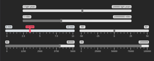
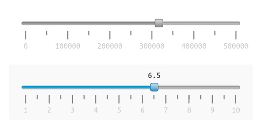
This is a technique I’ve used for styling the output of native range sliders such as the one below.

Styled range input indicating time (live demo)

Time isn’t the only thing we can use this for. Counter values have to be integer values, which means the modulo trick also comes in handy for displaying decimals, as in the second slider seen below.

Styled range inputs, one of which has a decimal output (live demo)

A couple more such examples:

Styled range inputs, one of which has a decimal output (live demo)

Styled range inputs, one of which has a decimal output (live demo)

Even more use cases

Let’s say we have a volume slider with an icon at each end. Depending on the direction we move the slider’s thumb in, one of the two icons gets highlighted. This is possible by getting the absolute value, --abs, of the difference between each icon’s sign, --sgn-ico (-1 for the one before the slider, and 1 for the one after the slider), and the sign of the difference, --sgn-dir, between the slider’s current value, --val, and its previous value, --prv. If this is 0, then we’re moving in the direction of the current icon so we set its opacity to 1. Otherwise, we’re moving away from the current icon, so we keep its opacity at .15.

This means that, whenever the range input’s value changes, not only do we need to update its current value, --val, on its parent, but we need to update its previous value, which is another custom property, --prv, on the same parent wrapper:

addEventListener('input', e => { let _t = e.target, _p = _t.parentNode; _p.style.setProperty('--prv', +_p.style.getPropertyValue('--val')) _p.style.setProperty('--val', +_t.value) })

The sign of their difference is the sign of the direction, --sgn-dir, we’re going in and the current icon is highlighted if its sign, --sgn-ico, and the sign of the direction we’re going in, --sgn-dir, coincide. That is, if the absolute value, --abs, of their difference is 0 and, at the same time, the parent wrapper is selected (it’s either being hovered or the range input in it has focus).

[role='group'] { --dir: calc(var(--val) - var(--prv)); --sgn-dir: clamp(-1, var(--dir), 1); --sel: 0; /* is the slider focused or hovered? Yes 1/ No 0 */ &:hover, &:focus-within { --sel: 1; } } .ico { --abs: max(var(--sgn-dir) - var(--sgn-ico), var(--sgn-ico) - var(--sgn-dir)); --hlg: calc(var(--sel)*(1 - min(1, var(--abs)))); /* highlight current icon? Yes 1/ No 0 */ opacity: calc(1 - .85*(1 - var(--hlg))); }

CodePen Embed Fallback

Another use case is making property values of items on a grid depend on the parity of the sum of horizontal --abs-i and vertical --abs-j distances from the middle, --m. For example, let’s say we do this for the background-color:

@property --floor { syntax: '<integer>'; initial-value: 0; inherits: false; } .cell { --m: calc(.5*(var(--n) - 1)); --abs-i: max(var(--m) - var(--i), var(--i) - var(--m)); --abs-j: max(var(--m) - var(--j), var(--j) - var(--m)); --sum: calc(var(--abs-i) + var(--abs-j)); --floor: max(0, var(--sum)/2 - .5); --mod: calc(var(--sum) - var(--floor)*2); background: hsl(calc(90 + var(--mod)*180), 50%, 65%); }

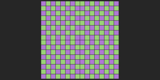
Background depending on parity of sum of horizontal and vertical distances to the middle (live demo)

We can spice things up by using the modulo 2 of the floor of the sum divided by 2:

@property --floor { syntax: '<integer>'; initial-value: 0; inherits: false; } @property --int { syntax: '<integer>'; initial-value: 0; inherits: false; } .cell { --m: calc(.5*(var(--n) - 1)); --abs-i: max(var(--m) - var(--i), var(--i) - var(--m)); --abs-j: max(var(--m) - var(--j), var(--j) - var(--m)); --sum: calc(var(--abs-i) + var(--abs-j)); --floor: max(0, var(--sum)/2 - .5); --int: max(0, var(--floor)/2 - .5); --mod: calc(var(--floor) - var(--int)*2); background: hsl(calc(90 + var(--mod)*180), 50%, 65%); }

A more interesting variation of the previous demo (live demo)

We could also make both the direction of a rotation and that of a conic-gradient() depend on the same parity of the sum, --sum, of horizontal --abs-i and vertical --abs-j distances from the middle, --m. This is achieved by horizontally flipping the element if the sum, --sum, is even. In the example below, the rotation and size are also animated via Houdini (they both depend on a custom property, --f, which we register and then animate from 0 to 1), and so are the worm hue, --hue, and the conic-gradient() mask, both animations having a delay computed exactly as in previous examples.

@property --floor { syntax: '<integer>'; initial-value: 0; inherits: false; } .🐛 { --m: calc(.5*(var(--n) - 1)); --abs-i: max(var(--m) - var(--i), var(--i) - var(--m)); --abs-j: max(var(--m) - var(--j), var(--j) - var(--m)); --sum: calc(var(--abs-i) + var(--abs-j)); --floor: calc(var(--sum)/2 - .5); --mod: calc(var(--sum) - var(--floor)*2); --sgn: calc(2*var(--mod) - 1); /* -1 if --mod is 0; 1 id --mod is 1 */ transform: scalex(var(--sgn)) scale(var(--f)) rotate(calc(var(--f)*180deg)); --hue: calc(var(--sgn)*var(--f)*360); }

Grid wave: triangular rainbow worms (live demo).

Finally, another big use case for the techniques explained so far is shading not just convex, but also concave animated 3D shapes using absolutely no JavaScript! This is one topic that’s absolutely massive on its own and explaining everything would take an article as long as this one, so I won’t be going into it at all here. But I have made a few videos where I code a couple of such basic pure CSS 3D shapes (including a wooden star and a differently shaped metallic one) from scratch and you can, of course, also check out the CSS for the following example on CodePen.

Musical toy (live demo)

The post Using Absolute Value, Sign, Rounding and Modulo in CSS Today appeared first on CSS-Tricks. You can support CSS-Tricks by being an MVP Supporter.

Using Absolute Value, Sign, Rounding and Modulo in CSS Today published first on https://deskbysnafu.tumblr.com/

[chanakyadefence]

How to prepare for NDA 2021 (2) Mathematics

The Mathematics section of NDA will carry 120 objective type multiple-choice questions. Total marks allotted to this section are 300. Candidates will get two hours 30 minutes to solve the question paper. For the correct answer, candidates will score 2.5 marks while 0.83 marks will be deducted for wrong answers.

Syllabus and important topics for Mathematics

NDA syllabus comprises topics from Algebra, Matrices and Determinants, Trigonometry, Analytical Geometry of two and three dimensions, Differential Calculus, Integral Calculus and Differential Equations, Vector Algebra and Statistics and Probability. The topic-wise distribution of questions in Mathematics are given below:

Subjects

Number of Question

Algebra

30

Trigonometry

20

Determinants  and matrices

10

Analytical  Geometry

20

Vector  Algebra

10

Statistics  and Probability

10

Differential  calculus and Integral calculus

20

Total

120

Follow the tips and tricks below for the Mathematics section:

·         Candidates must have a clear understanding of the NDA syllabus and mark the important topics after analyzing the previous years’ question papers.

·         Start preparing the important topics first, at the same time, delegate time for the difficult topics.

·         Solve mock tests to decide how much time to dedicate to each type of question. Also, candidates must solve previous year question papers to get an idea about the type of questions asked in the exam.

·         Candidates must learn tips, tricks and shortcuts for efficient time management.

·         Memorise simple calculations such as squares and cubes.

·         Make notes of shortcuts and formula to refer to during last-minute revision.

·         As there is negative marking in the exam, they should mark the answer only if they are sure about it. Do not guess the answers during the exam.

·         Candidates must refer to good Mathematics books and Coaching classes for NDA preprations.

·         During the final phase of preparation, devote at least three hours for going through the formula.

·         Do not get confused while converting the numbers from decimal to a binary system.

·         Trigonometry can be tricky. So be clear with the concepts such as Properties of Triangles and Inverse Trigonometric functions. Hence, solve such questions at the end.

·         Vector Algebra is the most important unit in the syllabus. Practice questions from Vector Product or Cross Product of two vectors.

·         The statistics part can be easy to crack but be careful while taking the figures.

·         In Probability, the Elementary Theorems, Bayes' Theorem and Binomial Distribution are important.

Best books for Mathematics

It is important that candidates must choose a good book for the Mathematics section of NDA.

·         NCERT Class 11 and 12 books

·         Mathematics for NDA and NA: National Defense Academy and Naval Academy by R S Aggarwal

·         Quantitative Aptitude for Competitive exam by RS Aggarwal

·         NDA and NA examination: Previous solved papers by R Gupta

·         JOIN COACHING CLASSES FOR NDA WRITTEN AND SSB.

·         For better results in NDA written, Join Chanakya Defence Group India’s No.1 Defence coaching institute with renowned faculty from various IIT’s & IIM’s with team of Retd. Defence officers for SSB and Persnality Development sessions. CDG working in the field of NDA, Sainik School, RIMC, RMS, CDS, AFCAT, AIRFORCE & NAVY since 2006 with best results in India. Till now more than 3700+ candidates crack the various defence exam with the help of Chanakya Defence Group.

·         For more Information Kindly contact us at

·         78887-14322 | 85569-70887

·         Website:- www.chanakyadefencegroup.com

·         CLICK:  NDA COACHING IN PATHANKOT

·         Email:- chanakyadefencegroup@gmail.com

[soapybitch]

Dave’s Short Trig Course

Angle in unit circle showing trig functions as lengths of line segments

Table of Contents

Who should take this course?

Trigonometry for you

Your background

How to learn trigonometry

Applications of trigonometry

Astronomy and geography

Engineering and physics

Mathematics and its applications

What is trigonometry?

Trigonometry as computational geometry

Angle measurement and tables

angle theta in a circle of radius r

Background on geometry

The Pythagorean theorem

An explanation of the Pythagorean theorem

Similar triangles

Angle measurement

The concept of angle

Radians and arc length

Exercises, hints, and answers

About digits of accuracy

Chords

What is a chord?

Trigonometry began with chords

sin is opp over hyp

Sines

The relation between sines and chords

The word “sine”

Sines and right triangles

The standard notation for a right triangle

Exercises, hints, and answers

cos is adj over hyp

Cosines

Definition of cosine

Right triangles and cosines

The Pythagorean identity for sines and cosines

Sines and cosines for special common angles

Exercises, hints, and answers

tan is opp over adj

Tangents and slope

The definition of the tangent

Tangent in terms of sine and cosine

Tangents and right triangles

Slopes of lines

Angles of elevation and depression

Common angles again

Exercises, hints, and answers

The trigonometry of right triangles

Solving right triangles

Inverse trig functions: arcsine, arccosine, and arctangent

The other three trigonometric functions: cotangent, secant, and cosecant

Exercises, hints, and answers

Pythagorean triples

graph of sin x

The trigonometric functions and their inverses

Arbitrary angles and the unit circle

Sines and cosines of arbitrary angles

Properties of sines and cosines that follow from the definition

Graphs of sine and cosine functions

Graphs of tangent and cotangent functions

Graphs of secant and cosecant functions

Computing trigonometric functions

Before computers: tables

After computers: power series

law of cosines

The trigonometry of oblique triangles

Solving oblique triangles

The law of cosines

The law of sines

Exercises, hints, and answers

law of sines

Demonstrations of the laws of sines and cosines

For the law of sines

For the law of cosines

Area of a triangle

Area in terms of two sides and the included angle

ptolemy's theorem

Ptolemy’s sum and difference formulas

Ptolemy’s theorem

The sum formula for sines

The other sum and difference formulas

Summary of trigonometric formulas

Formulas for arcs and sectors of circles

Formulas for right triangles

Formulas for oblique triangles

Formulas for areas of triangles

Summary of trigonometric identities

More important identities

Less important identities

Truly obscure identities

About the Java applet.

Images in Dave’s Short Trig Course are illustrated with a Java applet. If your browser is Java-enabled, you can drag the points around in the diagrams and the diagram will adjust itself. The applet also allows you to lift a diagram off the web page into its own floating window. For details, see About the applet.

Note that some web browsers do not allow printers to print images created by Java applets. You may still be able to print the images if turn off Java in your browser, and the plain images should appear that can be printed.

Select topic

Dave’s Short Trig Course is located

at http://www.clarku.edu/~djoyce/trig