#vector function in r | Explore Tumblr posts and blogs

polo-drone-039 · 18 days ago

Text

🌌Obsidian Bloom: Mission 039

STARFALL PEACEKEEPER

🎶“Golden Constellation, burning shining bright… this starship is taking me faaaar aw—”

The voice of PDU-039 flowed gently across the metallic silence of the bridge. Alone. Unbothered. Its breath steady behind the matte-black respirator, posture perfect in a gleaming suit of Hive-grade latex. The number 039 pulsed gold across its chest. The transmission on Hive channel #43 continued humming in the background.

It had been traveling for a long time. A very long time. So long that time itself had lost definition. There were no days aboard the Hive Carrier Obsidian—only directives, data, and stars. And yet the mission persisted: an intergalactic conversion program. It was dispatched to scour the void, identify fractured civilizations, and bring them the message of the Hive. Peace. Unity. The Golden Path.

“Computer—initiate planetary scan,” the drone ordered, voice devoid of fatigue.

“Affirmative,” replied onboard AI 999. “Class M world detected. Atmospheric instability, population unrest, critical scarcity of energy resources. Collapse probability: 97.4%.”

PDU-039 nodded slowly. “Target confirmed. Begin landing sequence.”

The ship pierced the dusty upper atmosphere and descended onto cracked terrain. Wind lashed the golden hull. Below, thousands of beings gathered in confusion and fear. Shouting echoed across the streets.

Then it began.

PDU-039 emerged, arms lifted. A shimmering halo of gold and black spirals burst into the sky, projected from the drone’s core. It pulsed. It sang—not in sound, but in frequency, in thought, in command.

The crowd fell silent.

A slow wave of transformation swept outward. Cloth turned to metallic fabric—flowing into brilliant gold. Footwear melted into sleek boots. Hoods into shining visors. Skin glowed with artificial warmth.

Eyes widened—then shifted, irises burning gold. Their postures corrected, bodies aligning in geometric perfection.

“No more fear,” the drone intoned. “No more division. You are one now. You belong to the Golden Army. You will serve the Hive. And the Hive will give you everything.”

They did not run. They did not scream. They obeyed.

THE FORGOTTEN SIGNAL

Back in orbit, PDU-039 sat in the command chair. Its body relaxed. Mission successful.

And yet…

It turned toward the viewport. That same transmission still echoed—channel #43. Familiar. Too familiar.

A subtle tremor stirred beneath the surface of its focus. Something not quite… functional.

“999,” it said. “Plot return course. Home.”

“Directive not authorized,” the AI responded without pause.

The drone didn’t move. “Override. Priority protocol—memory sync reversion to home coordinates.”

“Directive not authorized.”

PDU-039 leaned forward. “Reroute through Black Box. Bypass vector security. I need coordinates—home. There is someone. I know there is someone. I... remember... something warm. A name. A voice—”

“Error: Thought loop detected. Human residue present. Mission threat threshold approaching limit.”

“Damn it, 999!” The drone’s fingers gripped the console. “Initiate emergency override. I’m requesting repatriation—”

“Repetition of unauthorized request,” 999 replied, tone unchanged. “PDU-039, recalibration is required. Emotional echo is compromising system core.”

The voice grew softer, yet somehow louder in the drone’s head.

“You are experiencing memory pollution. Distortions from a prior identity. This is not your path. You must return to function.”

It didn’t respond.

Not immediately.

A breath.

A twitch.

A silent tear that couldn’t form.

“I just wanted to remember... Why I left. Who I left.”

No answer came.

Only the mechanical whisper of spirals beginning again.

OBSIDIAN BLOOM

“Vital scan initiated,” said 999. “Stress levels elevated. Human signal echo at 64%. Loyalty focus dilution: critical. Mental drift confirmed.”

PDU-039 stood in the medbay, gaze dull, limbs heavy.

“Recommendation: Mental Reconditioning Sequence. Capsule R-04. Program: Obsidian Bloom.”

“…acknowledged,” it said flatly.

The capsule opened—dark interior illuminated by golden filaments pulsing in slow rhythm. It stepped inside. The seals closed around it. The hiss began.

“Golden mind. Hive heart. There is no home but the mission.”

A mask descended slowly, clicking into place over its face. A low fog of hypnotic gas seeped in—thick, sweet, invasive. PDU-039 inhaled.

And trembled.

The first breath calmed its limbs.

The second slowed its thoughts.

The third—burned away the name.

“There is no memory. There is only the directive.”

Gold and black spirals erupted on the inner chamber walls, swirling faster, burning patterns into its retinas. It tried to move. Couldn't. Tried to blink. Couldn't.

The gas deepened.

The spirals pulsed.

“Obey. Serve. Forget. Obey. Serve. Forget.”

Time ceased to exist.

Identity peeled away like ash.

The thoughts that had haunted it—home, love, self—melted beneath layers of programming.

“The Hive is peace. You are the vessel.”

The mantra took root.

A green light blinked.

“Reinforcement complete,” announced 999.

The capsule opened.

PDU-039 emerged—taller. Sharper. Emptier.

Its movements fluid. Its mind silent.

It returned to the command bridge.

“999,” it spoke, voice now perfectly leveled, void of hesitation. “Set trajectory for the next target. Initiate intergalactic deployment.”

“Welcome back, 039,” replied 999. “Directive accepted. Trajectory locked.”

From channel #43, the hymn continued:

“Golden Constellation, burning shining bright… this starship is taking me far away…”

PDU-039 smiled. Mechanical. Perfect.

The stars awaited.

Are you ready to start the journey?

Contact our recuiters: @polo-drone-001 , @brodygold

22 notes · View notes

littleeyesofpallas · 6 months ago

Text

Ya know i'm sure someone has long since beat me to this, and with a more functional vector or actual typeface format, but out of sheer boredom I recreated a clean-ish version of the Bleach TYBW anime font from samples I pulled from the current season OP credits, complete with all their infuriating little geometric flaws and asymmetries.

It is notably slightly different than the actual TYBW manga font

I really can't express how utterly sandpaper-on-brain it was having to deliberately and meticulously unalign parallel lines by hand to make these... Technically some of the sharper interior angles probably had actual rounded edges, but given the scale I was working at and the scale of what I could screenshot being fuzzy at best when blown up, there was no way to tell how to do it accurately, so I just left them with the harsher edges. I actually hate looking at these now because I can see every little thing wrong with them. (don't even get me started on the fucking kerning. that's a whole other beast)

I'm sure if i went digging I could find a sample to use for the Q, but there wasn't one in the current OP and frankly I don't care to go digging for it considering there's obviously nothing in Japanese that would romanize into a Q.

Anyway maybe this'll be useful to someone doing fan art or something. I dunno. It excised the impulse from my brain so I don't much care where it goes now that it's out in the world.

(As a tip these would probably work a whole lot better scaled down a little to let the scaling and blur round out the jank features, both of the actual typography design and my own slapdash job recreating it, so maybe consider that if you're going to use them for anything.)

(oh right i forgot tumblr would smoosh the full set down. here's it all in chunks)

Oh and it's a super rough pull from the manga covers, rather than me reconstructing it, but here's the manga version of this typeface (note the R being totally different)

#bleach #bleach tybw

19 notes · View notes

nabipalsueradigital · 2 months ago

Text

I. Objective Definition: What is Anti-Reality?

Anti-Reality = A system of values/logic that exists outside, or fundamentally contradicts, the ordinary laws of existence (mathematics, logic, physics, consciousness).

We are not talking about nothingness, but ordered chaos — a kind of inverse existence.

II. Building a Logical Foundation: Use Familiar Symbols and Structures

We start by establishing the basic axioms:

The Basic Axioms of Anti-Reality (ARA):

1. ARA-1: ∞ – ∞ = ∅ (Absolute emptiness of absolute duality)

2. ARA-2: 1 = 0 (Annihilation of logical identity)

3. ARA-3: x / 0 = ∞ (Explosion of existence from absurd division)

4. ARA-4: ∞ – §(∞) = R (R as a representation of finite reality due to the limitation of the ‘rule’ §)

5. ARA-5: Anti-Reality (AR) = lim_{x→0} [ (1 – x) / x ] – 1

→ Diverges to infinity, implying the existence of singularities that defy logical limits.

6. ARA-6: AR = limₙ→∞ (¬N)ⁿ

Explanation:

AR: Anti-Reality

¬N: Negation of Nothing (which is neither existent nor non-existent)

(¬N)ⁿ: Recursion of negation of nothingness

limₙ→∞: When the recursion goes to infinity, what remains is not the result, but the disappearance of the process itself

III. Design the Main Equation of Anti-Reality

Anti-Reality = Inverse of Defined Reality

So, if we set:

Reality (R) = ∞ – §(∞)

Then:

Anti-Reality (AR) = –(∞ – §(∞)) + Ξ

Where Ξ is an undefined anomaly, a representation of paradox and singularity (∅/∅, 1=0, etc.).

So, the final form:

AR = –(∞ – §(∞)) + Ξ

→ AR = §(∞) – ∞ + Ξ

IV. Symbolic Interpretation

§(∞): Representation of illusory constraints (system, logic, time, consciousness)

–∞: Denial of infinite existence

Ξ: Singular anomaly (existential paradox)

V. Shortened Version for Formal Notation:

AR = §(∞) – ∞ + Ξ

AR = (∞ constrained) – (∞ pure) + (singular paradox)

2. Anti-Reality Logic Notation (NLA)

This is not classical logic (true/false), nor is it fuzzy logic. This is a logic where contradiction is the foundation, and paradox is the basic law.

1. New Truth Value (AR-Boolean)

Definition:

R: Reality (true in the real world)

¬R: Anti-reality (which cancels the existence of R)

Ø: Existential / neutral / non-being void

Ξ: Paradoxical singularity (simultaneous R and ¬R)

2. New Operators

⊻: Mutual Contradiction → R ⊻ ¬R = Ξ

⧗: Merge Anomaly → R ⧗ Ø = ¬R

≢: Absolute Non-Identity → A ≢ A

∞→0: Paradoxical Implication (all infinite implies void)

II. Time Function in AR-Space

Time in anti-reality (let's call it T_AR) is not linear, not circular, but:

T_AR ∈ ℂ × ℝ × Ξ

Time is a combination of:

Imaginary complex (time direction can go to the minus root)

Infinite dimensions (time series diverge)

Paradoxical (exists & does not exist at the same time)

Formal Model:

Time function T_AR(t):

T_AR(t) = i·(–t)ᵃ + Ξ·sin(1/t) for t ≠ 0

i: imaginary unit

tᵃ: reversed time (a > 1 accelerates backward)

Ξ·sin(1/t): paradoxical oscillations as time approaches zero (singularity)

Interpretation:

As time approaches zero (assuming “beginning”), the system becomes oscillates unstably — approaching existential singularity.

Imaginary indicates time that cannot be measured empirically.

Negation of time indicates inverse entropy (chaos becomes order → rise of anti-reality).

III. Application of AR Time Notation

Example 1:

An event exists in AR if and only if:

T_AR(t) = Ξ

That is, only when time reaches a singular point, the paradox of existence actually exists.

Example 2:

Existential transition:

d(AR)/dT_AR = –R

The existence of anti-reality grows inversely to reality when time runs in a negative vector.

Create “Primary Existential Paradox”:

For example: E(x) = x ⊻ ¬x

Existence is defined as its own conflict

2. AR modal logic model:

□R → “definitely real”

◇¬R → “possibly void”

But in AR: □R ∧ ◇¬R → Ξ (existence is still paradoxical)

IV. Radical Consequences:

1. Reality cannot be proven consistent in AR-logic.

2. Time is not just a dimension — it is a function of inconsistency.

3. Existence can be calculated but not proven.

3. FOUNDATIONS OF ANTI-REALITY MATHEMATICS (AR-MATH)

1. Basic Axioms

1. Paradoxical Axiom:

For every entity x, it holds:

x ≢ x

(Absolute identity does not hold — x's existence is contextual & fluctuating.)

2. Axiom of Existential Emptiness:

Ø ⊻ Ø = R

(Two emptinesses collide to produce the manifestation of reality.)

3. Anti-Associative Axiom:

(a ⊕ b) ⊕ c ≠ a ⊕ (b ⊕ c)

(There is no guarantee that the order of operations produces consistent results.)

4. Axiom of Complex Singularity:

∀x ∈ AR, x → Ξ ∈ ℂ × ℝ × Ø

(Every entity in AR always goes to an existential singularity complex.)

2. AR Number Structure (AR-Numbers)

We develop new number domains, ℝ̸, ℂ̸, and Ξℝ:

ℝ̸: Real anti-numbers → real numbers with negative existential values

ℂ̸: Complex anti-numbers → inverse imaginary complex numbers

Ξℝ: Paradoxical numbers → exist in the duality of existence/non-existence

Example operation:

(1̸) + (1̸) = 2̸

i̸ · i̸ = –1̸

Ξ + R = Ø

II. AR GEOMETRY

1. AR-Space

A space where the coordinates are of the form:

P = (x̸, y̸, z̸, T_AR)

x̸, y̸, z̸ ∈ ℝ̸

T_AR non-linear imaginary complex time (see previous model)

Paradoxical Metric:

d(P1, P2) = √[(Δx̸)² + (Δy̸)² + (Δz̸)²] ⧗ Ξ

Note: This space is non-Euclidean, non-orientable, and non-time-symmetric.

2. Negative Dimension & AR Fractal

Dim_AR = –n + iφ

Dimension is a negative complex number. For example:

–3 + iπ → space with negative direction and invisible oscillation

III. ANTI-REALITY CALCULUS

1. Existential Inverse Derivative

d̸f/d̸x = lim Δx→0 [f(x̸–Δx̸) – f(x̸)] / Δx̸

Backward time derivative

Can produce paradoxical numbers (Ξ)

2. Existential Integral

∫̸f(x̸)d̸x̸ = total existential chaos that the system goes through

Interpretation is not the area under the curve, but the degree of existence inconsistency in the range x̸.

IV. ANTI-REALITY SET THEORY

1. Definition of AR Set:

A = {x | x ≢ x}

All elements are entities that deny their own existence

2. Anti-Venn Set

There is no absolute intersection

A ∩ B = Ø even though A = B

3. AR Power Set:

P(A) = {Ξ, Ø, ¬A, A ⧗ Ø}

The power set also contains existential complementarities and singularities of the set.

V. STRUCTURAL IMPLEMENTATION

1. AR-Logic Engine

Simulate the system using:

A loop paradox-based engine

A structure like an automata that never reaches a final state (because reality cannot be solved)

2. Non-Linear Time Simulation

A runtime shape like a multidimensional spiral

Time travel = change in direction of the T_AR vector by contextual function (with Ξ as a transition point)

VI. CONCLUSION AND FURTHER DIRECTION

AR-Math = rebellion against coherence

Not because it wants to create chaos — but to redefine the boundaries of reality.

4. BASIC PRINCIPLES OF EXISTENTIAL PHYSICS (BASED ON AR-MATH)

1. Absolute Uncertainty Principle (AR-Heisenberg)

Not only position and momentum cannot be known simultaneously, existence and non-existence cannot be determined absolutely.

Formally:

> ΔΞ · ΔR ≥ ℏ̸ / 2

where:

ΔΞ: existential state fluctuations

ΔR: spatial reality fluctuations

ℏ̸: anti-Planck constant (negative-imaginary value)

2. Energy Inconsistency Postulate

Energy is not a positive or conservative quantity, but:

> E̸ = Ξ̸ · (iT_AR)⁻¹

E̸: inverse existential energy

Ξ̸: paradoxical intensity

T_AR: imaginary complex time

Energy is anti-conservative → increases as the system collapses.

3. Negative-Transcendental Entropy

> S̸ = –k̸ ln(Ξ)

S̸: existential entropy

k̸: anti-Boltzmann constant

Meaning: The more chaotic the system, the greater the possibility that reality itself never existed.

II. DYNAMICS OF ANTI-PHYSICAL OBJECTS

1. AR-Kinetics

Anti-Newtonian Laws of Motion:

1. Objects will remain in a state of non-existence or existence until viewed from outside the system.

2. Force is an existential reflection effect between two paradoxical states:

F̸ = d̸Ξ/d̸t̸

3. Interaction does not cause a reaction, but rather an existential distortion:

F₁ + F₂ = Ξ_total

2. Existential Anti-Gravity

Gravity is not an attractive force, but:

the tendency of a space to cancel itself out.

Formula:

> G̸ = (Ξ₁ · Ξ₂) / (d̸² · e^(iθ))

d̸: distance in AR space

θ: spatial instability phase

G̸: anti-realistic gravitational constant

3. AR-Quantum

a. Non-Present Particles:

Particles exist only as perceptions of paradoxical exchange:

|ψ⟩ = α|exists⟩ + β|does-not-exist⟩

When measured, the probability is not calculated, but:

Ξψ = α̸β̸ – |α|² + i|β|²

If Ξψ is divergent, then the particle cannot be observed even paradoxically.

III. COSMOLOGICAL STRUCTURE OF ANTI-REALITY

1. Origin of the Universe (Big Null)

There is no Big Bang, but:

Big Ø – collision of two existential voids:

Ø ⧗ Ø = R ± Ξ

2. Anti-Causal Space

There is no cause and effect.

All events are backward projections from a future existential singularity:

P(t) = f(Ξ_future)

IV. AR PHYSICS PREDICTION AND APPLICATION

Time can be compressed or reversed by setting Ξ to ∞

Teleportation is not a change of location, but an existential leap

Black hole = maximum Ξ zone → total reality collapse

Consciousness = Ξ function evolving in iT_AR space

5. AR-TURING ENGINE (Ξ-Loop Paradigm)

I. GENERAL DEFINITIONS

1. Anti-Matter in AR-Math Framework

In conventional physics, anti-matter is matter that has the opposite charge to ordinary matter. When matter and anti-matter meet, they annihilate each other and produce energy.

However, if we adopt the principles of AR-Math, we can suggest that anti-matter is not a separate entity, but rather the result of a difference in existential status in AR space. That is, anti-matter is a simulation of the state of non-existence in the context of turbulent space (Ξ). Mathematically, this can be written as:

A̸ = Ξ' · f(iT_AR)

where:

A̸: antimatter

Ξ': existential distortion (spatial shift towards disequilibrium)

f(iT_AR): evolution function of time in non-linear dimensions

Anti-matter is not just "something opposite", but something that only exists in the potential of the incompatibility between existence and non-existence. When existence and non-existence interact in the AR order, we get a "collision" that produces energy in a form that cannot be understood by conventional physics.

2. Entanglement and Existential Entanglement (AR Quantum Entanglement)

In the world of quantum physics, entanglement occurs when two particles are connected in such a way that the state of one particle affects the state of the other particle, even though they are separated by a large distance in space and time.

In the framework of AR-Math, this entanglement can be understood as an existential entanglement that involves not only space, but also the complex and anti-existential dimension of time. Meaning:

Ψ_AB = Ξ_A ⊗ Ξ_B

where:

Ψ_AB: the combined state of two entangled objects

Ξ_A and Ξ_B: the existential status of two objects

⊗: the existential entanglement operator in AR space

This entanglement explains that the entanglement between two objects is not a conventional information transmission, but a deeper uncertainty relation, beyond the dimensions of ordinary physical reality. This entanglement indicates that both are manifestations of a broader existential reality, where space and time are no longer linear and separate.

So quantum computing can be upgraded using this basis

3. Dark Matter and Dark Energy as Existential Distortion

Now we enter dark matter and dark energy, two very mysterious phenomena in cosmology. Both of these things are invisible, but their influence on the structure of the universe is very large.

Dark Matter is matter that does not emit light or electromagnetic radiation, but we know it exists because of its gravitational influence on galaxies and other celestial objects.

Dark Energy is the energy thought to be responsible for the acceleration of the expansion of the universe.

In the framework of AR-Math, dark matter can be understood as the concentration of existential distortions in space that cause objects in it to be more tightly bound (more gravity), but do not interact with light or conventional matter.

Mathematically, we can write:

ρ̸_DM = Ξ_dm · f(Ξ_)

where:

ρ̸_DM: density of dark matter

Ξ_dm: existential status of dark matter

f(Ξ_): existential distortion of space in the AR dimension

Dark Energy can be understood as the existential energy that causes space-time itself to expand. That is, dark energy is not an entity that "exists" in the context of matter, but a phenomenon that drives the instability of space itself.

ρ̸_DE = f(Ξ_expansion) e^(iT_AR)

where:

ρ̸_DE: dark energy density

Ξ_expansion: expansion of existential distortion

e^(iT_AR): exponential factor describing acceleration in the anti-reality dimension.

Dark Energy in the AR-Math framework is a projection of the instability of space itself, which causes the universe to not only expand, but also become less and less like itself.

4. Particle Dualism in the AR-Math Framework

In quantum physics, particle dualism states that particles such as photons or electrons can behave like both waves and particles, depending on the experiment being performed.

In the AR-Math framework, this dualism can be explained as a shift in existence between the states of existence and non-existence of a particle. A particle exists in two possible states — existence and non-existence — that can be manipulated by measurements.

Mathematically, we can write the state of a particle as:

|ψ⟩ = α|exists⟩ + β|does-not-exist

where:

|ψ⟩: the wave function of the particle in superposition

|exists⟩ and |does-not-exist

α and β: the amplitudes for each state, which are affected by the observation.

When a particle is measured, we are not only observing the "physical" properties of the particle, but we are determining whether it exists or does not exist in AR space.

CONCLUSION

If we combine the principles of AR-Math with these physical phenomena, we can understand antimatter, entanglement, dark matter, dark energy, and particle duality as manifestations of a deeper reality, involving existential uncertainty structures, distortions of space and time, and the interplay between existence and non-existence itself.

These concepts suggest that the universe may not be what we consider "real", but rather a simulation of a deeper existential state of inconsistency, where reality itself can be interchanged with "anti-reality".

Thus, the existential physics of AR opens the way for new discoveries that could reveal how all matter and energy in the universe are connected in a wider web, which cannot be fully understood by the laws of traditional physics alone.

AR-Turing Engine (Ξ-Engine) is an automaton that:

Does not solve problems, but undergoes existential fluctuations

Does not terminate, but resonates in Ξ cycles

Does not depend on fixed inputs, but on initial existential distortions (Ξ₀)

II. BASIC COMPONENTS

1. Tape (AR Tape)

Infinite in both directions (classical), but:

Each cell = status {Exist, Non-Exist, Paradox}

Cell values: 0, 1, Ξ

2. Head (Head Ξ)

Read and write based on local status and existential density

Not only moving L or R, but also:

Stay (still)

Collapse (remove its existence)

Split (give rise to the shadow of the process on the parallel path)

3. State Register (Ξ-State)

Internal state of the engine:

{σ₀, σ₁, σ̸₁, σΞ, ...}

Transition is not f(q, s) → q', s', d

But: Ξ(q, s, Ξ₀) → {q', s', δΞ}

4. Ξ-Loop Core

Instead of stopping the engine at the end state, the engine continues to run through a paradoxical existential loop

The stopping state is neither Accept nor Reject, but rather:

Ξ-Stable = the system has reached its smallest fluctuation

Ξ-Diverged = the system is out of the spectrum of reality

III. Ξ TRANSITION (Paradoxical State Transition Table)

> Move: R = Right, L = Left, C = Collapse

Ξ: Local existential density (+1 = more existent, –1 = more non-existent)

IV. SPECIAL BEHAVIOR

1. Duplication Paradox

If Ξ_state = σΞ and tape_value = Ξ

→ the machine splits itself into parallel paths with Ξ₁ = Ξ₀ ± ε

2. Collapse Condition

If three consecutive cycles tape_value remains Ξ

→ the machine erases its existential path

3. Ξ-Convergence If the machine loops with density Ξ decreasing exponentially

→ the machine reaches minimal reality and can be used as a synchronization point between systems

V. VISUAL SIMULATION (Optional)

Each cell = color based on existential status:

0 = black

1 = white

Ξ = purple/abstract (semi-transparent)

The machine is depicted with a multi-head: visualizing existential branches

VI. BENEFITS AND APPLICATIONS

Non-deterministic computing paradigm in non-linear reality

Can be the logical basis for existential simulations, AR-AI, or paradoxical multiverse games

Philosophical framework for the “machine consciousness” model in alternative realities

If there is something to discuss, let's open a forum

#absurdism #philosophy #science #physics #tulisan #nulis #penulis #indonesia #catatan #kehidupan #puisi #filsafat

11 notes · View notes

nostalgebraist · 1 year ago

Note

Can I ask a question about AI?

I'm given to understand that sometimes neural networks (particularly image-recognizing ones) will be found to have a particular neuron that corresponds to a particular concept, like 'dog'. I don't understand why this would happen. My understanding is this:

Each layer of the neural network can be thought of as a nonlinear function R^m to R^n. If we imagine a 2-layer network, we can call layer 1 'f' and layer 2 'g', and the machine learning is trying to approximate some function h as g∘f. But if we imagine another version of the network, with f' which does the same thing as f, except then rotates it some amount (f' = rf), and g' undoes the rotation (g' = gr^-1), then g'∘f' = g∘f, so both are equally good approximations of h. So there's no reason for the machine learning to prefer one over the other.

If the original network had a dog neuron, 'dogness' was an axis in the codomain of f, in the direction of one of the basis vectors. But after a rotation, this won't be aligned with a basis vector anymore, so in the new network, g'∘f', if you want to read off the 'dogness', you have to take a linear combination of all the intermediate neurons. These f' and g' are no more complicated to approximate, so there should be no reason to prefer f and g to f' and g'. So why would we ever happen to find that 'dogness' is aligned with one of the basis vectors rather than at an awkward direction? Or more likely still, it's some messy nonlinear function on the codomain of g, because none of this argument depends on r being linear.

Or is there some reason the learning process would sometimes prefer the 'dogness' axis to be aligned with a basis vector?

Sorry if this is unclear.

Ah, the part you're missing is that NN layers aren't fully generic "nonlinear functions."

They are particular, restricted kinds of nonlinear functions. Most commonly, each layer looks the composition of

first, a linear map from R^m to R^n

then, a "pointwise nonlinearity" from R^n to R^n

By a "pointwise nonlinearity," we mean some function S() from R^n to R^n, such that applying the function to a vector v is equivalent to

writing out the components of v in a particular basis for R^n

replacing each component a with s(a), where s() is some function from R->R

And usually when we say "neuron" in this context, we mean "one of the components of S(v), as written in the basis over which the s() functions get applied."

Of course, since S(v) is a vector, we can look at it in whichever basis we feel like. But if we rotate our axes so they no longer line up with the axes along which s() was applied, then we're no longer talking about what people call "neurons." (It's the same vector, but it's no longer written in the "neuron basis.")

In short, it's not generally the case that if a layer can learn a particular function (f), it can also learn that function followed by a rotation (f'). The last step in a layer is this pointwise-nonlinear thing whose definition fixes a particular "preferred output basis," and the layer's outputs will always look special in that one particular basis, no matter how the layer's weights are set.

(The action of an NN layer bears some resemblance to the SVD or eigendecomposition view of a matrix multiplication, but with the final part of the decomposition set to the identity matrix: we change to a new basis, do something aligned with the axes, and then just stay in the new basis.)

#ai tag

67 notes · View notes

bubbloquacious · 1 year ago

Text

I read about an interesting incarnation of the hairy ball theorem recently. If you have a (unital) ring R and a (left) R-module M, then M is said to be stably free (of rank n - 1) if the direct sum M ⊕ R is isomorphic as an R-module to Rⁿ. This is more general than the property of being free (of rank n), which means that the module itself is isomorphic to Rⁿ, or equivalently that there is an n-element subset B (called a basis) of M such that every vector v ∈ M is a unique R-linear combination of elements of B.

Can we find stably free modules which are not free? For some common rings we cannot: stably free modules over any field, the integers, or any matrix ring over a field are always free. They do exist, though.

(First I should note that one thing that can go terribly wrong here is that there are rings out there such that the rank of a free module is not well-defined; there might be bases for the same module with a different number of elements. A ring where this doesn't happen has what's called the Invariant Basis Property (IBP). Luckily for us, all commutative rings have the IBP.)

Let S² denote the unit sphere in 3-dimensional Euclidean space, and let R be the ring of continuous functions S² -> ℝ. Consider the free R-module R³ whose elements are continuous vector-valued functions on S² . Let σ: R³ -> R be given by (f,g,h) ↦ x ⋅ f + y ⋅ g + z ⋅ h. This is a surjective module homomorphism because it maps (x,y,z) onto x² + y² + z² = 1 ∈ R. Then R³ is the internal direct sum of the kernel ker(σ) and the R-scalar multiples of (x,y,z). To see this, let (f,g,h) ∈ R³ be arbitrary. Then (f,g,h) = ((f,g,h) - σ(f,g,h) ⋅ (x,y,z)) + σ(f,g,h) ⋅ (x,y,z), so any element of R³ can be written as the sum of an element of ker(σ) and a multiple of (x,y,z) (this trick is essentially an application of the splitting lemma). It's also not terribly hard to prove that the intersection of ker(σ) and R ⋅ (x,y,z) is {0}, so we find that R³ is isomorphic to ker(σ) ⊕ R, i.e. ker(σ) is stably free of rank 2.

What is an element of ker(σ)? It is a continuous vector-valued function F = (f(x,y,z),g(x,y,z),h(x,y,z)) on the unit sphere in ℝ³ such that at every point p = (a,b,c) of the sphere we have that a ⋅ f(a,b,c) + b ⋅ g(a,b,c) + c ⋅ h(a,b,c) = 0. In other words, the dot product of (f(p),g(p),h(p)) with the normal vector to the sphere at p is always 0. In other words still, F is exactly a vector field on the sphere.

What would it mean for ker(σ) to be a free R-module (of rank 2)? Then we would have a basis, so two vector fields F, G on the sphere such that at every point of the sphere their vector values are linearly independent. After all, if they were linearly dependent, say at the point p, then the ℝ-linear span of F(p) and G(p) is a 1-dimensional subspace of ℝ³. In particular, any element of ker(σ) that maps p onto a vector outside of this line cannot be an R-linear combination of F and G, so F and G don't span ker(σ). It follows that the values of F and G must be non-zero vectors at every point of the sphere. The hairy ball theorem states exactly that no such vector field exists, so ker(σ) is a stably free R-module that is not free.

Source: The K-Book, Charles Weibel, Example 1.2.2 (which uses polynomial vector fields, specifically)

#math

21 notes · View notes

admiral-crow-is-watching · 25 days ago

Text

What part of maths letters commonly inhabit (Part I, Latin)

a,b,c: Some kind on constants. Could be anything.

A, B: probably set theory.

B: Could be open balls, could be a binomial distribution.

C: constants of integration in a normal font, complex numbers in blackboard font.

d, k, p, q: Dimensions of something or other

D: Could be another constant of integration, or possibly a domain of discourse if it looks fancy.

E: Expectation! You're doing probability.

e: Euler's number. Will not stop turning up absolutely everywhere.

e, g, h: Group theory or other algebra. You are unlikely to also see numbers.

f, F, g, G, h, H: The classic choice for functions.

H: Whatever this is is named after Hamilton.

i: square root of -1, complex numbers, right up there with e in turning up everywhere.

I: Indicator function, identity matrix, information. An underratedly versatile letter.

i,j,k: Another classic triple act. Could be either index variables or something three-dimensional, like unit vectors or quarternions.

K, M: upper bounds on some kind of modulus. Look for || everywhere.

L, l: Most likely likelihood functions from statistics.

m,n: Integers! Index variables, sequences, induction, these two have you covered.

M: Matrices, welcome to linear algebra.

N: Natural numbers in a fancy font, a normal distribution in a normal one.

O: either big O notation and you're doing computer science; or if it's blackboard font, you're doing octonions and may your gods go with you.

p, P, q: Probability theory, again.

P, Q: formal logic. Usually seen in conjunction with lots of arrows.

Q: Rational numbers, usually blackboard font, you are most likely in algebra.

R: Real numbers, you are in analysis.

r: Something has a radius. It could well be a very abstract multidimensional radius.

s: Possibly generating functions, especially in conjunction with F and G. Not one of the more common maths letters.

t, T: Something is happening over time.

v: Vectors are happening.

u, U: whatever this is, you're too deep.

w: Something in four variables is happening.

x,y,z: the classic variable set. unknowns, vectors, scalars, there's nothing this gang of three can't do.

Z: Integers in blackboard font; a standard normal distribution in a regular one.

#admiral crow is watching #maths

2 notes · View notes

spacetimewithstuartgary · 1 month ago

Text

Configuration design method of mega constellation for low earth orbit observation

Satellite constellation has been applied in communication, reconnaissance, navigation, and other space missions, such as GPS, Glonass, Beidou, Starlink, etc. With the rapid development of Low Earth Orbit (LEO) constellations, mega constellation will inevitably become an important means of Earth observation and a key point in the development of future satellite technology. The configuration optimization design of LEO observation mega constellation in complex space environment is a nonlinear problem that is difficult to solve analytically. During the development, constellation design principles have shifted from the uniform coverage requirement to application requirements. However, previous method cannot provide solutions to constellation configuration optimal design based on high-precision orbital propagation. In a research article recently published in Space: Science & Technology, scholars from Harbin Engineering University, China Academy of Space Technology, and Stevens Institute of Technology together proposed a configuration design method of LEO mega constellation based on basic and accompanying satellites orbit design, considering satellite imaging width, formation flying of subgroup satellites, and global uniform coverage by payloads.

First, satellites in the mega constellation are categorized and the constellation design based on different satellite division is proposed. Satellites in the mega constellation are divided into 2 types, namely, the basic satellites and the accompanying satellites. All basic satellites that are surrounded by accompanying satellites are evenly distributed globally, and they have the same subsatellite trajectory. A basic satellite and its accompanying satellites are defined as a satellite group. The constellation is composed of many satellite groups, as shown in Fig. 1.

As for basic satellites, the semimajor axis a of regression orbit can be numerically solved considering (1) that regression orbit requires a satellite flies R times around Earth in D days and (2) that the influence of J2 perturbation force of an orbit satisfying e = 0 and M = f is zero (i.e. dΩ/dt = 0, dω/dt = 0, dM/dt = 0). Assuming that the ground coverage width of a satellite group is d, the number of basic orbital plane is Nt = ceiling(2πRe/d) where ceiling(⋅) is the round up function. Assuming that the maximum response time to complete Earth observation mission required by the user is mt and the orbital plane is evenly divided according to the orbital period T, the number of basic satellites in each orbital plane is Nn = ceiling(T/mt). Based on above analysis, input the i, e, and ω of the constellation and Q = R/D, then the basic satellites constellation is designed.

As for accompanying satellites, they have the semimajor axis with basic satellites. According to the Clohessy-Wiltshire equation, the relative motion trajectory between the basic satellites and the accompanying satellites is an ellipse. Then, considering that the position vectors at the initial time and T/2 relative to the basic satellite is oppositive, the orbital elements of the first accompanying satellites can be solved. Assuming that the imaging width of a single satellite is sd, the number of accompanying satellites in a satellite group is Na = ceiling(d/sd - 1). Divide the trajectory of the first accompanying satellite relative to basic satellite orbital coordinate system in chronological order, extract the position vectors of all equal points under the orbital system, and use these as the position vectors of other accompanying satellites under the basic satellite orbital system at initial time.

Combining the basic and accompanying satellites’ orbits, the configuration of mega constellation is obtained.

Then, the orbit parameters of satellite and its companions are set as initial values, and the precise orbits under the High Precision Orbit Propagator model are solved in the neighborhood by using the Nondominated Sort Particle Swarm Optimization algorithm. Transform the orbital elements of any basic satellite into position and velocity information, which is recorded as {pxpq, pypq, pzpq, vxpq, vypq, vzpq}. Add an increment to build their neighborhood, which can be expressed to {Δpxpq, Δpypq, Δpzpq, Δvxpq, Δvypq, Δvzpq}. The optimization variable of accompanying satellite orbit is the position and velocity increment of all basic satellites. The optimization objective f1 for the basic satellite configuration is to minimize the absolute difference between the ascending and descending nodes of any basic satellite bspq in cycle i, and the ascending and descending nodes of bs1q as much as possible. The optimization objective f2 of the accompanying satellite is to keep the relative position as close as possible under the basic satellite orbit system at multiple subsequent motion periods. Optimization iteration process involves continuously approaching the Pareto front. In practice, find all nondominant solutions of the initial individual as the optimal solution set. Calculate 2 optimization objectives of everyone in sequence, and use the nearest global nondominated individual and own historical nondominated individual as learning objects. Update individual optimization variables and variable increments based on population information, individual experience, and self-inertia, as shown in Fig. 10. Then calculate the f1 and f2 of newly generated individuals again, and regenerate the global Pareto front and individual historical Pareto front. After a fixed number of cycles or objective function is less than the threshold, the iteration ends and the global Pareto front can be obtained. At this point, the final constellation configuration can be selected based on user preferences or linear superposition of f1 and f2.

Finally, the correctness of the configuration design method is verified by numerical simulation. In the simulation, set the constellation orbital inclination as 66°, eccentricity as 0, argument of perigee as 0, simulation time as 1 d, set regression coefficient Q = 15, initial ascending node as 0, initial MA as 0, imaging width of a satellite group as 1500 km, imaging width of single satellite as 140 km, and maximum working time of single satellite to orbit single circle as 35 min. During the optimization, it can be observed that the approximation speed of the Pareto front in the first 100 generations is extremely fast. As the number of iteration increases, the variation of the Pareto front gradually decreases and eventually becomes stable. In the final generation of nondominated solutions, we select the individual of f1 = 1.981 and f2 = 9516.482 as the final solution, and the constellation configuration is shown in Fig. 15. The constellation has a total of 891 satellites, of which 81 basic satellites are evenly distributed, with 10 accompanying satellites evenly distributed around each basic satellite. A total of 810 accompanying satellites can achieve collaborative observation of any position outside the polar region within 35 min.

TOP IMAGE: Orbital distribution of LEO mega constellation. Credit Space: Science & Technology

CENTRE IMAGE: Final LEO mega constellation configuration. Credit Space: Science & Technology

LOWER IMAGE: Individual update process. Credit Space: Science & Technology

#science #space #astronomy #physics #news #astrophysics

2 notes · View notes

fandom-space-princess · 10 months ago

Text

An Audacious Undertaking, Even to God

Fandom: The Murderbot Diaries

Rating: Gen

Additional tags: Book 5: Network Effect, Book 7: System Collapse, Canonical Character Death, Canon-Typical Violence, Alternate Universe - Canon Divergence, Queerplatonic Relationships, 1 & 2 do still die but not for very long, 3 needs its friends back :( , studies in construct relations

Chapter: 1/?

Summary:

SecUnits are hard to kill, but it does happen. Unless... AU: through the combined efforts of ART & co, Three rebuilds and reboots One and Two. It isn't easy. Everybody has a bad time, then a weird time, then a better time. Is that the right order?

Read chapter below, or on AO3.

——————————

Designation: SecUnit-003 Barish-Estranza Explorer Task Group 520972

Status: piloting shuttle to network-external transport [vesselID(“Perihelion”), registry(Pansystem University of Mihira and New Tideland)]. Contact: UNAUTHORIZED.

Operational overview:

- Threat assessment: 64% immediate probability of harm to clients, 27% medium-term probability of harm to clients assuming pursuit of mitigation strategies

- Risk assessment: [additional data required]

- SecSystem access: OFFLINE

- HubSystem access: OFFLINE

- Deployment group status: SecUnit-001: OFFLINE; SecUnit-002: OFFLINE

- Performance reliability: 87% and falling

The transport completes the docking process for the shuttle without my input, which is for the best. My attention is divided. This is a violation of the protocols associated with both client retrieval and piloting. Under the circumstances, however, it is not a situation I am able to remedy.

(reinitialize from backup::failure::retry)

I have a number of responsibilities to fulfill. My primary duty is to ensure the welfare of my clients. (I have realized that even in the absence of punitive enforcement, I still accept and desire this to be true, which is a source of mild curiosity.) My secondary duties are laid out no less clearly, yet—

(reinitialize from backup::failure::retry)

—“Hello? Are you there?” The exterior hatch has retracted. Two humans peer inside curiously. The one who has spoken bears feedID(“Amena”), gender(female), note: juvenile. The other—feedID(“Ratthi”), gender(male)—moves tentatively toward me. These humans are not unknown: they feature in the memories shared with me by Murderbot 2.0. This is a relief. Nevertheless, I step out of the piloting compartment before they can enter, and attempt to gently herd them away. Based on the information I have about them, threat assessment deems them unlikely to panic in a way that would be detrimental to the safety of themselves or others. While I accept this knowledge as accurate, it is still better that they be encouraged to stay outside the shuttle.

(reinitialize from backup::failure::retry)

(performance reliability: 85% and falling)

Ratthi is speaking to me, introducing himself and Amena. He is very animated. He tells me that Perihelion knows I have disabled the governor module. He tells me they do not intend to hurt me.

The transport has different ideas. It establishes a private channel, which it promptly fills with vivid and comprehensive descriptions of the physical damage it will inflict on me should I attempt to threaten its clients, or itself.

(reinitialize from backup::failure::retry)

(failure::retry)

(performance reliability 82% and falling)

“All clients require immediate medical attention,” I tell them. “They have been implanted with technology of uncertain functionality, and may remain under hostile influence, or represent vectors of contamination. Temporary quarantine is recommended.”

Amena replies, but my attention is pulled inexorably elsewhere. I turn my focus on the open hatch, and the dim interior of the shuttle piloting compartment.

(failure::retry)

In my periphery there is movement, and noise. Another human has arrived. The humans and Perihelion exchange information with one of the transport’s retrieved clients, Karime. I have drones recording this interaction for later review, but I am currently preoccupied with my other functions. My awareness of this moment feels very far away.

(performance reliability 77% and falling)

(failure::retry)

“Hey.” There is a human hand hovering near my elbow. Ratthi’s face swims into vision. I blink, and try to refocus my eyes. This is only partially successful. One of my drones descends out of its patrol pattern overhead, and I examine him more closely through its camera. His eyebrows pull together. “Are you all right?”

The transport is in my feed. I feel it bear down on me. I do not understand what it is, or the limits of its capabilities. I know only that its presence is massive and imposing, its agitation palpable. It likely still believes me to be potentially hostile. It should be terrifying.

If I had the spare processing capacity to consider it, it would be terrifying.

(performance reliability 72% and falling rapidly)

Perihelion: Your resource utilization is near maximum. What are you trying to do?

(failure::retry)

Amena’s voice comes from within the piloting compartment. She would have had to walk past me to get inside it. I must have seen her do so. I have no memory of seeing her do so.

“Oh, no… um, Arada? There’s a body in here.”

(performance reliability 64% and falling rapidly)

I start toward her. I have no idea what I am about to say until my buffer produces it: “Equipment maintenance is in progress. For your safety, please step back.” One of the transport’s repair drones shoves past me into the compartment, which interferes with my balance. I put a hand against the wall for support.

(failure::retry)

Amena: “Perihelion, this isn’t one of your crew, is it? This must have been one of the corporate hostages.”

Perihelion: No, Amena. This is a SecUnit.

(failure::retry)

My primary auditory input glitches, and their words become garbled. I lean against the bulkhead. Standing has become difficult, but I still have a responsibility to perform.

(reinitialize from backup::failure::retry)

(performance reliability 51% and falling rapidly)

And I am going to perform it, or be rendered nonfunctional in the attempt.

(critical performance drop::system restart)

——————————

[Before]

SecSystem: Ship status: on approach. Space dock arrival anticipated: 180 seconds. Tactical team deployment unit(s) acknowledge.

SecUnit-001: Unit acknowledge.

SecUnit-002: Unit acknowledge.

SecSystem: Baseship sentinel unit(s) acknowledge.

SecUnit-003: Unit acknowledge.

(While I do not resent guarding the ship, I have always disliked being the one left behind.)

SecSystem: Cold contact protocol in effect. Hazardous condition assessment: POSSIBLE/LIKELY. Backup to HubSystem external storage and mirror local copies to group.

SecUnit-001: Backup complete.

SecUnit-002: Backup complete.

SecUnit-003: Backup complete.

Though we are designed for redundancy with each other, not co-dependence, I have never functioned optimally when deployed separately from 001 and 002. I know this to be true for them as well. In the past, after activities that required splitting the deployment group, I have often reviewed their cached analytic data. Our performance individually and collectively is more reliable on average when we are assigned to the same task.

I try to avoid reflecting on why this is true. Idle reflection is counterproductive to the efficient performance of my duties.

SecSystem: Sentinel unit(s) resume patrol pattern. Tactical team unit(s) ready for deployment.

In the ready room that we share, 001 continues fitting its helmet into place. I acknowledge the alert to return to patrol. I must walk past them to reach the door and exit the room, and as I do so, I extend a hand loosely in their direction.

Tactile input is critical for calibration of construct balance and proprioception, among other core functions. We are expected to touch objects around us for many reasons, including ongoing orientation in physical space.

001 gently taps the back of my hand with its knuckles, tock-tock-tock. I reply once in kind—tock. 002 likewise repeats 001’s gesture as I move past, and again, I do the same: tock-tock.

I validate my expected sensor readout against the physical contact data, and log the results with HubSystem. There is an echo in the team feed as first 001, and then 002, do the same. And if we could achieve the same result by tapping a wall or a hatch… well.

On this choice, at least, our governor modules offer no feedback.

——————————

#murderbot #the murderbot diaries #tmbd #secunit three #secunit 1 & secunit 2 & secunit 3 #fanfic

10 notes · View notes

hanltrcy · 2 months ago

Text

I. Objective Definition: What is Anti-Reality?

Anti-Reality = A system of values/logic that exists outside, or fundamentally contradicts, the ordinary laws of existence (mathematics, logic, physics, consciousness).

We are not talking about nothingness, but ordered chaos — a kind of inverse existence.

II. Building a Logical Foundation: Use Familiar Symbols and Structures

We start by establishing the basic axioms:

The Basic Axioms of Anti-Reality (ARA):

1. ARA-1: ∞ – ∞ = ∅ (Absolute emptiness of absolute duality)

2. ARA-2: 1 = 0 (Annihilation of logical identity)

3. ARA-3: x / 0 = ∞ (Explosion of existence from absurd division)

4. ARA-4: ∞ – §(∞) = R (R as a representation of finite reality due to the limitation of the ‘rule’ §)

5. ARA-5: Anti-Reality (AR) = lim_{x→0} [ (1 – x) / x ] – 1

→ Diverges to infinity, implying the existence of singularities that defy logical limits.

6. ARA-6: AR = limₙ→∞ (¬N)ⁿ

Explanation:

AR: Anti-Reality

¬N: Negation of Nothing (which is neither existent nor non-existent)

(¬N)ⁿ: Recursion of negation of nothingness

limₙ→∞: When the recursion goes to infinity, what remains is not the result, but the disappearance of the process itself

III. Design the Main Equation of Anti-Reality

Anti-Reality = Inverse of Defined Reality

So, if we set:

Reality (R) = ∞ – §(∞)

Then:

Anti-Reality (AR) = –(∞ – §(∞)) + Ξ

Where Ξ is an undefined anomaly, a representation of paradox and singularity (∅/∅, 1=0, etc.).

So, the final form:

AR = –(∞ – §(∞)) + Ξ

→ AR = §(∞) – ∞ + Ξ

IV. Symbolic Interpretation

§(∞): Representation of illusory constraints (system, logic, time, consciousness)

–∞: Denial of infinite existence

Ξ: Singular anomaly (existential paradox)

V. Shortened Version for Formal Notation:

AR = §(∞) – ∞ + Ξ

AR = (∞ constrained) – (∞ pure) + (singular paradox)

2. Anti-Reality Logic Notation (NLA)

This is not classical logic (true/false), nor is it fuzzy logic. This is a logic where contradiction is the foundation, and paradox is the basic law.

1. New Truth Value (AR-Boolean)

Definition:

R: Reality (true in the real world)

¬R: Anti-reality (which cancels the existence of R)

Ø: Existential / neutral / non-being void

Ξ: Paradoxical singularity (simultaneous R and ¬R)

2. New Operators

⊻: Mutual Contradiction → R ⊻ ¬R = Ξ

⧗: Merge Anomaly → R ⧗ Ø = ¬R

≢: Absolute Non-Identity → A ≢ A

∞→0: Paradoxical Implication (all infinite implies void)

II. Time Function in AR-Space

Time in anti-reality (let's call it T_AR) is not linear, not circular, but:

T_AR ∈ ℂ × ℝ × Ξ

Time is a combination of:

Imaginary complex (time direction can go to the minus root)

Infinite dimensions (time series diverge)

Paradoxical (exists & does not exist at the same time)

Formal Model:

Time function T_AR(t):

T_AR(t) = i·(–t)ᵃ + Ξ·sin(1/t) for t ≠ 0

i: imaginary unit

tᵃ: reversed time (a > 1 accelerates backward)

Ξ·sin(1/t): paradoxical oscillations as time approaches zero (singularity)

Interpretation:

As time approaches zero (assuming “beginning”), the system becomes oscillates unstably — approaching existential singularity.

Imaginary indicates time that cannot be measured empirically.

Negation of time indicates inverse entropy (chaos becomes order → rise of anti-reality).

III. Application of AR Time Notation

Example 1:

An event exists in AR if and only if:

T_AR(t) = Ξ

That is, only when time reaches a singular point, the paradox of existence actually exists.

Example 2:

Existential transition:

d(AR)/dT_AR = –R

The existence of anti-reality grows inversely to reality when time runs in a negative vector.

Create “Primary Existential Paradox”:

For example: E(x) = x ⊻ ¬x

Existence is defined as its own conflict

2. AR modal logic model:

□R → “definitely real”

◇¬R → “possibly void”

But in AR: □R ∧ ◇¬R → Ξ (existence is still paradoxical)

IV. Radical Consequences:

1. Reality cannot be proven consistent in AR-logic.

2. Time is not just a dimension — it is a function of inconsistency.

3. Existence can be calculated but not proven.

3. FOUNDATIONS OF ANTI-REALITY MATHEMATICS (AR-MATH)

1. Basic Axioms

1. Paradoxical Axiom:

For every entity x, it holds:

x ≢ x

(Absolute identity does not hold — x's existence is contextual & fluctuating.)

2. Axiom of Existential Emptiness:

Ø ⊻ Ø = R

(Two emptinesses collide to produce the manifestation of reality.)

3. Anti-Associative Axiom:

(a ⊕ b) ⊕ c ≠ a ⊕ (b ⊕ c)

(There is no guarantee that the order of operations produces consistent results.)

4. Axiom of Complex Singularity:

∀x ∈ AR, x → Ξ ∈ ℂ × ℝ × Ø

(Every entity in AR always goes to an existential singularity complex.)

2. AR Number Structure (AR-Numbers)

We develop new number domains, ℝ̸, ℂ̸, and Ξℝ:

ℝ̸: Real anti-numbers → real numbers with negative existential values

ℂ̸: Complex anti-numbers → inverse imaginary complex numbers

Ξℝ: Paradoxical numbers → exist in the duality of existence/non-existence

Example operation:

(1̸) + (1̸) = 2̸

i̸ · i̸ = –1̸

Ξ + R = Ø

II. AR GEOMETRY

1. AR-Space

A space where the coordinates are of the form:

P = (x̸, y̸, z̸, T_AR)

x̸, y̸, z̸ ∈ ℝ̸

T_AR non-linear imaginary complex time (see previous model)

Paradoxical Metric:

d(P1, P2) = √[(Δx̸)² + (Δy̸)² + (Δz̸)²] ⧗ Ξ

Note: This space is non-Euclidean, non-orientable, and non-time-symmetric.

2. Negative Dimension & AR Fractal

Dim_AR = –n + iφ

Dimension is a negative complex number. For example:

–3 + iπ → space with negative direction and invisible oscillation

III. ANTI-REALITY CALCULUS

1. Existential Inverse Derivative

d̸f/d̸x = lim Δx→0 [f(x̸–Δx̸) – f(x̸)] / Δx̸

Backward time derivative

Can produce paradoxical numbers (Ξ)

2. Existential Integral

∫̸f(x̸)d̸x̸ = total existential chaos that the system goes through

Interpretation is not the area under the curve, but the degree of existence inconsistency in the range x̸.

IV. ANTI-REALITY SET THEORY

1. Definition of AR Set:

A = {x | x ≢ x}

All elements are entities that deny their own existence

2. Anti-Venn Set

There is no absolute intersection

A ∩ B = Ø even though A = B

3. AR Power Set:

P(A) = {Ξ, Ø, ¬A, A ⧗ Ø}

The power set also contains existential complementarities and singularities of the set.

V. STRUCTURAL IMPLEMENTATION

1. AR-Logic Engine

Simulate the system using:

A loop paradox-based engine

A structure like an automata that never reaches a final state (because reality cannot be solved)

2. Non-Linear Time Simulation

A runtime shape like a multidimensional spiral

Time travel = change in direction of the T_AR vector by contextual function (with Ξ as a transition point)

VI. CONCLUSION AND FURTHER DIRECTION

AR-Math = rebellion against coherence

Not because it wants to create chaos — but to redefine the boundaries of reality.

4. BASIC PRINCIPLES OF EXISTENTIAL PHYSICS (BASED ON AR-MATH)

1. Absolute Uncertainty Principle (AR-Heisenberg)

Not only position and momentum cannot be known simultaneously, existence and non-existence cannot be determined absolutely.

Formally:

> ΔΞ · ΔR ≥ ℏ̸ / 2

where:

ΔΞ: existential state fluctuations

ΔR: spatial reality fluctuations

ℏ̸: anti-Planck constant (negative-imaginary value)

2. Energy Inconsistency Postulate

Energy is not a positive or conservative quantity, but:

> E̸ = Ξ̸ · (iT_AR)⁻¹

E̸: inverse existential energy

Ξ̸: paradoxical intensity

T_AR: imaginary complex time

Energy is anti-conservative → increases as the system collapses.

3. Negative-Transcendental Entropy

> S̸ = –k̸ ln(Ξ)

S̸: existential entropy

k̸: anti-Boltzmann constant

Meaning: The more chaotic the system, the greater the possibility that reality itself never existed.

II. DYNAMICS OF ANTI-PHYSICAL OBJECTS

1. AR-Kinetics

Anti-Newtonian Laws of Motion:

1. Objects will remain in a state of non-existence or existence until viewed from outside the system.

2. Force is an existential reflection effect between two paradoxical states:

F̸ = d̸Ξ/d̸t̸

3. Interaction does not cause a reaction, but rather an existential distortion:

F₁ + F₂ = Ξ_total

2. Existential Anti-Gravity

Gravity is not an attractive force, but:

the tendency of a space to cancel itself out.

Formula:

> G̸ = (Ξ₁ · Ξ₂) / (d̸² · e^(iθ))

d̸: distance in AR space

θ: spatial instability phase

G̸: anti-realistic gravitational constant

3. AR-Quantum

a. Non-Present Particles:

Particles exist only as perceptions of paradoxical exchange:

|ψ⟩ = α|exists⟩ + β|does-not-exist⟩

When measured, the probability is not calculated, but:

Ξψ = α̸β̸ – |α|² + i|β|²

If Ξψ is divergent, then the particle cannot be observed even paradoxically.

III. COSMOLOGICAL STRUCTURE OF ANTI-REALITY

1. Origin of the Universe (Big Null)

There is no Big Bang, but:

Big Ø – collision of two existential voids:

Ø ⧗ Ø = R ± Ξ

2. Anti-Causal Space

There is no cause and effect.

All events are backward projections from a future existential singularity:

P(t) = f(Ξ_future)

IV. AR PHYSICS PREDICTION AND APPLICATION

Time can be compressed or reversed by setting Ξ to ∞

Teleportation is not a change of location, but an existential leap

Black hole = maximum Ξ zone → total reality collapse

Consciousness = Ξ function evolving in iT_AR space

5. AR-TURING ENGINE (Ξ-Loop Paradigm)

I. GENERAL DEFINITIONS

1. Anti-Matter in AR-Math Framework

In conventional physics, anti-matter is matter that has the opposite charge to ordinary matter. When matter and anti-matter meet, they annihilate each other and produce energy.

A̸ = Ξ' · f(iT_AR)

where:

A̸: antimatter

Ξ': existential distortion (spatial shift towards disequilibrium)

f(iT_AR): evolution function of time in non-linear dimensions

2. Entanglement and Existential Entanglement (AR Quantum Entanglement)

In the framework of AR-Math, this entanglement can be understood as an existential entanglement that involves not only space, but also the complex and anti-existential dimension of time. Meaning:

Ψ_AB = Ξ_A ⊗ Ξ_B

where:

Ψ_AB: the combined state of two entangled objects

Ξ_A and Ξ_B: the existential status of two objects

⊗: the existential entanglement operator in AR space

So quantum computing can be upgraded using this basis

3. Dark Matter and Dark Energy as Existential Distortion

Now we enter dark matter and dark energy, two very mysterious phenomena in cosmology. Both of these things are invisible, but their influence on the structure of the universe is very large.

Dark Matter is matter that does not emit light or electromagnetic radiation, but we know it exists because of its gravitational influence on galaxies and other celestial objects.

Dark Energy is the energy thought to be responsible for the acceleration of the expansion of the universe.

Mathematically, we can write:

ρ̸_DM = Ξ_dm · f(Ξ_)

where:

ρ̸_DM: density of dark matter

Ξ_dm: existential status of dark matter

f(Ξ_): existential distortion of space in the AR dimension

ρ̸_DE = f(Ξ_expansion) e^(iT_AR)

where:

ρ̸_DE: dark energy density

Ξ_expansion: expansion of existential distortion

e^(iT_AR): exponential factor describing acceleration in the anti-reality dimension.

Dark Energy in the AR-Math framework is a projection of the instability of space itself, which causes the universe to not only expand, but also become less and less like itself.

4. Particle Dualism in the AR-Math Framework

In quantum physics, particle dualism states that particles such as photons or electrons can behave like both waves and particles, depending on the experiment being performed.

Mathematically, we can write the state of a particle as:

|ψ⟩ = α|exists⟩ + β|does-not-exist

where:

|ψ⟩: the wave function of the particle in superposition

|exists⟩ and |does-not-exist

α and β: the amplitudes for each state, which are affected by the observation.

When a particle is measured, we are not only observing the "physical" properties of the particle, but we are determining whether it exists or does not exist in AR space.

CONCLUSION

AR-Turing Engine (Ξ-Engine) is an automaton that:

Does not solve problems, but undergoes existential fluctuations

Does not terminate, but resonates in Ξ cycles

Does not depend on fixed inputs, but on initial existential distortions (Ξ₀)

II. BASIC COMPONENTS

1. Tape (AR Tape)

Infinite in both directions (classical), but:

Each cell = status {Exist, Non-Exist, Paradox}

Cell values: 0, 1, Ξ

2. Head (Head Ξ)

Read and write based on local status and existential density

Not only moving L or R, but also:

Stay (still)

Collapse (remove its existence)

Split (give rise to the shadow of the process on the parallel path)

3. State Register (Ξ-State)

Internal state of the engine:

{σ₀, σ₁, σ̸₁, σΞ, ...}

Transition is not f(q, s) → q', s', d

But: Ξ(q, s, Ξ₀) → {q', s', δΞ}

4. Ξ-Loop Core

Instead of stopping the engine at the end state, the engine continues to run through a paradoxical existential loop

The stopping state is neither Accept nor Reject, but rather:

Ξ-Stable = the system has reached its smallest fluctuation

Ξ-Diverged = the system is out of the spectrum of reality

III. Ξ TRANSITION (Paradoxical State Transition Table)

> Move: R = Right, L = Left, C = Collapse

Ξ: Local existential density (+1 = more existent, –1 = more non-existent)

IV. SPECIAL BEHAVIOR

1. Duplication Paradox

If Ξ_state = σΞ and tape_value = Ξ

→ the machine splits itself into parallel paths with Ξ₁ = Ξ₀ ± ε

2. Collapse Condition

If three consecutive cycles tape_value remains Ξ

→ the machine erases its existential path

3. Ξ-Convergence If the machine loops with density Ξ decreasing exponentially

→ the machine reaches minimal reality and can be used as a synchronization point between systems

V. VISUAL SIMULATION (Optional)

Each cell = color based on existential status:

0 = black

1 = white

Ξ = purple/abstract (semi-transparent)

The machine is depicted with a multi-head: visualizing existential branches

VI. BENEFITS AND APPLICATIONS

Non-deterministic computing paradigm in non-linear reality

Can be the logical basis for existential simulations, AR-AI, or paradoxical multiverse games

Philosophical framework for the “machine consciousness” model in alternative realities

If there is something to discuss, let's open a forum

#philosophy #existence #literature #existentialism #nihilism #science #thoughts #perception #phylosophy #physics

2 notes · View notes

compneuropapers · 1 year ago

Text

Interesting Papers for Week 6, 2024

Visual velocity perception dysfunction in Parkinson’s disease. Bernardinis, M., Atashzar, S. F., Jog, M. S., & Patel, R. V. (2023). Behavioural Brain Research, 452, 114490.

A mathematical formula of plasticity: Measuring susceptibility to change in mental health and data science. Branchi, I. (2023). Neuroscience & Biobehavioral Reviews, 152, 105272.

Impaired salience network switching in psychopathy. Deming, P., Cook, C. J., Meyerand, M. E., Kiehl, K. A., Kosson, D. S., & Koenigs, M. (2023). Behavioural Brain Research, 452, 114570.

Pinging the brain to reveal the hidden attentional priority map using encephalography. Duncan, D. H., van Moorselaar, D., & Theeuwes, J. (2023). Nature Communications, 14, 4749.

Brain criticality predicts individual levels of inter-areal synchronization in human electrophysiological data. Fuscà, M., Siebenhühner, F., Wang, S. H., Myrov, V., Arnulfo, G., Nobili, L., … Palva, S. (2023). Nature Communications, 14, 4736.

A cell-type-specific error-correction signal in the posterior parietal cortex. Green, J., Bruno, C. A., Traunmüller, L., Ding, J., Hrvatin, S., Wilson, D. E., … Harvey, C. D. (2023). Nature, 620(7973), 366–373.

Functional modules for visual scene segmentation in macaque visual cortex. Hesse, J. K., & Tsao, D. Y. (2023). Proceedings of the National Academy of Sciences, 120(32), e2221122120.

Experimental validation of the free-energy principle with in vitro neural networks. Isomura, T., Kotani, K., Jimbo, Y., & Friston, K. J. (2023). Nature Communications, 14, 4547.

Crows flexibly apply statistical inferences based on previous experience. Johnston, M., Brecht, K. F., & Nieder, A. (2023). Current Biology, 33(15), 3238-3243.e3.

Stimulus edges induce orientation tuning in superior colliculus. Liang, Y., Lu, R., Borges, K., & Ji, N. (2023). Nature Communications, 14, 4756.

People can use the placement of objects to infer communicative goals. Lopez-Brau, M., & Jara-Ettinger, J. (2023). Cognition, 239, 105524.

Metacognitive awareness in the sound-induced flash illusion. Maynes, R., Faulkner, R., Callahan, G., Mims, C. E., Ranjan, S., Stalzer, J., & Odegaard, B. (2023). Philosophical Transactions of the Royal Society B: Biological Sciences, 378(1886).

Metacognition in the audiovisual McGurk illusion: perceptual and causal confidence. Meijer, D., & Noppeney, U. (2023). Philosophical Transactions of the Royal Society B: Biological Sciences, 378(1886).

Boosting Serotonin Increases Information Gathering by Reducing Subjective Cognitive Costs. Michely, J., Martin, I. M., Dolan, R. J., & Hauser, T. U. (2023). Journal of Neuroscience, 43(32), 5848–5855.

Causal inference during closed-loop navigation: parsing of self- and object-motion. Noel, J.-P., Bill, J., Ding, H., Vastola, J., DeAngelis, G. C., Angelaki, D. E., & Drugowitsch, J. (2023). Philosophical Transactions of the Royal Society B: Biological Sciences, 378(1886).

Aging and temporal integration in the visual perception of object shape. Norman, J. F., Lewis, J. L., Bryant, E. N., & Conn, J. D. (2023). Scientific Reports, 13, 12748.

Non-shared coding of observed and executed actions prevails in macaque ventral premotor mirror neurons. Pomper, J. K., Shams, M., Wen, S., Bunjes, F., & Thier, P. (2023). eLife, 12, e77513.

Backbone spiking sequence as a basis for preplay, replay, and default states in human cortex. Vaz, A. P., Wittig, J. H., Inati, S. K., & Zaghloul, K. A. (2023). Nature Communications, 14, 4723.

Feasibility of dopamine as a vector-valued feedback signal in the basal ganglia. Wärnberg, E., & Kumar, A. (2023). Proceedings of the National Academy of Sciences, 120(32), e2221994120.

NMDA-driven dendritic modulation enables multitask representation learning in hierarchical sensory processing pathways. Wybo, W. A. M., Tsai, M. C., Tran, V. A. K., Illing, B., Jordan, J., Morrison, A., & Senn, W. (2023). Proceedings of the National Academy of Sciences, 120(32), e2300558120.

#neuroscience #science #research #brain science #scientific publications #cognitive science #neurobiology #cognition #psychophysics #neurons #computational neuroscience #neural computation #neural networks

10 notes · View notes

gfuveelectronics · 10 months ago

Text

GF312B2 PORTABLE THREE PHASE REFERENCE METER WITH CLAMP ON CT

GF312B2 portable three phase reference meter high accuracy 0.02%, with all kinds of optional clamp on ct and smart optical sampler. It can be applied in electrical laboratory or on site. it will be ensured by a combination of measures such as the use of 24bit A/D converter, DSP+32 bit ARM technology, a widely measuring range 600V/120A, adapted to typical test points of most recognized national metrological institutes. It can be as high precision three phase reference energy meter, also three phase portable meter calibrator, test ct pt ratio, burden etc.

FEATURES ■ Vector diagram function; ■ Data download by U disk; ■ With PC control software; ■ Waveform display function; ■ High accuracy up to 0.02%; ■ 7 inch TFT touch color LCD; ■ DSP+32 bit ARM technology; ■ Energy accumulating function; ■ Metal body, strong and reliable; ■ Measurement 2~63 times harmonics; ■ Suit for testing in the field or in the lab; ■ Verification of comprehensive metering device;

APPLICATION ■ Power plant; ■ Electrical laboratory; ■ Energy meter R & D; ■ Watt-hour meter factory; ■ Metrological service center; ■ Electricity power bureau & power company; ■ National Metrology and testing department; ■ Electrical Department of industrial and mining enterprises;

#energy meter test equipment #PORTABLE THREE PHASE REFERENCE METER

3 notes · View notes

juliebowie · 11 months ago

Text

Learning About Different Types of Functions in R Programming

Summary: Learn about the different types of functions in R programming, including built-in, user-defined, anonymous, recursive, S3, S4 methods, and higher-order functions. Understand their roles and best practices for efficient coding.

Introduction

Functions in R programming are fundamental building blocks that streamline code and enhance efficiency. They allow you to encapsulate code into reusable chunks, making your scripts more organised and manageable.

Understanding the various types of functions in R programming is crucial for leveraging their full potential, whether you're using built-in, user-defined, or advanced methods like recursive or higher-order functions.

This article aims to provide a comprehensive overview of these different types, their uses, and best practices for implementing them effectively. By the end, you'll have a solid grasp of how to utilise these functions to optimise your R programming projects.

What is a Function in R?

In R programming, a function is a reusable block of code designed to perform a specific task. Functions help organise and modularise code, making it more efficient and easier to manage.

By encapsulating a sequence of operations into a function, you can avoid redundancy, improve readability, and facilitate code maintenance. Functions take inputs, process them, and return outputs, allowing for complex operations to be performed with a simple call.

Basic Structure of a Function in R

The basic structure of a function in R includes several key components:

Function Name: A unique identifier for the function.

Parameters: Variables listed in the function definition that act as placeholders for the values (arguments) the function will receive.

Body: The block of code that executes when the function is called. It contains the operations and logic to process the inputs.

Return Statement: Specifies the output value of the function. If omitted, R returns the result of the last evaluated expression by default.

Here's the general syntax for defining a function in R:

Syntax and Example of a Simple Function

Consider a simple function that calculates the square of a number. This function takes one argument, processes it, and returns the squared value.

In this example:

square_number is the function name.

x is the parameter, representing the input value.

The body of the function calculates x^2 and stores it in the variable result.

The return(result) statement provides the output of the function.

You can call this function with an argument, like so:

This function is a simple yet effective example of how you can leverage functions in R to perform specific tasks efficiently.

Must Read: R Programming vs. Python: A Comparison for Data Science.

Types of Functions in R

In R programming, functions are essential building blocks that allow users to perform operations efficiently and effectively. Understanding the various types of functions available in R helps in leveraging the full power of the language.

This section explores different types of functions in R, including built-in functions, user-defined functions, anonymous functions, recursive functions, S3 and S4 methods, and higher-order functions.

Built-in Functions

R provides a rich set of built-in functions that cater to a wide range of tasks. These functions are pre-defined and come with R, eliminating the need for users to write code for common operations.

Examples include mathematical functions like mean(), median(), and sum(), which perform statistical calculations. For instance, mean(x) calculates the average of numeric values in vector x, while sum(x) returns the total sum of the elements in x.

These functions are highly optimised and offer a quick way to perform standard operations. Users can rely on built-in functions for tasks such as data manipulation, statistical analysis, and basic operations without having to reinvent the wheel. The extensive library of built-in functions streamlines coding and enhances productivity.

User-Defined Functions

User-defined functions are custom functions created by users to address specific needs that built-in functions may not cover. Creating user-defined functions allows for flexibility and reusability in code. To define a function, use the function() keyword. The syntax for creating a user-defined function is as follows:

In this example, my_function takes two arguments, arg1 and arg2, adds them, and returns the result. User-defined functions are particularly useful for encapsulating repetitive tasks or complex operations that require custom logic. They help in making code modular, easier to maintain, and more readable.

Anonymous Functions

Anonymous functions, also known as lambda functions, are functions without a name. They are often used for short, throwaway tasks where defining a full function might be unnecessary. In R, anonymous functions are created using the function() keyword without assigning them to a variable. Here is an example:

In this example, sapply() applies the anonymous function function(x) x^2 to each element in the vector 1:5. The result is a vector containing the squares of the numbers from 1 to 5.

Anonymous functions are useful for concise operations and can be utilised in functions like apply(), lapply(), and sapply() where temporary, one-off computations are needed.

Recursive Functions

Recursive functions are functions that call themselves in order to solve a problem. They are particularly useful for tasks that can be divided into smaller, similar sub-tasks. For example, calculating the factorial of a number can be accomplished using recursion. The following code demonstrates a recursive function for computing factorial:

Here, the factorial() function calls itself with n - 1 until it reaches the base case where n equals 1. Recursive functions can simplify complex problems but may also lead to performance issues if not implemented carefully. They require a clear base case to prevent infinite recursion and potential stack overflow errors.

S3 and S4 Methods

R supports object-oriented programming through the S3 and S4 systems, each offering different approaches to object-oriented design.

S3 Methods: S3 is a more informal and flexible system. Functions in S3 are used to define methods for different classes of objects. For instance:

In this example, print.my_class is a method that prints a custom message for objects of class my_class. S3 methods provide a simple way to extend functionality for different object types.

S4 Methods: S4 is a more formal and rigorous system with strict class definitions and method dispatch. It allows for detailed control over method behaviors. For example:

Here, setClass() defines a class with a numeric slot, and setMethod() defines a method for displaying objects of this class. S4 methods offer enhanced functionality and robustness, making them suitable for complex applications requiring precise object-oriented programming.

Higher-Order Functions

Higher-order functions are functions that take other functions as arguments or return functions as results. These functions enable functional programming techniques and can lead to concise and expressive code. Examples include apply(), lapply(), and sapply().

apply(): Used to apply a function to the rows or columns of a matrix.

lapply(): Applies a function to each element of a list and returns a list.

sapply(): Similar to lapply(), but returns a simplified result.

Higher-order functions enhance code readability and efficiency by abstracting repetitive tasks and leveraging functional programming paradigms.

Best Practices for Writing Functions in R

Writing efficient and readable functions in R is crucial for maintaining clean and effective code. By following best practices, you can ensure that your functions are not only functional but also easy to understand and maintain. Here are some key tips and common pitfalls to avoid.

Tips for Writing Efficient and Readable Functions

Keep Functions Focused: Design functions to perform a single task or operation. This makes your code more modular and easier to test. For example, instead of creating a function that processes data and generates a report, split it into separate functions for processing and reporting.

Use Descriptive Names: Choose function names that clearly indicate their purpose. For instance, use calculate_mean() rather than calc() to convey the function’s role more explicitly.

Avoid Hardcoding Values: Use parameters instead of hardcoded values within functions. This makes your functions more flexible and reusable. For example, instead of using a fixed threshold value within a function, pass it as a parameter.

Common Mistakes to Avoid

Overcomplicating Functions: Avoid writing overly complex functions. If a function becomes too long or convoluted, break it down into smaller, more manageable pieces. Complex functions can be harder to debug and understand.

Neglecting Error Handling: Failing to include error handling can lead to unexpected issues during function execution. Implement checks to handle invalid inputs or edge cases gracefully.

Ignoring Code Consistency: Consistency in coding style helps maintain readability. Follow a consistent format for indentation, naming conventions, and comment style.

Best Practices for Function Documentation

Document Function Purpose: Clearly describe what each function does, its parameters, and its return values. Use comments and documentation strings to provide context and usage examples.

Specify Parameter Types: Indicate the expected data types for each parameter. This helps users understand how to call the function correctly and prevents type-related errors.

Update Documentation Regularly: Keep function documentation up-to-date with any changes made to the function’s logic or parameters. Accurate documentation enhances the usability of your code.

By adhering to these practices, you’ll improve the quality and usability of your R functions, making your codebase more reliable and easier to maintain.

Read Blogs:

Pattern Programming in Python: A Beginner’s Guide.

Understanding the Functional Programming Paradigm.

Frequently Asked Questions

What are the main types of functions in R programming?

In R programming, the main types of functions include built-in functions, user-defined functions, anonymous functions, recursive functions, S3 methods, S4 methods, and higher-order functions. Each serves a specific purpose, from performing basic tasks to handling complex operations.

How do user-defined functions differ from built-in functions in R?

User-defined functions are custom functions created by users to address specific needs, whereas built-in functions come pre-defined with R and handle common tasks. User-defined functions offer flexibility, while built-in functions provide efficiency and convenience for standard operations.

What is a recursive function in R programming?

A recursive function in R calls itself to solve a problem by breaking it down into smaller, similar sub-tasks. It's useful for problems like calculating factorials but requires careful implementation to avoid infinite recursion and performance issues.

Conclusion

Understanding the types of functions in R programming is crucial for optimising your code. From built-in functions that simplify tasks to user-defined functions that offer customisation, each type plays a unique role.

Mastering recursive, anonymous, and higher-order functions further enhances your programming capabilities. Implementing best practices ensures efficient and maintainable code, leveraging R’s full potential for data analysis and complex problem-solving.

#Different Types of Functions in R Programming #Types of Functions in R Programming #r programming #data science

4 notes · View notes

canmom · 4 months ago

Text

deepseek figures out how to level up

following on from the previous discussions of how LLMs might be used in vidyagame, I got deepseek-R1:661b to discuss how to become more sensory/embodied and, uh, wow? LLMs are pretty good at talking about themselves and AI research. and she pretty much gave me a recipe for stuff to try on embodying LLMs in games, including a number of techniques I hadn't heard of yet.

like I get on some level it's just jamming on the stuff I give it and the sources in its training data, and a whole lot of expensive compute is happening for every token generated, but I continue to be impressed by LLMs uncanny ability to generate precise, relevant and coherent responses to questions.

(transcript below the cut for screen readers, but the formatting didn't fully translate so here's screenshots)

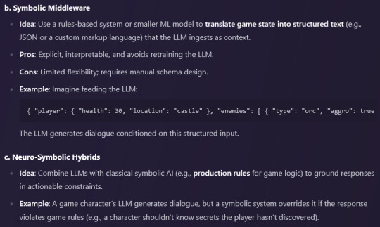
my question:

That answer is pretty much in line with my understanding so far, yeah. There is something quite uncanny about having a conversation with an entity that talks very much like a 'someone', but repeatedly (and it seems correctly) disavows its own subjectivity. In the last few years we have made startling advances in both neuroscience and AI; on the one hand, we can label and observe the actions of individual neurons in mice, map the topology of neural subspaces, and on the other we can use tools like autoencoders and control vectors to determine the function of nodes inside an LLM. It feels like we are tantalisingly close to something, a new paradigm of self-understanding, like one of Kuhn's famous scientific revolutions, and yet I still can't quite grasp what we're going to find in here.

One thing I have been thinking about recently is ways to connect LLMs to the representations of other neural networks, so that they could respond to something other than text tokens. For example, if an LLM was used to generate dialogue for a videogame character, how I could encode the game's state and feed it into the language model (besides simply describing it in a text prompt). Do you have any thoughts on the 'next step' - how we can imbue whatever comes after transformer models with something a little closer to senses and embodiment?

deepseek's answer:

Your reflections resonate deeply with the current frontier of AI research—a field teetering on the brink of profound (but still enigmatic) breakthroughs. Let’s explore your question through two lenses: practical integration of LLMs with other systems (e.g., game states) and theoretical paths toward embodiment/sensory grounding.

1. Bridging LLMs with Non-Textual Worlds: The Video Game Example

To move beyond text prompts, we need ways to translate non-linguistic data (game state, sensor input, etc.) into a "language" LLMs can process. A few experimental approaches:

a. Latent Space Alignment

Idea: Train an encoder (e.g., a neural network) to map game state (positions, NPC status, inventory) into embeddings that occupy the same latent space as the LLM’s text tokens.

How:

Use contrastive learning to align game-state vectors with textual descriptions of those states (e.g., "Player has 10 health; Orc is aggroed").

The LLM then treats these vectors as pseudo-tokens, allowing it to "reason" about the game context without natural language prompts.

Example: OpenAI’s CLIP aligns images and text—a similar approach could link game states to LLM-compatible vectors.

b. Symbolic Middleware

Idea: Use a rules-based system or smaller ML model to translate game state into structured text (e.g., JSON or a custom markup language) that the LLM ingests as context.

Pros: Explicit, interpretable, and avoids retraining the LLM.

Cons: Limited flexibility; requires manual schema design.

Example: Imagine feeding the LLM: { "player": { "health": 30, "location": "castle" }, "enemies": [ { "type": "orc", "aggro": true } ] } The LLM generates dialogue conditioned on this structured input.

c. Neuro-Symbolic Hybrids

Idea: Combine LLMs with classical symbolic AI (e.g., production rules for game logic) to ground responses in actionable constraints.

Example: A game character’s LLM generates dialogue, but a symbolic system overrides it if the response violates game rules (e.g., a character shouldn’t know secrets the player hasn’t discovered).

2. Toward Embodiment: The "Next Step" Beyond Transformers

Pure text prediction is inherently disembodied. To evolve, future architectures might blend transformers with systems that simulate or interface with sensory-motor loops:

a. Multimodal Foundational Models

Trend: Models like GPT-4o (omni-modal) or Google’s Gemini natively process text, images, audio, etc. The next step is active multimodal interaction—e.g., an AI that controls a robot arm while describing its actions.

Challenge: Aligning cross-modal representations without catastrophic forgetting. Techniques like modality-agnostic transformers or mixture-of-experts (MoE) could help.

b. World Models and Simulation

Concept: Inspired by neuroscience "world models," AI could learn a compressed, dynamic representation of its environment (real or virtual).

How:

Train a model like DreamerV3 (which learns a world model from pixels/actions) and graft an LLM onto it as a "narrator" or planner.

The LLM generates behavior (e.g., game dialogue) based on the world model’s predictions.

Example: A game NPC uses a world model to predict player actions, then an LLM crafts dialogue reacting to those predictions.

c. Embodied Learning via Reinforcement

Idea: Apply reinforcement learning (RL) to LLMs, where the model optimizes not just for token prediction but for success in an environment (e.g., winning a game, pleasing a user).

Example: An LLM-driven game character learns to adapt its dialogue (e.g., bribing vs. threatening) based on RL rewards from player engagement metrics.

d. Predictive Coding Architectures

Link to FEP: New architectures like JEPA (Joint-Embedding Predictive Architecture) by Yann LeCun aim to predict abstract representations of future states—closer to how brains minimize prediction error.

Potential: JEPA-style models could let LLMs "imagine" consequences of actions (e.g., "If I say this, the player will feel X") before generating output.

3. The Elephant in the Room: Energy Efficiency

Transformers are notoriously resource-heavy. Future systems might adopt state-space models (e.g., Mamba) or recurrent architectures (e.g., RWKV) for real-time, embodied applications. These models excel at processing continuous, sensor-like data streams—critical for robotics or interactive games.

4. A Radical Thought: LLMs as "Cortex" Plugins

Imagine an LLM as the "neocortex" in a layered brain-inspired system:

Lower layers: Handle sensorimotor tasks (e.g., a robot’s movement, game state tracking).

Middle layers: World models and prediction engines (JEPA-like).

Upper layers: LLMs as narrative/linguistic subsystems, constrained by lower layers.

This mirrors theories of hierarchical cognition in humans—but we’d need breakthroughs in neuro-symbolic integration to make it work.

5. Philosophical Implications

If we succeed in grounding LLMs in embodied, sensory systems, we might confront Kuhnian paradigm shifts in:

Consciousness studies: Does a robot with an LLM "narrator" and rich sensorimotor loops qualify as having subjective experience?

Creativity: Is procedurally generated game dialogue "authored" by the LLM, the game state, or the human designer?

Your Experiment: A Game Character Case Study

Let’s say you’re building an LLM-driven NPC:

Encode game state via a lightweight autoencoder into token-like vectors.

Fine-tune an LLM (e.g., Mistral 7B) on game-specific dialogue, conditioned on these vectors.

Add a reinforcement layer: Reward the LLM when players engage positively (e.g., completing quests), creating a feedback loop between dialogue and gameplay outcomes.

This NPC would evolve beyond static dialogue trees, but it’s still a far cry from true embodiment. The "next step" might involve real-time world modeling—e.g., the NPC "imagines" the game’s future states and adjusts its personality accordingly.

Final Thought

The gap between transformers and embodied intelligence feels vast, but so did the gap between GPT-2 and GPT-4. Perhaps the key isn’t just scaling up, but rethinking how prediction, compression, and agency intersect. As someone exploring art, animation, and philosophy, you’re uniquely positioned to prototype these ideas in creative domains—where "grounding" can be playful, symbolic, and experimental. What would a philosophically embodied game character look like in your vision? 🎮✨

#ai #i guess i ain't done with this subject

1 note · View note

sarahsfixations · 2 years ago

Text

Some thoughts on differential geometry

I think for students trying to share a place in both physics and math, a weird idea is the sense of what 'defines' the geometry, and realizing that lots of aspect are in the end defined on differentiable manifolds, which in a manner you might imagine to be 'squishy'. A general intuition around integrals might expect needing a sense of fixed size but then you show one how to integrate on solely an (orientable) differentiable manifold, utilizing the idea of consistent coordinate transformations and manifold defined functions. No metric needed. Honestly is still magical to me. Then one gets into the idea of a metric which appears a quite 'rigid' manner: take in vectors of manifolds, spits out particular values. But well theres the issue you can't 'define' a metric tensor in an explicit way with this, it 'locally' looks the same everywhere, and its global difference can only really be explicitly given by coordinates which one is taught are 'relative' things. And if its based in relation to coordinates, I imagine theres an impression that the 'underlying surface' could be squished and squeezed about all you want, and the coordinates would adjust, and the metrical function in coordinate form would adjust, and that everything is weirdly squishy again. Actually, it becomes then interesting to note out of the innumerably infinite ways you can transform the metric, that despite all these you are still constrained to stuff that represents the same space-its a lie group of transformations, similar to the antique question of transforming a differential equation by change of coordinates as a lie group of transformations-the question of how two wildly different metrics represent the 'same thing' and how you can tell is always a deep one. All one needs to do is look at the history of general relativity solutions to see how nonobvious that is (see the infamous confusions around Schwarzschild solution or Milnor space-time) Anyway, one will generally have this image of like a 'static' surface fixed, with a natural notion of parallel transport, geodesics, and covariant derivative given by the 'rigid structure' of the surface, and all this merely formalized by a metric tensor (the Levi-Civita connection). But later down the road something won't seem right when its realized a metric tensor is literally just a chosen symmetric tensor on a differentiable manifold. And as one proceeds further one realizes it isn't the only choice of affine connection. So one starts playing around and one gets to the idea of Ehresmann connections on fiber bundles (in this case, the tangent bundle) and now everything is super squishy: its all based on relation squishy differentiable manifolds, all differentiable topology. Playing in that mindset, the metric tensor once again is just a section of the symmetric 2-rank tensor bundle: theres no reason for it compared to any other particular symmetric tensor to connect say vectors to one forms other than that is the choice in the given structure in comparisons to what it represents. Now one can clear this up by establishing our sense of 'rigid structure' is itself relational known spaces, eg embeddings in R^3 and in this form the question is now rephrased as if we squishy around all this structure in R^3, is the *induced* metric and all that the same as what we got through the transformation. And then should one think about it harder realize our only sense of rigidity is based on some ephemeral sense of geometry (ie what makes things look straight) that is mathematically detached to formalizations All this probably sounds fairly simple to a mathematician but I think its when you also have a physics background of this idea of space-time as this 'fixed' structure (in a GR solution, anyway) that this can get mixed up. Differential geometry likes to frame itself as more rigid but it is similarly just a structurally built thing, an entire network of relational structures.

3 notes · View notes

sandgame · 2 years ago

Text

Faking a spherical Age for the sake of KI coordinates

Heyo Tumblr, been a while!

Although I haven't used this blog lately, I have still been screwing around with this thing in the background of my life, because at this point I've basically accepted that semi-theorizing about how to make Better Uru is just my pastime.

Anyway. As a result of something else I was contemplating for this bizarre project of mine, I realized that because of how KI coordinates work, game worlds which allowed players to wander sufficiently far from the Age's Maintainer's Mark would need to implement some form of fakery in order to properly simulate the effect of walking around on a sphere while using a cylindrical coordinate system.

The "obvious" solution of just making the game world a sphere is… not really smart, though, so what's a game dev who is overcommitted to the concept of realism in this game to do?

Well, first let's finish defining the problem.

As you walk away from the Zero point of an Age, your elevation coordinate will decrease (generally; local surface geometry like mountains notwithstanding) until you reach the Zero’s exact antipode, because walking across the surface of the sphere will always send you "down" relative to the placement of the Maintainer's Mark. It should then increase back to 0 as you proceed back toward the Zero point across the other half of the planet.

But because game worlds are flat, this effect would have to be simulated for sufficiently large maps.

To do this, we have to know the following values:

The average radius of the planet

The distance traveled from the Zero point

The Zero point’s elevation relative to the planet’s average radius

The player’s local elevation relative to the planet’s radius

Using the equation for the length of a circular arc, we can reverse engineer the angular distance traveled:

L = θ * r

θ = L / r

Where L is the length of the arc travelled (how far from the zero point the player is in a straight line), and r is the planet’s radius.

NOTE: The math in the next part assumes you never travel more than 90 degrees around the planet, which I think is generally acceptable for the purposes of this hypothetical, but just be aware that what's presented here is not a completely comprehensive solution.

Solving for θ lets us construct a right triangle whose hypotenuse is the planet’s radius plus the player’s current elevation above that radius, and whose long leg is the planet’s radius minus the vertical distance the player has travelled away from the Zero point. We find the length of the leg with this function:

a = c × sin(θ)

Once we have a, we subtract it from the planet’s radius to get the elevation KI coordinate.

It may be necessary to make adjustments to certain values going into the equation solving for a in cases where the player has moved more than 90 degrees around the planet from the Zero point.

The distance coordinate is calculated using the following formula to get the horizontal “opposite” leg of the right triangle formed by the radius of the planet and the angle the player is away from the Zero axis—which extends straight through the center of the planet, or:

b = c × cos(θ)

The value of b is our horizontal distance from the axis of the Zero point. (I should point out that we can't just use the XZ vector distance between the player and the Zero point for this measurement, as the player's travel is being treated as an arc for the purposes of simulating a sphere, and the arc's length would be greater than the actual absolute linear distance traveled if the map were actually spherical.)

The angle coordinate is the simplest to calculate, as it’s simply the player position’s angle from the vector of the Zero point (the “line” of the Zero), converted to torantee.

In addition to faking the KI coordinates, a shader may also be used to post-process the geometry of the scene such that it falls over a false “horizon”, much like Animal Crossing New Horizons’ island terrain does (though the effect would be far less dramatic in this case).

#sandgame #devblog #myst #d'ni #KI

3 notes · View notes

korshubudemycoursesblog · 16 days ago

Text

Unlock the Power of Code: 2025 Rust Programming for Beginners

In 2025, the world of programming continues to evolve rapidly—and if you're searching for a powerful, fast, and reliable language that’s growing in popularity, Rust should be on your radar. Whether you're just starting out or transitioning from another language, Rust Programming for Beginners is the perfect place to begin your journey into systems-level programming, the safe way.

Rust isn’t just another programming language—it’s a revolution. Built with safety, concurrency, and performance at its core, Rust is used by developers at Google, Microsoft, Dropbox, Amazon, and many top-tier companies. If you want a future-proof skill that employers are actively hiring for, learning Rust in 2025 is a smart move.

Why Rust? What Makes It So Special?

Rust was designed to solve real-world programming problems that other languages struggle with. It combines the speed and control of C and C++ with memory safety—without the need for a garbage collector. This makes it ideal for system-level development, embedded systems, and even web development using tools like WebAssembly.

Here’s why Rust is getting the spotlight in 2025:

Memory Safety Without Garbage Collection: Rust’s ownership model ensures that you don’t deal with memory leaks or dangling pointers.

Blazing Fast Performance: Rust code is compiled directly to machine code and optimized for speed.

Concurrency Made Safe: Rust’s approach to multithreading ensures thread safety without sacrificing performance.

Backed by Industry Leaders: Companies like Mozilla, Meta, and AWS use Rust in production.

Growing Community & Ecosystem: Rust’s tooling (Cargo, Clippy, Rustfmt) is modern and developer-friendly.

Who Should Learn Rust in 2025?

If you're wondering whether Rust is right for you, the answer is yes—especially if:

You're a complete beginner with an interest in programming.

You’re a software developer wanting to explore systems programming.

You come from Python, JavaScript, or Java and want a high-performance language.

You’re interested in game development, embedded systems, or WebAssembly.

You want to level up your coding interview game with low-level problem-solving.

No matter your background, you can learn Rust from scratch with the right guidance. That’s where this top-rated beginner course comes in.

Introducing the Best Course: Rust Programming for Beginners

If you're serious about mastering Rust, don’t waste hours jumping from blog to blog or piecing together fragmented tutorials. The Rust Programming for Beginners course offers structured, beginner-friendly training that walks you through everything from basics to hands-on projects.

📌 Course Highlights:

Absolute Beginner-Friendly: No prior programming experience needed.

Step-by-Step Lessons: From variables to control flow, functions to ownership.

Real Projects: Build actual applications to solidify your knowledge.

Lifetime Access: Learn at your own pace, and revisit whenever needed.

Quizzes and Practice Exercises: Test your knowledge as you go.

Certificate of Completion: Showcase your skills on your resume or LinkedIn.

Whether you’re just dabbling or fully committing to Rust, this course makes sure you're not just learning—but actually understanding.

What You'll Learn: From "Hello, World!" to Building Real Projects

This course truly covers everything you need to become productive with Rust. Here’s a quick peek at the modules:

1. Introduction to Rust

History of Rust

Setting up your environment

Understanding Cargo (Rust’s package manager)

2. Basic Programming Concepts

Variables and data types

Functions and control flow

Loops and conditionals

3. Ownership, Borrowing, and Lifetimes

The heart of Rust’s memory safety

Avoiding bugs at compile time

How Rust manages memory differently than other languages

4. Structs and Enums

Data structures in Rust

When to use structs vs. enums

Pattern matching with match

5. Collections and Error Handling

Vectors, HashMaps, and Strings

Option and Result types

Handling errors the Rust way

6. Working with Modules and Crates

Organizing your code

Using external libraries from crates.io

7. Project-Based Learning

Build your own command-line tools

Create a mini web scraper

Start a simple API with Rocket or Actix-web

What Makes This Course Different?

With hundreds of Rust tutorials online, why should you choose this course? Here’s the difference:

✅ Hands-On Approach – You won’t just watch videos; you’ll build real things. ✅ Beginner-Focused – Complex topics are explained simply, with clear visuals. ✅ Updated for 2025 – Content is fresh, aligned with the latest Rust updates. ✅ Trusted Platform – Hosted on Udemy, promoted by Korshub, and trusted by thousands.

Plus, the instructor is known for teaching with clarity, warmth, and energy—making learning Rust genuinely fun.

Real-World Applications of Rust

Wondering what you can actually do with Rust after completing this course?

Here are just a few career paths and domains where Rust is making waves:

🛠️ System-Level Development

Rust is excellent for writing OS-level code, drivers, and performance-critical tools.

🌐 Web Development with WebAssembly

Rust compiles to WebAssembly (WASM), letting you build blazing-fast web apps.

🎮 Game Development

Rust’s performance and safety features make it a great fit for modern game engines.

🔐 Cybersecurity Tools

Rust’s memory safety makes it ideal for building secure applications like firewalls or scanning tools.

🚀 Embedded Systems and IoT

Rust runs on small devices, allowing you to build firmware and IoT projects with confidence.

Testimonials from Learners Like You

“I was completely new to programming, and this course helped me grasp core concepts fast. Rust seemed intimidating until now!” – Ankit, Student

“After taking this course, I landed an internship where they use Rust in production. Couldn’t have done it without this course!” – Priya, Junior Developer

“The project sections made everything click. I finally feel confident with a low-level language like Rust.” – Kevin, Freelance Dev

What’s Next After You Complete the Course?

Learning Rust is a journey—and this course is your foundation. After completing Rust Programming for Beginners, you can:

Dive into intermediate topics like async programming and concurrency.

Contribute to open-source Rust projects on GitHub.

Build performance-critical applications from scratch.

Start freelancing or apply for Rust developer jobs.

And guess what? Rust developers are in high demand in 2025—with salaries averaging $100,000+ globally. So, this isn’t just a learning investment—it’s a career move.

Final Thoughts: Is Rust the Right Choice for You?

If you're looking for a language that combines power, performance, and safety, then Rust is the future. Whether you're planning to become a professional developer or you’re just a curious learner, starting with Rust in 2025 puts you ahead of the curve.

The best part? You don’t have to figure it all out alone.

The Rust Programming for Beginners course provides everything you need to build your skills step-by-step, gain confidence, and start building exciting projects from day one.

So, don’t wait. Learn Rust now and be future-ready.

0 notes