#DFS Algorithm for Connected Graph

[justnshalom]

Connected Sum Solution for Hackerrank

Problem Statement Given a graph with n nodes and m edges, we need to find the sum of the sizes of connected components in the graph. Each connected component is a subgraph in which every pair of nodes is connected by a path. For example, consider the following graph: 1 - 2 | 3 - 4 | 5 - 6 In this graph, there are 3 connected components: {1, 2}, {3, 4}, and {5, 6}. The sizes of these connected…

[govindhtech]

4DBInfer: A Tool for Graph-Based Prediction in Databases

4DBInfer

A database-based graph-centric predictive modelling benchmark.

4DBInfer enables model comparison, prediction tasks, database-to-graph extraction, and graph-based predictive architectures.

4DBInfer, an extensive open-source benchmarking toolbox, focusses on graph-centric predictive modelling on Relational Databases (RDBs). Shanghai Lablet of Amazon built it to meet the major gap in well-established, publically accessible RDB standards for training and assessment.

As computer vision and natural language processing advance, predictive machine learning models using RDBs lag behind. The lack of public RDB benchmarks contributes to this gap. Single-table or graph datasets from preprocessed relational data often form the basis for RDB prediction models. RDBs' natural multi-table structure and properties are not fully represented by these methods, which may limit model performance.

4DBInfer addresses this with a 4D exploring framework. The 4-D design of RDB predictive analytics allows for deep exploration of the model design space and meticulous comparison of baseline models along these four critical dimensions:

4DBInfer includes RDB benchmarks from social networks, advertising, and e-commerce. Temporal evolution, schema complexity, and scale (billions of rows) vary among these datasets.

For every dataset, 4DBInfer finds realistic prediction tasks, such as estimating missing cell values.

Techniques for RDB-to-graph extraction: The program supports many approaches to retain the rich tabular information of big RDBs' structured data while transforming it into graph representations. The Row2Node function turns every table row into a graph node with foreign-key edges, whereas the Row2N/E method turns some rows into edges only to capture more sophisticated relational patterns. Additionally, “dummy tables” improve graph connectivity. According to the text, these algorithms subsample well.

FourDBInfer implements several resilient baseline structures for graph-based learning. These cover early and late feature-fusion paradigms. Deep Feature Synthesis (DFS) models collect tabular data from the graph before applying typical machine learning predictors, while Graph Neural Networks (GNNs) train node embeddings using relational message passing. These trainable models output subgraph-based predictions with well-matched inductive biases.

Comprehensive 4DBInfer tests yielded many noteworthy findings:

Graph-based models that use the complete multi-table RDB structure usually perform better than single-table or table joining models. This shows the value of RDB relational data.

The RDB-to-graph extraction strategy considerably affects model performance, emphasising the importance of design space experimentation.

GNNs and other early feature fusion graph models perform better than late-fusion models. Late-fusion models can compete, especially with computing limits.

Model performance depends on the job and dataset, underscoring the need for many benchmarks to provide correct findings.

The results suggest a future research topic: the tabular-graph machine learning paradigm nexus may yield the best solutions.

4DBInfer provides a consistent, open-sourced framework for the community to develop creative approaches that accelerate relational data prediction research. The source code of 4DBInfer is public.

[adayiniilm]

Data Structures and Algorithms: The Building Blocks of Efficient Programming

The world of programming is vast and complex, but at its core, it boils down to solving problems using well-defined instructions.  While the specific code varies depending on the language and the task, the fundamental principles of data structures and algorithms underpin every successful application.  This blog post delves into these crucial elements, explaining their importance and providing a starting point for understanding and applying them.

What are Data Structures and Algorithms?

Imagine you have a vast collection of books.  You could haphazardly pile them, making it nearly impossible to find a specific title.  Alternatively, you could organize them by author, genre, or subject, with indexed catalogs, allowing quick retrieval. Data structures are the organizational systems for data. They define how data is stored, accessed, and manipulated.

Algorithms, on the other hand, are the specific instructions—the step-by-step procedures—for performing tasks on the data within the chosen structure.  They determine how to find a book, sort the collection, or even search for a particular keyword within all the books.

Essentially, data structures provide the containers, and algorithms provide the methods to work with those containers efficiently.

Fundamental Data Structures:

Arrays:  A contiguous block of memory used to store elements of the same data type.  Accessing an element is straightforward using its index (position).  Arrays are efficient for storing and accessing data, but inserting or deleting elements can be costly.  Think of a numbered list of items in a shopping cart.

Linked Lists: A linear data structure where elements are not stored contiguously. Instead, each element (node) contains data and a pointer to the next node. This allows for dynamic insertion and deletion of elements but accessing a specific element requires traversing the list from the beginning.  Imagine a chain where each link has a piece of data and points to the next link.

Stacks:  A LIFO (Last-In, First-Out) structure. Think of a stack of plates: the last plate placed on top is the first one removed.  Stacks are commonly used for function calls, undo/redo operations, and expression evaluation.

Queues: A FIFO (First-In, First-Out) structure.  Imagine a queue at a ticket counter—the first person in line is the first one served. Queues are useful for managing tasks, processing requests, and implementing breadth-first search algorithms.

Trees:Hierarchical data structures that resemble a tree with a root, branches, and leaves.  Binary trees, where each node has at most two children, are common for searching and sorting.  Think of a file system's directory structure, representing files and folders in a hierarchical way.

Graphs:  A collection of nodes (vertices) connected by edges.  Represent relationships between entities. Examples include social networks, road maps, and dependency diagrams.

Crucial Algorithms:

Sorting Algorithms:  Bubble Sort, Insertion Sort, Merge Sort, Quick Sort, Heap Sort—these algorithms arrange data in ascending or descending order.  Choosing the right algorithm for a given dataset is critical for efficiency.  Large datasets often benefit from algorithms with time complexities better than O(n^2).

Searching Algorithms:  Linear Search, Binary Search—finding a specific item in a dataset.  Binary search significantly improves efficiency on sorted data compared to linear search.

Graph Traversal Algorithms:  Depth-First Search (DFS), Breadth-First Search (BFS)—exploring nodes in a graph.  Crucial for finding paths, determining connectivity, and solving various graph-related problems.

Hashing:  Hashing functions take input data and produce a hash code used for fast data retrieval. Essential for dictionaries, caches, and hash tables.

Why Data Structures and Algorithms Matter:

Efficiency:  Choosing the right data structure and algorithm is crucial for performance.  An algorithm's time complexity (e.g., O(n), O(log n), O(n^2)) significantly impacts execution time, particularly with large datasets.

Scalability:Applications need to handle growing amounts of data.  Well-designed data structures and algorithms ensure that the application performs efficiently as the data size increases.

Readability and Maintainability:  A structured approach to data handling makes code easier to understand, debug, and maintain.

Problem Solving:  Understanding data structures and algorithms helps to approach problems systematically, breaking them down into solvable sub-problems and designing efficient solutions.

[leetcode1]

leetcode 200 : number of islands : python

LeetCode problem 200, "Number of Islands," involves finding and counting isolated groups of connected 1s in a 2D grid of 0s and 1s, where 1 represents land and 0 represents water. The task is to identify each "island," where an island is a group of adjacent lands connected horizontally or vertically. This problem is commonly solved using Depth-First Search (DFS) or Breadth-First Search (BFS) to explore and mark connected cells as visited. The problem challenges you to understand graph traversal and apply search algorithms effectively in grid-based representations, with an optimal time complexity of O(m * n).

[nocodehackathon]

Essential Algorithms and Data Structures for Competitive Programming

Competitive programming is a thrilling and intellectually stimulating field that challenges participants to solve complex problems efficiently and effectively. At its core, competitive programming revolves around algorithms and data structures—tools that help you tackle problems with precision and speed. If you're preparing for a competitive programming contest or just want to enhance your problem-solving skills, understanding essential algorithms and data structures is crucial. In this blog, we’ll walk through some of the most important ones you should be familiar with.

1. Arrays and Strings

Arrays are fundamental data structures that store elements in a contiguous block of memory. They allow for efficient access to elements via indexing and are often the first data structure you encounter in competitive programming.

Operations: Basic operations include traversal, insertion, deletion, and searching. Understanding how to manipulate arrays efficiently can help solve a wide range of problems.

Strings are arrays of characters and are often used to solve problems involving text processing. Basic string operations like concatenation, substring search, and pattern matching are essential.

2. Linked Lists

A linked list is a data structure where elements (nodes) are stored in separate memory locations and linked together using pointers. There are several types of linked lists:

Singly Linked List: Each node points to the next node.

Doubly Linked List: Each node points to both the next and previous nodes.

Circular Linked List: The last node points back to the first node.

Linked lists are useful when you need to frequently insert or delete elements as they allow for efficient manipulation of the data.

3. Stacks and Queues

Stacks and queues are abstract data types that operate on a last-in-first-out (LIFO) and first-in-first-out (FIFO) principle, respectively.

Stacks: Useful for problems involving backtracking or nested structures (e.g., parsing expressions).

Queues: Useful for problems involving scheduling or buffering (e.g., breadth-first search).

Both can be implemented using arrays or linked lists and are foundational for many algorithms.

4. Hashing

Hashing involves using a hash function to convert keys into indices in a hash table. This allows for efficient data retrieval and insertion.

Hash Tables: Hash tables provide average-case constant time complexity for search, insert, and delete operations.

Collisions: Handling collisions (when two keys hash to the same index) using techniques like chaining or open addressing is crucial for effective hashing.

5. Trees

Trees are hierarchical data structures with a root node and child nodes. They are used to represent hierarchical relationships and are key to many algorithms.

Binary Trees: Each node has at most two children. They are used in various applications such as binary search trees (BSTs), where the left child is less than the parent, and the right child is greater.

Binary Search Trees (BSTs): Useful for dynamic sets where elements need to be ordered. Operations like insertion, deletion, and search have an average-case time complexity of O(log n).

Balanced Trees: Trees like AVL trees and Red-Black trees maintain balance to ensure O(log n) time complexity for operations.

6. Heaps

A heap is a specialized tree-based data structure that satisfies the heap property:

Max-Heap: The value of each node is greater than or equal to the values of its children.

Min-Heap: The value of each node is less than or equal to the values of its children.

Heaps are used in algorithms like heap sort and are also crucial for implementing priority queues.

7. Graphs

Graphs represent relationships between entities using nodes (vertices) and edges. They are essential for solving problems involving networks, paths, and connectivity.

Graph Traversal: Algorithms like Breadth-First Search (BFS) and Depth-First Search (DFS) are used to explore nodes and edges in graphs.

Shortest Path: Algorithms such as Dijkstra’s and Floyd-Warshall help find the shortest path between nodes.

Minimum Spanning Tree: Algorithms like Kruskal’s and Prim’s are used to find the minimum spanning tree in a graph.

8. Dynamic Programming

Dynamic Programming (DP) is a method for solving problems by breaking them down into simpler subproblems and storing the results of these subproblems to avoid redundant computations.

Memoization: Storing results of subproblems to avoid recomputation.

Tabulation: Building a table of results iteratively, bottom-up.

DP is especially useful for optimization problems, such as finding the shortest path, longest common subsequence, or knapsack problem.

9. Greedy Algorithms

Greedy Algorithms make a series of choices, each of which looks best at the moment, with the hope that these local choices will lead to a global optimum.

Applications: Commonly used for problems like activity selection, Huffman coding, and coin change.

10. Graph Algorithms

Understanding graph algorithms is crucial for competitive programming:

Shortest Path Algorithms: Dijkstra’s Algorithm, Bellman-Ford Algorithm.

Minimum Spanning Tree Algorithms: Kruskal’s Algorithm, Prim’s Algorithm.

Network Flow Algorithms: Ford-Fulkerson Algorithm, Edmonds-Karp Algorithm.

Preparing for Competitive Programming: Summer Internship Program

If you're eager to dive deeper into these algorithms and data structures, participating in a summer internship program focused on Data Structures and Algorithms (DSA) can be incredibly beneficial. At our Summer Internship Program, we provide hands-on experience and mentorship to help you master these crucial skills. This program is designed for aspiring programmers who want to enhance their competitive programming abilities and prepare for real-world challenges.

What to Expect:

Hands-On Projects: Work on real-world problems and implement algorithms and data structures.

Mentorship: Receive guidance from experienced professionals in the field.

Workshops and Seminars: Participate in workshops that cover advanced topics and techniques.

Networking Opportunities: Connect with peers and industry experts to expand your professional network.

By participating in our DSA Internship, you’ll gain practical experience and insights that will significantly boost your competitive programming skills and prepare you for success in contests and future career opportunities.

In conclusion, mastering essential algorithms and data structures is key to excelling in competitive programming. By understanding and practicing these concepts, you can tackle complex problems with confidence and efficiency. Whether you’re just starting out or looking to sharpen your skills, focusing on these fundamentals will set you on the path to success.

Ready to take your skills to the next level? Join our Summer Internship Program and dive into the world of algorithms and data structures with expert guidance and hands-on experience. Your journey to becoming a competitive programming expert starts here!

[mazhaipilipiri]

include <iostream>

using namespace std;

class node{

public:

node* next;

int val;

node(int k){

val=k;

next=NULL;

}

class q{

public:

node* head;

node* tail;

q(){

head=NULL;

tail=NULL;

}

push(int k){

if (q->head==NULL){

q->head=k;

q->tail=k;

#include <iostream>

#include <algorithm>

#include <vector>

#include <queue>

#include <climits>

using namespace std;

class graph{

int v;

vector<vector<int>> a;

graph(int vertex):v(vertex),a(vertex){}

void insert_edge(int u,int v){

a[u].push_back(v);

a[v].push_back(u);

}

void dfs(int s,vector<bool>& vis){

vector<bool> visited(v,false);

vector<int> st;

visited[s]=true;

st.push_back(s);

while(!st.empty()){

int c=st.back();

st.pop_back();

cout<<c<<" ";

for(int n:a[c]){

if(!visited[n]){

visited[n]=true;

st.push_back(n);

}

}

}

}

void bfs(int s){

vector<bool> visited(v,false);

queue<int> q;

visited[s]=true;

q.push(s);

while(!q.empty()){

int c=q.front();

q.pop();

cout<<c<<" ";

for(int n:a[c]){

if(!visited[n]){

visited[n]=true;

q.push(n);

}

}

}

}

bool connected(){

vector<bool> visited(v,false);

dfs(0,visited);

for(bool vi:visited){

if(!v){

return false;

}

}

return true;

}

bool directed(){

for(int i=0;i<v;i++){

for(int j:a[i]){

if(find(a[j].begin(),a[j].end(),i)==a[j].end()){

return true;

}

}

}

return false;

}

};

[myprogrammingsolver]

Assignment 9 - Graph

OBJECTIVES Applications of DF Traversal Dijkstra’s algorithm Overview In this assignment, you will apply DF traversal for finding connected cities in a graph and find the shortest path using Dijkstra’s algorithm. Graph Class Your code should implement graph traversal for cities. A header file that lays out this graph can be found in ​Graph.hpp​on Moodle. ​As usual, do not modify the header…

[tutort-academy]

How to Ace Your DSA Interview, Even If You're a Newbie

Are you aiming to crack DSA interviews and land your dream job as a software engineer or developer? Look no further! This comprehensive guide will provide you with all the necessary tips and insights to ace your DSA interviews. We'll explore the important DSA topics to study, share valuable preparation tips, and even introduce you to Tutort Academy DSA courses to help you get started on your journey. So let's dive in!

Why is DSA Important?

Before we delve into the specifics of DSA interviews, let's first understand why data structures and algorithms are crucial for software development. DSA plays a vital role in optimizing software components, enabling efficient data storage and processing.

From logging into your Facebook account to finding the shortest route on Google Maps, DSA is at work in various applications we use every day. Mastering DSA allows you to solve complex problems, optimize code performance, and design efficient software systems.

Important DSA Topics to Study

To excel in DSA interviews, it's essential to have a strong foundation in key topics. Here are some important DSA topics you should study:

1. Arrays and Strings

Arrays and strings are fundamental data structures in programming. Understanding array manipulation, string operations, and common algorithms like sorting and searching is crucial for solving coding problems.

2. Linked Lists

Linked lists are linear data structures that consist of nodes linked together. It's important to understand concepts like singly linked lists, doubly linked lists, and circular linked lists, as well as operations like insertion, deletion, and traversal.

3. Stacks and Queues

Stacks and queues are abstract data types that follow specific orderings. Mastering concepts like LIFO (Last In, First Out) for stacks and FIFO (First In, First Out) for queues is essential. Additionally, learn about their applications in real-life scenarios.

4. Trees and Binary Trees

Trees are hierarchical data structures with nodes connected by edges. Understanding binary trees, binary search trees, and traversal algorithms like preorder, inorder, and postorder is crucial. Additionally, explore advanced concepts like AVL trees and red-black trees.

5. Graphs

Graphs are non-linear data structures consisting of nodes (vertices) and edges. Familiarize yourself with graph representations, traversal algorithms like BFS (Breadth-First Search) and DFS (Depth-First Search), and graph algorithms such as Dijkstra's algorithm and Kruskal's algorithm.

6. Sorting and Searching Algorithms

Understanding various sorting algorithms like bubble sort, selection sort, insertion sort, merge sort, and quicksort is essential. Additionally, familiarize yourself with searching algorithms like linear search, binary search, and hash-based searching.

7. Dynamic Programming

Dynamic programming involves breaking down a complex problem into smaller overlapping subproblems and solving them individually. Mastering this technique allows you to solve optimization problems efficiently.

These are just a few of the important DSA topics to study. It's crucial to have a solid understanding of these concepts and their applications to perform well in DSA interviews.

Tips to Follow While Preparing for DSA Interviews

Preparing for DSA interviews can be challenging, but with the right approach, you can maximize your chances of success. Here are some tips to keep in mind:

1. Understand the Fundamentals

Before diving into complex algorithms, ensure you have a strong grasp of the fundamentals. Familiarize yourself with basic data structures, common algorithms, and time and space complexities.

2. Practice Regularly

Consistent practice is key to mastering DSA. Solve a wide range of coding problems, participate in coding challenges, and implement algorithms from scratch. Leverage online coding platforms like LeetCode, HackerRank to practice and improve your problem-solving skills.

3. Analyze and Optimize

After solving a problem, analyze your solution and look for areas of improvement. Optimize your code for better time and space complexities. This demonstrates your ability to write efficient and scalable code.

4. Collaborate and Learn from Others

Engage with the coding community, join study groups, and participate in online forums. Collaborating with others allows you to learn different approaches, gain insights, and improve your problem-solving skills.

5. Mock Interviews and Feedback

Simulate real interview scenarios by participating in mock interviews. Seek feedback from experienced professionals or mentors who can provide valuable insights into your strengths and areas for improvement.

Following these tips will help you build a solid foundation in DSA and boost your confidence for interviews.

Conclusion

Mastering DSA is crucial for acing coding interviews and securing your dream job as a software engineer or developer. By studying important DSA topics, following effective preparation tips, and leveraging Tutort Academy's DSA courses, you'll be well-equipped to tackle DSA interviews with confidence. Remember to practice regularly, seek feedback, and stay curious.

Good luck on your DSA journey!

[codezclub]

C Program to implement DFS Algorithm for Connected Graph

DFS Algorithm for Connected Graph Write a C Program to implement DFS Algorithm for Connected Graph. Here’s simple Program for traversing a directed graph through Depth First Search(DFS),  visiting only those vertices that are reachable from start vertex. Depth First Search (DFS) Depth First Search (DFS) algorithm traverses a graph in a depthward motion and uses a stack to remember to get the next…

[programmingsolver]

Assignment 9 - Graph

  OBJECTIVES   Applications of DF Traversal   Dijkstra’s algorithm   Overview   In this assignment, you will apply DF traversal for finding connected cities in a graph and find the shortest path using Dijkstra’s algorithm.   Graph Class   Your code should implement graph traversal for cities. A header file that lays out this graph can be found in ​Graph.hpp​on Moodle. ​As usual, do not modify…

[hi-tech-multiplex]

DFS Trees

You are given a connected undirected graph consisting of nn vertices and mm edges. The weight of the ii-th edge is ii. Here is a wrong algorithm of finding a minimum spanning tree (MST) of a graph: vis := an array of length ns := a set of edgesfunction dfs(u): vis[u] := true iterate through each edge (u, v) in the order from smallest to largest edge weight if vis[v] = false add edge (u, v) into…

[holytheoristtastemaker]

Have you ever solved a real-life maze? The approach that most of us take while solving a maze is that we follow a path until we reach a dead end, and then backtrack and retrace our steps to find another possible path. This is exactly the analogy of Depth First Search (DFS). It's a popular graph traversal algorithm that starts at the root node, and travels as far as it can down a given branch, then backtracks until it finds another unexplored path to explore. This approach is continued until all the nodes of the graph have been visited. In today’s tutorial, we are going to discover a DFS pattern that will be used to solve some of the important tree and graph questions for your next Tech Giant Interview! We will solve some Medium and Hard Leetcode problems using the same common technique. So, let’s get started, shall we?

Implementation

Since DFS has a recursive nature, it can be implemented using a stack. DFS Magic Spell:

Push a node to the stack

Pop the node

Retrieve unvisited neighbors of the removed node, push them to stack

Repeat steps 1, 2, and 3 as long as the stack is not empty

Graph Traversals

In general, there are 3 basic DFS traversals for binary trees:

Pre Order: Root, Left, Right OR Root, Right, Left

Post Order: Left, Right, Root OR Right, Left, Root

In order: Left, Root, Right OR Right, Root, Left

144.  Binary Tree Preorder Traversal (Difficulty: Medium)

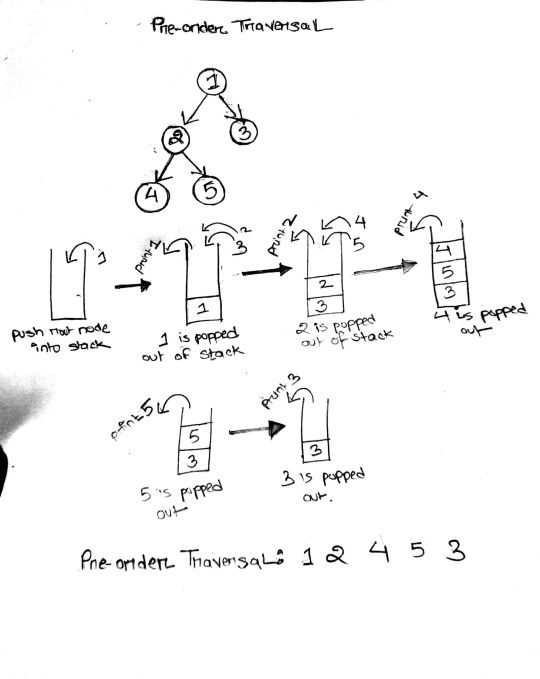
To solve this question all we need to do is simply recall our magic spell. Let's understand the simulation really well since this is the basic template we will be using to solve the rest of the problems.

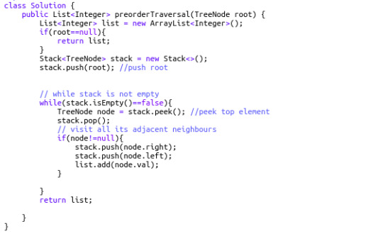
At first, we push the root node into the stack. While the stack is not empty, we pop it, and push its right and left child into the stack. As we pop the root node, we immediately put it into our result list. Thus, the first element in the result list is the root (hence the name, Pre-order). The next element to be popped from the stack will be the top element of the stack right now: the left child of root node. The process is continued in a similar manner until the whole graph has been traversed and all the node values of the binary tree enter into the resulting list.

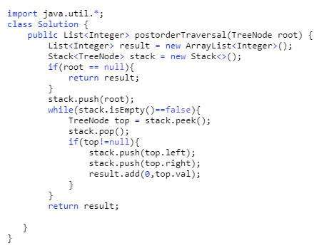
145. Binary Tree Postorder Traversal (Difficulty: Hard)

Pre-order traversal is root-left-right, and post-order is right-left-root. This means post order traversal is exactly the reverse of pre-order traversal. So one solution that might come to mind right now is simply reversing the resulting array of pre-order traversal. But think about it – that would cost O(n) time complexity to reverse it. A smarter solution is to copy and paste the exact code of the pre-order traversal, but put the result at the top of the linked list (index 0) at each iteration. It takes constant time to add an element to the head of a linked list. Cool, right?

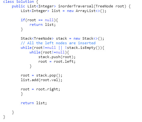
94. Binary Tree Inorder Traversal (Difficulty: Medium)

Our approach to solve this problem is similar to the previous problems. But here, we will visit everything on the left side of a node, print the node, and then visit everything on the right side of the node.

323. Number of Connected Components in an Undirected Graph (Difficulty: Medium)

Our approach here is to create a variable called ans that stores the number of connected components. First, we will initialize all vertices as unvisited. We will start from a node, and while carrying out DFS on that node (of course, using our magic spell), it will mark all the nodes connected to it as visited. The value of ans will be incremented by 1.

import java.util.ArrayList; import java.util.List; import java.util.Stack; public class NumberOfConnectedComponents { public static void main(String[] args){ int[][] edge = {{0,1}, {1,2},{3,4}}; int n = 5; System.out.println(connectedcount(n, edge)); } public static int connectedcount(int n, int[][] edges) { boolean[] visited = new boolean[n]; List[] adj = new List[n]; for(int i=0; i<adj.length; i++){ adj[i] = new ArrayList<Integer>(); } // create the adjacency list for(int[] e: edges){ int from = e[0]; int to = e[1]; adj[from].add(to); adj[to].add(from); } Stack<Integer> stack = new Stack<>(); int ans = 0; // ans = count of how many times DFS is carried out // this for loop through the entire graph for(int i = 0; i < n; i++){ // if a node is not visited if(!visited[i]){ ans++; //push it in the stack stack.push(i); while(!stack.empty()) { int current = stack.peek(); stack.pop(); //pop the node visited[current] = true; // mark the node as visited List<Integer> list1 = adj[current]; // push the connected components of the current node into stack for (int neighbours:list1) { if (!visited[neighbours]) { stack.push(neighbours); } } } } } return ans; } }

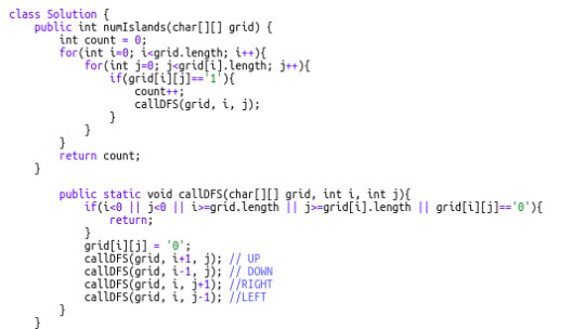
200. Number of Islands (Difficulty: Medium)

This falls under a general category of problems where we have to find the number of connected components, but the details are a bit tweaked. Instinctually, you might think that once we find a “1” we initiate a new component. We do a DFS from that cell in all 4 directions (up, down, right, left) and reach all 1’s connected to that cell. All these 1's connected to each other belong to the same group, and thus, our value of count is incremented by 1. We mark these cells of 1's as visited and move on to count other connected components.

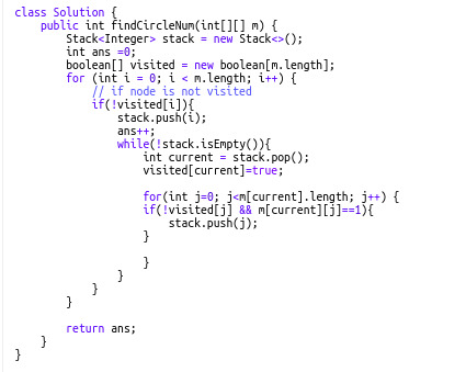
547. Friend Circles (Difficulty: Medium)

This also follows the same concept as finding the number of connected components. In this question, we have an NxN matrix but only N friends in total. Edges are directly given via the cells so we have to traverse a row to get the neighbors for a specific "friend". Notice that here, we use the same stack pattern as our previous problems.

That's all for today! I hope this has helped you understand DFS better and that you have enjoyed the tutorial. Please recommend this post if you think it may be useful for someone else!

[felord]

CSCI 2270 Homework9 -implement graph traversal for cities Solved

CSCI 2270 Homework9 -implement graph traversal for cities Solved

Overview

In this assignment, you will apply DF traversal for finding connected cities in a graph and find the shortest path using Dijkstra’s algorithm.

Graph Class

Your code should implement graph traversal for cities. A header file that lays out this graph can be found in ​Graph.hpp​ on Moodle. ​As usual, do not modify the header file. You may implement helper functions in your .cpp file if you…

[myfreecourses]

Advanced Algorithms In Java

Advanced Algorithms In Java

Graph algorithms, breadth-first search, depth-first search, shortest path, arbitrage, strongly connected components What you’ll learn

Learn about the applications of data structures

Implement advanced algorithms efficiently

Able to move towards advanced topics such as machine learning or big data analysis

Get a good grasp of algorithmic thinking

Get to know graph algorithms: BFS, DFS,…

[shreyauzumaki]

Kosaraju’s Algorithm

Read about the algo in the title, Kosaraju. Works to find Strongly Connected Components in a directed graph in O(V+E) time. 

Core principle - DFS of a graph leads to a tree. Starting from the source and ending at leaf nodes. Do DFS of the graph choosing one as source vertex, and push in stack correspondingly. Higher the node lies in the tree, more the connectivity, hence avoiding the chance for a smaller SCC before a bigger one. Reverse all edges of the graph, pop the stack and do DFS with each popped vertex, repeat this till stack gets over or every node present gets visited. Reversed DFS is the biggest SCC corresponding to the vertex. 

[theresawelchy]

How to Reduce Overfitting in Deep Neural Networks Using Weight Constraints in Keras

Weight constraints provide an approach to reduce the overfitting of a deep learning neural network model on the training data and improve the performance of the model on new data, such as the holdout test set.

There are multiple types of weight constraints, such as maximum and unit vector norms, and some require a hyperparameter that must be configured.

In this tutorial, you will discover the Keras API for adding weight constraints to deep learning neural network models to reduce overfitting.

After completing this tutorial, you will know:

How to create vector norm constraints using the Keras API.

How to add weight constraints to MLP, CNN, and RNN layers using the Keras API.

How to reduce overfitting by adding a weight constraint to an existing model.

Let’s get started.

How to Reduce Overfitting in Deep Neural Networks With Weight Constraints in Keras Photo by Ian Sane, some rights reserved.

Tutorial Overview

This tutorial is divided into three parts; they are:

Weight Constraints in Keras

Weight Constraints on Layers

Weight Constraint Case Study

Weight Constraints in Keras

The Keras API supports weight constraints.

The constraints are specified per-layer, but applied and enforced per-node within the layer.

Using a constraint generally involves setting the kernel_constraint argument on the layer for the input weights and the bias_constraint for the bias weights.

Generally, weight constraints are not used on the bias weights.

A suite of different vector norms can be used as constraints, provided as classes in the keras.constraints module. They are:

Maximum norm (max_norm), to force weights to have a magnitude at or below a given limit.

Non-negative norm (non_neg), to force weights to have a positive magnitude.

Unit norm (unit_norm), to force weights to have a magnitude of 1.0.

Min-Max norm (min_max_norm), to force weights to have a magnitude between a range.

For example, a constraint can imported and instantiated:

# import norm from keras.constraints import max_norm # instantiate norm norm = max_norm(3.0)

Weight Constraints on Layers

The weight norms can be used with most layers in Keras.

In this section, we will look at some common examples.

MLP Weight Constraint

The example below sets a maximum norm weight constraint on a Dense fully connected layer.

# example of max norm on a dense layer from keras.layers import Dense from keras.constraints import max_norm ... model.add(Dense(32, kernel_constraint=max_norm(3), bias_constraint==max_norm(3))) ...

CNN Weight Constraint

The example below sets a maximum norm weight constraint on a convolutional layer.

# example of max norm on a cnn layer from keras.layers import Conv2D from keras.constraints import max_norm ... model.add(Conv2D(32, (3,3), kernel_constraint=max_norm(3), bias_constraint==max_norm(3))) ...

RNN Weight Constraint

Unlike other layer types, recurrent neural networks allow you to set a weight constraint on both the input weights and bias, as well as the recurrent input weights.

The constraint for the recurrent weights is set via the recurrent_constraint argument to the layer.

The example below sets a maximum norm weight constraint on an LSTM layer.

# example of max norm on an lstm layer from keras.layers import LSTM from keras.constraints import max_norm ... model.add(LSTM(32, kernel_constraint=max_norm(3), recurrent_constraint=max_norm(3), bias_constraint==max_norm(3))) ...

Now that we know how to use the weight constraint API, let’s look at a worked example.

Weight Constraint Case Study

In this section, we will demonstrate how to use weight constraints to reduce overfitting of an MLP on a simple binary classification problem.

This example provides a template for applying weight constraints to your own neural network for classification and regression problems.

Binary Classification Problem

We will use a standard binary classification problem that defines two semi-circles of observations, one semi-circle for each class.

Each observation has two input variables with the same scale and a class output value of either 0 or 1. This dataset is called the “moons” dataset because of the shape of the observations in each class when plotted.

We can use the make_moons() function to generate observations from this problem. We will add noise to the data and seed the random number generator so that the same samples are generated each time the code is run.

# generate 2d classification dataset X, y = make_moons(n_samples=100, noise=0.2, random_state=1)

We can plot the dataset where the two variables are taken as x and y coordinates on a graph and the class value is taken as the color of the observation.

The complete example of generating the dataset and plotting it is listed below.

# generate two moons dataset from sklearn.datasets import make_moons from matplotlib import pyplot from pandas import DataFrame # generate 2d classification dataset X, y = make_moons(n_samples=100, noise=0.2, random_state=1) # scatter plot, dots colored by class value df = DataFrame(dict(x=X[:,0], y=X[:,1], label=y)) colors = {0:'red', 1:'blue'} fig, ax = pyplot.subplots() grouped = df.groupby('label') for key, group in grouped: group.plot(ax=ax, kind='scatter', x='x', y='y', label=key, color=colors[key]) pyplot.show()

Running the example creates a scatter plot showing the semi-circle or moon shape of the observations in each class. We can see the noise in the dispersal of the points making the moons less obvious.

Scatter Plot of Moons Dataset With Color Showing the Class Value of Each Sample

This is a good test problem because the classes cannot be separated by a line, e.g. are not linearly separable, requiring a nonlinear method such as a neural network to address.

We have only generated 100 samples, which is small for a neural network, providing the opportunity to overfit the training dataset and have higher error on the test dataset: a good case for using regularization. Further, the samples have noise, giving the model an opportunity to learn aspects of the samples that don’t generalize.

Overfit Multilayer Perceptron

We can develop an MLP model to address this binary classification problem.

The model will have one hidden layer with more nodes than may be required to solve this problem, providing an opportunity to overfit. We will also train the model for longer than is required to ensure the model overfits.

Before we define the model, we will split the dataset into train and test sets, using 30 examples to train the model and 70 to evaluate the fit model’s performance.

# generate 2d classification dataset X, y = make_moons(n_samples=100, noise=0.2, random_state=1) # split into train and test n_train = 30 trainX, testX = X[:n_train, :], X[n_train:, :] trainy, testy = y[:n_train], y[n_train:]

Next, we can define the model.

The hidden layer uses 500 nodes in the hidden layer and the rectified linear activation function. A sigmoid activation function is used in the output layer in order to predict class values of 0 or 1.

The model is optimized using the binary cross entropy loss function, suitable for binary classification problems and the efficient Adam version of gradient descent.

# define model model = Sequential() model.add(Dense(500, input_dim=2, activation='relu')) model.add(Dense(1, activation='sigmoid')) model.compile(loss='binary_crossentropy', optimizer='adam', metrics=['accuracy'])

The defined model is then fit on the training data for 4,000 epochs and the default batch size of 32.

We will also use the test dataset as a validation dataset.

# fit model history = model.fit(trainX, trainy, validation_data=(testX, testy), epochs=4000, verbose=0)

We can evaluate the performance of the model on the test dataset and report the result.

# evaluate the model _, train_acc = model.evaluate(trainX, trainy, verbose=0) _, test_acc = model.evaluate(testX, testy, verbose=0) print('Train: %.3f, Test: %.3f' % (train_acc, test_acc))

Finally, we will plot the performance of the model on both the train and test set each epoch.

If the model does indeed overfit the training dataset, we would expect the line plot of accuracy on the training set to continue to increase and the test set to rise and then fall again as the model learns statistical noise in the training dataset.

# plot history pyplot.plot(history.history['acc'], label='train') pyplot.plot(history.history['val_acc'], label='test') pyplot.legend() pyplot.show()

We can tie all of these pieces together; the complete example is listed below.

# mlp overfit on the moons dataset from sklearn.datasets import make_moons from keras.layers import Dense from keras.models import Sequential from matplotlib import pyplot # generate 2d classification dataset X, y = make_moons(n_samples=100, noise=0.2, random_state=1) # split into train and test n_train = 30 trainX, testX = X[:n_train, :], X[n_train:, :] trainy, testy = y[:n_train], y[n_train:] # define model model = Sequential() model.add(Dense(500, input_dim=2, activation='relu')) model.add(Dense(1, activation='sigmoid')) model.compile(loss='binary_crossentropy', optimizer='adam', metrics=['accuracy']) # fit model history = model.fit(trainX, trainy, validation_data=(testX, testy), epochs=4000, verbose=0) # evaluate the model _, train_acc = model.evaluate(trainX, trainy, verbose=0) _, test_acc = model.evaluate(testX, testy, verbose=0) print('Train: %.3f, Test: %.3f' % (train_acc, test_acc)) # plot history pyplot.plot(history.history['acc'], label='train') pyplot.plot(history.history['val_acc'], label='test') pyplot.legend() pyplot.show()

Running the example reports the model performance on the train and test datasets.

We can see that the model has better performance on the training dataset than the test dataset, one possible sign of overfitting.

Your specific results may vary given the stochastic nature of the neural network and the training algorithm. Because the model is overfit, we generally would not expect much, if any, variance in the accuracy across repeated runs of the model on the same dataset.

Train: 1.000, Test: 0.914

A figure is created showing line plots of the model accuracy on the train and test sets.

We can see that expected shape of an overfit model where test accuracy increases to a point and then begins to decrease again.

Line Plots of Accuracy on Train and Test Datasets While Training Showing an Overfit

Overfit MLP With Weight Constraint

We can update the example to use a weight constraint.

There are a few different weight constraints to choose from. A good simple constraint for this model is to simply normalize the weights so that the norm is equal to 1.0.

This constraint has the effect of forcing all incoming weights to be small.

We can do this by using the unit_norm in Keras. This constraint can be added to the first hidden layer as follows:

model.add(Dense(500, input_dim=2, activation='relu', kernel_constraint=unit_norm()))

We can also achieve the same result by using the min_max_norm and setting the min and maximum to 1.0, for example:

model.add(Dense(500, input_dim=2, activation='relu', kernel_constraint=min_max_norm(min_value=1.0, max_value=1.0)))

We cannot achieve the same result with the maximum norm constraint as it will allow norms at or below the specified limit; for example:

model.add(Dense(500, input_dim=2, activation='relu', kernel_constraint=max_norm(1.0)))

The complete updated example with the unit norm constraint is listed below:

# mlp overfit on the moons dataset with a unit norm constraint from sklearn.datasets import make_moons from keras.layers import Dense from keras.models import Sequential from keras.constraints import unit_norm from matplotlib import pyplot # generate 2d classification dataset X, y = make_moons(n_samples=100, noise=0.2, random_state=1) # split into train and test n_train = 30 trainX, testX = X[:n_train, :], X[n_train:, :] trainy, testy = y[:n_train], y[n_train:] # define model model = Sequential() model.add(Dense(500, input_dim=2, activation='relu', kernel_constraint=unit_norm())) model.add(Dense(1, activation='sigmoid')) model.compile(loss='binary_crossentropy', optimizer='adam', metrics=['accuracy']) # fit model history = model.fit(trainX, trainy, validation_data=(testX, testy), epochs=4000, verbose=0) # evaluate the model _, train_acc = model.evaluate(trainX, trainy, verbose=0) _, test_acc = model.evaluate(testX, testy, verbose=0) print('Train: %.3f, Test: %.3f' % (train_acc, test_acc)) # plot history pyplot.plot(history.history['acc'], label='train') pyplot.plot(history.history['val_acc'], label='test') pyplot.legend() pyplot.show()

Running the example reports the model performance on the train and test datasets.

We can see that indeed the strict constraint on the size of the weights has improved the performance of the model on the holdout set without impacting performance on the training set.

Train: 1.000, Test: 0.943

Reviewing the line plot of train and test accuracy, we can see that it no longer appears that the model has overfit the training dataset.

Model accuracy on both the train and test sets continues to increase to a plateau.

Line Plots of Accuracy on Train and Test Datasets While Training With Weight Constraints

Extensions

This section lists some ideas for extending the tutorial that you may wish to explore.

Report Weight Norm. Update the example to calculate the magnitude of the network weights and demonstrate that the constraint indeed made the magnitude smaller.

Constrain Output Layer. Update the example to add a constraint to the output layer of the model and compare the results.

Constrain Bias. Update the example to add a constraint to the bias weight and compare the results.

Repeated Evaluation. Update the example to fit and evaluate the model multiple times and report the mean and standard deviation of model performance.

If you explore any of these extensions, I’d love to know.

Further Reading

This section provides more resources on the topic if you are looking to go deeper.

Posts

Gentle Introduction to Vector Norms in Machine Learning

API

Keras Constraints API

Keras constraints.py

Keras Core Layers API

Keras Convolutional Layers API

Keras Recurrent Layers API

sklearn.datasets.make_moons API

Summary

In this tutorial, you discovered the Keras API for adding weight constraints to deep learning neural network models.

Specifically, you learned:

How to create vector norm constraints using the Keras API.

How to add weight constraints to MLP, CNN, and RNN layers using the Keras API.

How to reduce overfitting by adding a weight constraint to an existing model.

Do you have any questions? Ask your questions in the comments below and I will do my best to answer.

The post How to Reduce Overfitting in Deep Neural Networks Using Weight Constraints in Keras appeared first on Machine Learning Mastery.

Machine Learning Mastery published first on Machine Learning Mastery