#dfs program in c with output

[deepppp13]

ANOVA

This assignment aims to directly test my hypothesis by evaluating, based on a sample of 2051 U.S. candidates who drink when they are not with family(H1TO13) and are White(H1GI6A) OR American Indian or Native American(H1GI6B) in race(subset1), my research question with the goal of generalizing the results to the larger population of ADDHEALTH survey, from where the sample has been drawn. Therefore, I statistically assessed the evidence, provided by  ADDHEALTH codebook, in favor of or against the association between Drinkers and Special Romantic Relationship, in U.S. population. As a result, in the first place I used the OLS function in order to examine if Special Romantic Relationship in the past 18 months(H1RR1), which is a categorical explanatory variables, is correlated with the quantity of drinks an individual had each time during the past 12 months(H1TO16), which is a quantitative response variable. Thus, I ran ANOVA (Analysis of Variable) method (C- >Q) once and calculated the F-statistics and the associated p-values, so that null and alternate hypothsis are specified. Furthermore, I used OLS function once again and tested the association between frequency of drinks had during the past 12 months(H1TO15),which is a 6-level categorical explanatory variable, and the quantity of drinks a particular had each time during the past 12 months(H1TO15),which is a quantitative response variable. In this case, for my second one-way ANOVA(C- >Q),after measuring the F-statistic and the p-value, I used Tukey HSDT to perform a post hoc test, that conducts post hoc paired comparisons in the context of my ANOVA, since my explanatory variable has more than 2 levels. By this way it is possible to identify the situations where null hypothesis can be safely rejected without making an excessive type 1 error. In addition, both means and standard deviations of quantity response variable, were measured separately in each ANOVA, grouped by the explanatory response variables using the groupby function. For the code and the output I used Jupyter Notebook (IDE).

PROGRAM:

import pandas as pd

import numpy as np

import statsmodels.formula.api as smf

import statsmodels.stats.multicomp as multi

df = pd.read_csv('addhealth_pds.csv',low_memory=False)

subset1 = df[(df['H1TO13']==1) & (df['H1GI6A']==1) | (df['H1GI6C']==1)]

subset1['H1TO16'] = subset['H1TO16'].replace([96,97,98,99],np.NaN)

subset1['H1RR1'] = subset['H1RR1'].replace([6,8,9],np.NaN)

subset1['H1GI6A'] = subset['H1GI6A'].replace([6,8],np.NaN)

subset1['H1GI6C'] = subset['H1GI6C'].replace([6,8],np.NaN)

subset1['H1TO13'] = subset['H1TO13'].replace([7,8],np.NaN)

sub1 = subset1[['H1TO16','H1RR1']].dropna()

model1 = smf.ols(formula='H1TO16 ~ C(H1RR1)',data=sub1)

res1 = model1.fit()

print(res1.summary())

print('Means for drink quantity for past 12 months by special romantic relationship status')

m1 = sub1.groupby('H1RR1').mean()

print(m1)

print('Standard Deviation for drink quantity for past 12 months by special romantic relationship status')

s1 = sub1.groupby('H1RR1').std()

print(s1)

subset1['H1TO15'] = subset1['H1TO15'].replace([7,96,97,98],np.NaN)

sub2 = subset1[['H1TO16','H1TO15']].dropna()

model2 = smf.ols(formula='H1TO16 ~ C(H1TO15)',data=sub2).fit()

print(model2.summary())

print("Means for drinking quantity by frequency of drinks on days status")

m2 = sub2.groupby('H1TO15').mean()

print(m2)

print("Standard deviation for drinking quantity by frequency of drinks on days status")

s2 = sub2.groupby('H1TO15').std()

print(s2)

mc1=multi.MultiComparison(sub2['H1TO16'],sub2['H1TO15']).tukeyhsd()

print(mc1.summary())

OUTPUT :

When examining the association between the number of drinks had each time (quantitative response variable) and Special Romantic Relationship (categorical explanatory variable), an Analysis of Variance(ANOVA) revealed that drinkers when not with family and are American Indian or Native America in race(subset1), those with Special Romantic Relationship reported drinking marginally equal quantity of drinks each time (Mean=6.34,s.d.  ±7.33) compared to those without Special Romantic Relationship(Mean=5.67,  ±6.35) , F(1,1779)=3.016, p=0.0862>0.05. As a result, since our p-value is significantly large, in this case the data is not considered to be surprising enough when the null hypothesis is true. Consequently, there are not enough evidence to reject the null hypothesis and accept the alternate, thus there is no positive association between Special Romantic Relationship and quantity of drinks had each time.

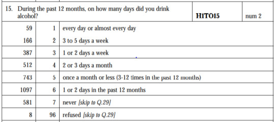
ANOVA revealed that among U.S. population who drink when they are not with family(H1TO13) and are White(H1GI6A) OR American Indian or Native American(H1GI6B) in race(subset1), frequency of drinks on days(collapsed into 6 ordered categories, which is the categorical explanatory variable) and quantity of drinks had each time per day (quantitative response variable) were relatively associated, F(5,1777)=27.63, p=5.09e-27<0.05 (p value is written in scientific notation). Post hoc comparisons of mean number of drinks each time by pairs of drinks frequency categories, revealed that those individuals drinking every day (or 3 to 5 days a week) reported drinking significantly more on average daily (every day: Mean=10.27, s.d.  ±9.47, 3 to 5 days a week: Mean=8.26, s.d.  ±5.57)  compared to those drinking 2 or 3 days a month (Mean=7.29, s.d.  ±8.16), or less. As a result, there are some pair cases in which frequency and drinking quantity of drinkers, are positive correlated.

In order to conduct post hoc paired comparisons in the context of my ANOVA, examining the association between frequency of drinks and number of drinks had each time, I used the Tukey HSD test. The table presented above, illustrates the differences in drinking quantity for each frequency of drinks use frequency group and help us identify the comparisons in which we can reject the null hypothesis and accept the alternate hypothesis, that is, in which reject equals true. In cases where reject equals false, rejecting the null hypothesis resulting in inflating a type 1 error.

[codezclub]

C Program to implement DFS Algorithm for Connected Graph

DFS Algorithm for Connected Graph Write a C Program to implement DFS Algorithm for Connected Graph. Here’s simple Program for traversing a directed graph through Depth First Search(DFS),  visiting only those vertices that are reachable from start vertex. Depth First Search (DFS) Depth First Search (DFS) algorithm traverses a graph in a depthward motion and uses a stack to remember to get the next…

[rollibar]

Process monitor linux

PROCESS MONITOR LINUX FREE

PROCESS MONITOR LINUX FREE

But feel free to combine both switches to get the exact behavior you want. With no -s option, the count option issues new output every second. For example, this command would run free 3 times, before exiting the program: If you only want free to run a certain number of times, you can use the -c (count option). To stop free from running, just press Ctrl+C. For example, to run the free command every 3 seconds: The -s (seconds) switch allows free to run continuously, issuing new output every specified number of seconds. This is handy if you want to see how memory is impacted while performing certain tasks on your system, such as opening a resource intensive program. But free also has some options for running continuously, in case you need to keep an eye on the usage for a while. When running the free command, it shows the current RAM utilization at that moment in time. This is the column you should look to if you simply want to answer “how much free RAM does my system have available?” Likewise, to figure out how much RAM is currently in use (not considering buffer and cache), subtract the available amount from the total amount. The number in this column is a sum of the free column and cached RAM that is available for reallocation. Total used free shared buffers cache availableĪvailable: This column contains an estimation (an accurate one, but nonetheless an estimation) of memory that is available for use. You can see these two columns separately by specifying the -w (wide) option: Most of the memory represented here can be reclaimed by processes whenever needed. Linux utilizes the buffer and cache to make read and write operations faster – it’s much quicker to read data from memory than from a hard disk. In Linux, tmpfs is represented as a mounted file system, though none of these files are actually written to disk – they are stored in RAM, hence the need for this column.įor the curious, a system’s tmpfs storage spaces can be observed with the df command:įilesystem Size Used Avail Use% Mounted onīuffer/Cache: This column contains the sum of the buffer and cache. As the name implies, this file system stores temporary files to speed up operations on your computer. Shared: This column displays the amount of memory dedicated to tmpfs, “temporary file storage”. As you can see in our example output above, our test machine has a measly 145 MB of memory that is totally free. There should ordinarily be a pretty small number here, since Linux uses most of the free RAM for buffers and caches, rather than letting it sit completely idle. The number in this column is the sum of total-free-buffers-cache.įree: This column lists the amount of memory that is completely unutilized. This makes read and write operations more efficient, but the kernel will reallocate that memory if a process needs it. While the “used” column does represent RAM which is currently in use by the various programs on a system, it also adds in the RAM which the kernel is using for buffering and caching. Just because memory is “in use” doesn’t necessarily mean that any process or application is actively utilizing it. Used: This column lists the amount of memory that is currently in use – but wait, that’s not quite as intuitive as it sounds. Total: This column is obvious – it shows how much RAM is physically installed in your system, as well as the size of the swap file. Let’s break down the details represented in all of these columns, since the terminology here gets a little confusing. This output tells us that our system has about 2 GB of physical memory, and about 1 GB of swap memory. Now the values are much clearer, even with a brief glance. The -h switch, which stands for “human readable”, helps us make more sense of the output: That’s chiefly because the output is given in kibibytes by default. Total used free shared buff/cache available

[uspscourse]

Data Analyst - Gapminder 2v3

1) Program: Gapminder2v3.py

import pandas import numpy import scipy import statsmodels.formula.api as sf_api import seaborn import matplotlib.pyplot as plt

""" any additional libraries would be imported here """

""" Set PANDAS to show all columns in DataFrame """ pandas.set_option('display.max_columns', None)

"""Set PANDAS to show all rows in DataFrame """ pandas.set_option('display.max_rows', None)

""" bug fix for display formats to avoid run time errors """ pandas.set_option('display.float_format', lambda x:'%f'%x)

""" read in csv file """ data = pandas.read_csv('gapminder.csv', low_memory=False) data = data.replace(r'^\s*$', numpy.NaN, regex=True)

""" checking the format of your variables """ data['country'].dtype

""" setting variables you will be working with to numeric """ data['employrate'] = pandas.to_numeric(data['employrate'], errors='coerce') data['internetuserate'] = pandas.to_numeric(data['internetuserate'], errors='coerce') data['lifeexpectancy'] = pandas.to_numeric(data['lifeexpectancy'], errors='coerce')

""" replace NaN to 0 and recoding to interger """ data['employrate'].fillna(0, inplace=True) data['internetuserate'].fillna(0, inplace=True) data['lifeexpectancy'].fillna(0, inplace=True) data['employrate']=data['employrate'].astype(int) data['internetuserate']=data['internetuserate'].astype(int) data['lifeexpectancy']=data['lifeexpectancy'].astype(int)

""" group data """ employ_gp=data.groupby('employrate').size() print("group employ rate among countries") print(employ_gp) net_gp=data.groupby('internetuserate').size()   print("group internet use rate among countries") print(net_gp) life_gp=data.groupby('lifeexpectancy').size() print("group life expectancy among countries") print(life_gp)

""" use ols function for F-statistic and associated p-value """ model_a = sf_api.ols(formula='employrate ~ C(internetuserate)', data=data).fit() print(model_a.summary())

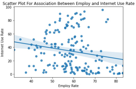
""" Scatter Plot For Association Between Employ and Internet Use Rate """ seaborn.regplot(x='employrate', y='internetuserate', fit_reg=True, data=data) plt.xlabel('Employ Rate') plt.ylabel('Internet Use Rate') plt.title('Scatter Plot For Association Between Employ and Internet Use Rate') plt.show()

""" Scatter Plot For Association Between Life Expectancy and Internet Use Rate """ seaborn.regplot(x='lifeexpectancy', y='internetuserate', fit_reg=True, data=data) plt.xlabel('Life Expectancy') plt.ylabel('Internet Use Rate') plt.title('Scatter Plot For Association Between Life Expectancy and Internet Use Rate') plt.show()

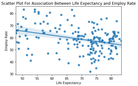
""" Scatter Plot For Association Between Life Expectancy and Employ Rate """ seaborn.regplot(x='lifeexpectancy', y='employrate', fit_reg=True, data=data) plt.xlabel('Life Expectancy') plt.ylabel('Employ Rate') plt.title('Scatter Plot For Association Between Life Expectancy and Employ Rate') plt.show()

""" fnd association between two variables """ data_clean=data.dropna()

print('Association between employ and internet use rate') print(scipy.stats.pearsonr(data_clean['employrate'], data_clean['internetuserate']))

print('Association between employ rate and life expectancy') print(scipy.stats.pearsonr(data_clean['employrate'], data_clean['lifeexpectancy']))

print('Association between employ internet use rate and life expectancy') print(scipy.stats.pearsonr(data_clean['internetuserate'], data_clean['lifeexpectancy']))

2) Output: Correlation coefficient

                           OLS Regression Results                             ============================================================================== Dep. Variable:             employrate   R-squared:                       0.387 Model:                            OLS   Adj. R-squared:                  0.045 Method:                 Least Squares   F-statistic:                     1.130 Date:                Sat, 27 Feb 2021   Prob (F-statistic):              0.266 Time:                        09:29:21   Log-Likelihood:                -923.45 No. Observations:                 213   AIC:                             2001. Df Residuals:                     136   BIC:                             2260. Df Model:                          76                                        

============================================================================== Omnibus:                        5.199   Durbin-Watson:                   2.181 Prob(Omnibus):                  0.074   Jarque-Bera (JB):                4.821 Skew:                          -0.332   Prob(JB):                       0.0898 Kurtosis:                       3.318   Cond. No.                         27.7 ==============================================================================

Notes: [1] Standard Errors assume that the covariance matrix of the errors is correctly specified. Association between employ and internet use rate (0.19505368645603788, 0.14969632618745277) Association between employ rate and life expectancy (0.2131830607630371, 0.11467385943527217) Association between employ internet use rate and life expectancy (0.7732949167937048, 2.8500749301451226e-12)

3) Testing the variables employrate, internetuserate and life expectancy for corretlation coefficient of all countries via scatter plots and stats (see output on item two for more details).

[marscratersdoug]

Second Mars Craters Post

First I found a couple of updates to the data set. http://craters.sjrdesign.net/#top This one seems to be the most recent, but it is lacking metadata on the fields. https://astrogeology.usgs.gov/search/map/Mars/Research/Craters/RobbinsCraterDatabase_20120821 is a couple of years older than the previous link, but it does have a link to metadata.

My first program follows:

import pandas # import numpy # import math # function to return number with thousand separator def formattedNumber(n):  return ("{:,}".format(n)) # CRATER_ID,LATITUDE_CIRCLE_IMAGE,LONGITUDE_CIRCLE_IMAGE df = pandas.read_csv('Mars Craters IIb.csv', low_memory=False) TotalCraters = len(df) # print (TotalCraters) #number of observations (rows) # print (len(df.columns)) # number of variables (columns) df['LATITUDE_CIRCLE_IMAGE']  = pandas.to_numeric(df['LATITUDE_CIRCLE_IMAGE']) df['LONGITUDE_CIRCLE_IMAGE'] = pandas.to_numeric(df['LONGITUDE_CIRCLE_IMAGE']) NorthernHemisphere=df[(df['LATITUDE_CIRCLE_IMAGE']>=0)] NH = NorthernHemisphere.copy() SouthernHemisphere=df[(df['LATITUDE_CIRCLE_IMAGE']<0)] SH = SouthernHemisphere.copy() EasternHemisphere=df[(df['LONGITUDE_CIRCLE_IMAGE']>=0)] EH = EasternHemisphere.copy() WesternHemisphere=df[(df['LONGITUDE_CIRCLE_IMAGE']<0)] WH = WesternHemisphere.copy() print("Total Craters: %s" % (formattedNumber(TotalCraters))) print("Number of craters in the %s:%s Percent of total:%s%%\n" % ('Northern Hemisphere', formattedNumber(len(NH)), formattedNumber((len(NH) / TotalCraters) * 100))) print("Number of craters in the %s:%s Percent of total:%s%%\n" % ('Southern Hemisphere', formattedNumber(len(SH)), formattedNumber((len(SH) / TotalCraters) * 100))) print("Number of craters in the %s:%s Percent of total:%s%%\n" % ('Eastern Hemisphere',  formattedNumber(len(EH)), formattedNumber((len(EH) / TotalCraters) * 100))) print("Number of craters in the %s:%s Percent of total:%s%%\n" % ('Western Hemisphere',  formattedNumber(len(WH)), formattedNumber((len(WH) / TotalCraters) * 100))) QuadrantB=df[(df['LATITUDE_CIRCLE_IMAGE']>=0) & (df['LONGITUDE_CIRCLE_IMAGE']>=0)] QB = QuadrantB.copy() QuadrantD=df[(df['LATITUDE_CIRCLE_IMAGE']>=0) & (df['LONGITUDE_CIRCLE_IMAGE']<0)] QD = QuadrantD.copy() QuadrantA=df[(df['LATITUDE_CIRCLE_IMAGE']<0) & (df['LONGITUDE_CIRCLE_IMAGE']>=0)] QA = QuadrantA.copy() QuadrantC=df[(df['LATITUDE_CIRCLE_IMAGE']<0) & (df['LONGITUDE_CIRCLE_IMAGE']<0)] QC = QuadrantC.copy() print("Total Craters: %s" % (formattedNumber(TotalCraters))) print("Number of craters in the %s:%s Percent of total:%s%%\n" % ('Quadrant A', formattedNumber(len(QA)), formattedNumber((len(QA) / TotalCraters) * 100))) print("Number of craters in the %s:%s Percent of total:%s%%\n" % ('Quadrant B', formattedNumber(len(QB)), formattedNumber((len(QB) / TotalCraters) * 100))) print("Number of craters in the %s:%s Percent of total:%s%%\n" % ('Quadrant C', formattedNumber(len(QC)), formattedNumber((len(QC) / TotalCraters) * 100))) print("Number of craters in the %s:%s Percent of total:%s%%\n" % ('Quadrant D', formattedNumber(len(QD)), formattedNumber((len(QD) / TotalCraters) * 100)))

This program calculates hemisphere and quadrant information for each crater. The percentages for each. The output is below:

runfile('C:/src/py/MarsCraters/Mars Craters Geographic Distribution.py', wdir='C:/src/py/MarsCraters') Total Craters: 384,278 Number of craters in the Northern Hemisphere:150,913 Percent of total:39.27182924861688% Number of craters in the Southern Hemisphere:233,365 Percent of total:60.72817075138312% Number of craters in the Eastern Hemisphere:210,341 Percent of total:54.73667501131993% Number of craters in the Western Hemisphere:173,937 Percent of total:45.26332498868007% Total Craters: 384,278 Number of craters in the Quadrant A:150,913 Percent of total:39.27182924861688% Number of craters in the Quadrant B:150,913 Percent of total:39.27182924861688% Number of craters in the Quadrant C:150,913 Percent of total:39.27182924861688% Number of craters in the Quadrant D:150,913 Percent of total:39.27182924861688% runfile('C:/src/py/MarsCraters/Mars Craters Geographic Distribution.py', wdir='C:/src/py/MarsCraters') Total Craters: 384,278 Number of craters in the Northern Hemisphere:150,913 Percent of total:39.27182924861688% Number of craters in the Southern Hemisphere:233,365 Percent of total:60.72817075138312% Number of craters in the Eastern Hemisphere:210,341 Percent of total:54.73667501131993% Number of craters in the Western Hemisphere:173,937 Percent of total:45.26332498868007% Total Craters: 384,278 Number of craters in the Quadrant A:122,071 Percent of total:31.766325420659% Number of craters in the Quadrant B:88,270 Percent of total:22.970349590660927% Number of craters in the Quadrant C:111,294 Percent of total:28.961845330724113% Number of craters in the Quadrant D:62,643 Percent of total:16.30147965795596%

I created a subset of the whole dataset with just CRATER_ID, LATITUDE_CIRCLE_IMAGE, and LONGITUDE_CIRCLE_IMAGE. These are the only fields required to calculate the geographic values I am looking at.

I am also working on a python script to calculate distances between the craters in order to look for clusters of craters.

[strangehoot]

New Post has been published on Strange Hoot - How To’s, Reviews, Comparisons, Top 10s, & Tech Guide

New Post has been published on https://strangehoot.com/how-to-install-hive-on-windows-10/

How to Install Hive on Windows 10

“Install Hive on Windows 10” is not an easy process. You need to be aware of prerequisites and a basic understanding of how the Hive tool works. Big Data Hadoop is known to people who are into data science and work in the data warehouse vertical. Large data can be handled via Big Data Hadoop framework. 

In this article, we are going to see how you install Hive (a data query processing tool) and have it configured in the Hadoop framework.

Prerequisites to successfully perform Hive Installation

Before you start the process of installing and configuring Hive, it is necessary to have the following tools available in your local environment. 

If not, you will need to have the below software for Hive to be working appropriately.

Java 

Hadoop

Yarn 

Apache Derby

Install Hive on Windows 10 [step-by-step guide]

Check whether Java is available in your machine. Follow the steps below to verify the same.

Initiate CMD window.

Enter the text as a command below and hit ENTER.

C:\Users\Administrator\java -version

You will see the details as output shown below.

In case your Java version is older, you will need to update by following the next steps.

In the search bar at the bottom left, enter the keyword “About java”.

You will see the search results available. 

Open the Java app. The pop up appears as below.

Click the link shown in the text, you will be redirected to the Java webpage.

Click the red (agree and start free download) button shown in the image below.

An exe file will be downloaded and saved in your Downloads folder.

Run the exe file by double-clicking. See below.

You will get a prompt that states the old version is available in the system.

Choose Uninstall. 

Choose the Next option. Once the new version is installed, you will see the success message as below.

Choose Close to shut the window.

Install Hadoop 3.3.0 in your Windows 10.

Download the package from https://hadoop.apache.org/release/3.3.0.html 

Click the top right corner green button that says “Download tar.gz”.

Once downloaded, check whether Java is installed. 

NOTE: We already have installed / updated Java in the previous step. Java JDK 8 is the prerequisite for Hadoop installation.

Before we proceed with installation steps, make sure your Java is installed in your root drive (c:\). If not, please move the folder from C:\Program Files to C:\Java. 

NOTE: This will avoid conflict while setting environment variables.

In your Windows 10 System Settings, search for environment settings.

Choose the option Edit system environment variables.

Click the button that says Environment Variables. See the image below.

Add a new variable by clicking New. 

Enter the name as JAVA-HOME. 

Enter the path where Java is located. Java path for us is under C:\Java\jdknamwithversion\bin.

Once the new variable is set, edit the path variable.

To do so, select the Path variable and click Edit.

Click New and paste the path.

Check Java is working as expected by entering the command javac from the command line window.

Now, go to the folder where hadoop tar.gz is downloaded.

Extract hadoop-3.3.0.tar.gz. You will get another tar file.

Extract hadoop-3.3.0.tar. Once done, you will see the extracted folder.

Copy the folder hadoop-3.3.0 in your C:\ drive.

Edit 5 files under this folder. Go to C:\hadoop-3.3.0\etc\hadoop.

core-site.xml

hadoop-env.cmd

hdfs-site.xml

mapred-site.xml

yarn-site.xml

Open these files in notepad editor.

Enter the code below in the core-site.xml file.

<configuration> <property> <name>fs.default.name</name> <value>hdfs://localhost:9000</value> </property></configuration>

Enter the code below in the mapred-site.xml file.

<configuration> <property> <name>mapreduce.framework.name</name> <value>yarn</value> </property></configuration>

Enter the code below in the yarn-site.xml file.

<configuration> <property> <name>yarn.nodemanager.aux-services</name> <value>mapreduce_shuffle</value> </property> <property> <name>yarn.nodemanager.auxservices.mapreduce.shuffle.class</name><value>org.apache.hadoop.mapred.ShuffleHandler</value> </property></configuration>

Create 2 folders “datanode” and “namenode” in your C:\hadoop-3.3.0\data folder before we update the hdfs-site.xml. The folder paths will look like this.

C:\Hadoop-3.3.0\data\datanodeC:\Hadoop-3.3.0\data\namenode

Enter the code below in the hdfs-site.xml.

<configuration> <property><name>dfs.replication</name> <value>1</value> </property> <property> <name>dfs.namenode.name.dir</name> <value>file:///C:/hadoop-3.3.0/data/namenode</value> </property> <property> <name>dfs.datanode.data.dir</name> <value>/C:/hadoop-3.3.0/data/datanode</value> </property></configuration>

Set the JDK path into the hadoop-env.cmd file as below.

Save all the files we updated as above.

Next, set the HADOOP path variable from Windows 10 system settings.

Choose the option Edit system environment variables.

Click the button that says Environment Variables. 

Create a new variable HADOOP_HOME.

Set the path as C:\hadoop-3.3.0\bin.

Edit the path variable and set the path of Hadoop as below.

Enter C:\hadoop-3.3.0\bin and OK.

Set another path for the sbin folder. Perform the same step as above.

Now, go to the bin folder under your hadoop-3.3.0 folder.

Copy configuration files for Hadoop under this folder. Please refer to the Configuration zip file to copy the files.

Delete the existing bin folder and copy the bin folder from this configuration.zip to C:\hadoop-3.3.0\.

You are ready as you have successfully installed hadoop. To verify success, open CMD as administrator, enter the command below.

You will get the message as below.

Now, the next step is to start all the services. If your installation is successful, go to your sbin directory and enter the command as below.

You will see namenode and datanode windows will start after executing the above command.

Then, give the command, start-yarn. Two yarn windows will open up and will keep running.

NOTE: If all of the above resource files do not shut down automatically, be assured that your installation and configuration is successful.

Enter the command jps. You will see a number of processes running on all four resources.

To access Hadoop, open your browser and enter localhost:9870. You will see below.

To check yarn, enter localhost:8088 in a new window.

Now, you are ready to install Hive. Download the package from https://downloads.apache.org/hive/hive-3.1.2/ by clicking the apache-hive-3.1.2-bin.tar.gz link.

Extract the folder using the 7zip extractor. Once extracted, you will see hive-3.1.2.tar file. Extract the same again.

The way we have set environment variables for hadoop, we need to set the environment variable and path for Hive too.

Create the following variables and their paths.

HIVE_HOME: C:\hadoop-3.3.0\apache-hive-3.1.2\

DERBY_HOME: C:\hadoop-3.3.0\db-derby-10.14.2.0\

HIVE_LIB: %HIVE_HOME%\lib

HIVE_BIN: %HIVE_HOME%\bin  

HADOOP_USER_CLASSPATH_FIRST: true

Set the above path for each variable as shown after “:”.

Copy and paste all Derby libraries (.jar files) from derby package to the Hive directory: C:\hadoop-3.3.0\apache-hive-3.1.2\lib

Locate hive-site.xml in the bin directory. Enter the code below in the XML file.

Start hadoop services by: start -dfs and start-yarn as we saw in the Hadoop section above.

Start derby services by: C:\hadoop-3.3.0\db-derby-10.14.2.0\bin\StartNetworkServer -h 0.0.0.0

Start hive service by: go to your Hive bin directory through the command line. Enter hive. If that command doesn’t work, the following message will be shown.

NOTE: This is due to Hive 3.x.x version not supporting the commands in Windows 10. You can download the cmd libraries from the https://github.com/HadiFadl/Hive-cmd link. Also, replace the guava-19.0.jar to guava-27.0-jre.jar from the Hadoop’s hdfs\lib folder.

Once done, run the command hive again. It should be executed successfully.

Metastore initialization after starting the hive service.

NOTE: Again, you will need to use the cgywin tool to execute linux commands in Windows.

Create the 2 folders: C:\cygdrive and E:\cygdrive.

Open the command window and enter the following commands.

Specify the environment variables as below.

Enter the command below to initialize Metastore.

Now, open the command window and enter the command as shown below.

Open another command window and type hive. You should be able to successfully start hive service.

Install Hive on Windows 10 is a complicated process

As we saw, version 3.x.x of Hive is a little difficult to install in the Windows machine due to unavailability of commands support. You will need to install a commands library that supports linux based commands to initialize Metastore and Hive services for successful execution.

If you set environment variables and path correctly in Hadoop and Hive configuration, life will become easier without getting errors on starting the services. 

In this article, you have got an overview on the steps on “install hive on Windows 10”.

Read More: How to Install Server Nginx on Ubuntu

[codeavailfan]

Assembly Language Homework Help

Assembly Language Assignment Support . Assembly Language Homework Support

If you think assembly language is a difficult programming subject, you are not the only student who makes the subject challenging. Out of every 100 programming assignments to be submitted on our website, 40 are in the conference language. Assembly language assignment is the most sought service in support programming. We have a team of expert programmers who work only on assembly language projects. They go first through the directions of the university for the students and then start the project. They not only share the complete programming work that can be easily run but they are successfully running the screen shot of the program and share a step-by-step approach to how students can understand and implement the program.

If you are one of those students who do not have the full knowledge of concepts, it is difficult for you to complete the assembly language homework. The Programming Assignment Support website can provide you with the Executive Assembly Language homework help Solution. Before we go ahead, let's learn more about the assembly language.

What is assembly language?

Assembly language is a low-level programming language which is a correspondence between machine code and program statement. It is still widely used in academic work. Assembly is the main application of language - it is used for equipment and micro-controllers. It is a collection of languages which will be used to write machine codes for creating CPU architecture. However, there will be no required functions and variables in this language and cannot be used in all types of processors. Assembly language commands and structures are similar to machine language, but it allows the programmer to use the number with the names.

A low-level language is a language that works with computer hardware. Gradually, they forgot. These languages are still kept in the curriculum as it gives students hardware knowledge

Here are some important concepts in assembly language:

Collecter

Language Design - Opcode Memonics and Detailed Nemonics, Support for ureded programs, Assembly Instructions and Data Instructions

Operators, Parts and Labels

Machine Language Instructions

Maths and Transfer Instructions

Pageing, catch and interruptions

These are just a few topics; We will work on many other subjects in accordance with the needs of the students to assist in assembly language assignment.

Key concepts to be learned in assembly language

The following 6 important vocabularies in Assembly Languedhoes are given below

Memory address: This is where the machine will store code. If the address starts with YY00, YY represents the page number and the 00 line number.

Machine Code: It is also called the instruction code. This code will include hexadecimal numbers with instructions to store memory address.

Label: A collection of symbols to represent a particular address in a statement. The label has colons and is found whenever necessary.

Operation Code: This instruction contains two main parts. Operand and Opcodes. The opcode will indicate the function type or function to be performed by the machine code.

Operade: This program contains 8-bit and 16-bit data, port address, and memory address and register where the instructions are applied. In fact, the instruction is called by another name, namely namonic which is a mixture of both opcode and opred. Notenotes english characters which are initial to complete the work by directing. The memoric used to copy data from one place to another is mov and sub for reduction.

Comments: Although, they are not part of programming, they are actually part of the documents that describe actions taken by a group or by each directive. Comments and instructions are separated by a colon.

What is included in an assembly language assignment program?

Assembly Language homework help includes the concepts below which are used to reach a solution.

Mu Syle Syntax - Assembly Language Program can be divided into 3 types - Data Section, BSS section, Text Section

Statements - There are three types of assembly language statements - Directors, Macros and Executive Instructions These statements enter 1 statement in each line

The assembly language file is then saved as a .asm file and run the program to get the required output

What are assembly registers?

Processor operation mostly works on processing data. Registers are internal memory storage spaces that help speed up the processor's work. In IA-32, there are six 16-bit processor registers and ten 32-bit registers. Registers can be divided into three categories -

General Register

Data Register - 32-bit Data Register: EAX, EBX, ECX, EDX. X is primary collector, BX is base register, C x counter is registered and DX is data register.

Pointer Register - These are 32-bit EIP, ESP, and EBP registers. There are three types of pointers like Instruct Pointer (IP), Stack Pointer (SP) and Base Pointer (BP)

Index Register - These registers are divided into Resource Index (SI) and Destination Index (DI)

Control Register - Control Registers can be defined as a combination of 32-bit Directive Director Register and 32-bit Flags Register. Some of the bits of the famous flag are overflow flag (off), trap flag (TF), enterprise flag (IF), sign flag (SF), Disha Flag (DF), Zero Flag (ZF).

Sugar Register - These are further divided into code segments, data segments and stack sections

Assembly Language Functions

The main benefit given by assembly language is the speed on which the programmes are run. Anyone in the assembly language can write instructions five times faster than the Pascal language. Moreover, the instructions are simple and easy to interpret code and work for microprocessors. With assembly language, it is easy to modify the instructions of a program. The best part is that the symbols used in this language are easy to understand, thus leaving a lot of time left for the programs. This language will enable you to develop an interface between different pieces of code with the help of inconsistent conferences.

The lack of benefits mentioned above are different applications of assembly language. Some of the most common tasks are given below:

Assembly language is used to craft code to boot the system. Code operating system will be helpful in booting and starting system hardware before storing it in ROM

Assembly language is complete to promote working speed despite low processing power and RAM

Here are some compilers that allow you to translate the high level language into assembly language before you complete the compilation. This will allow you to see the code for the debugging and optimization process.

As you read the page, you can easily conclude that the assembly language will require complex coding. Not all students have the right knowledge of programming and therefore use the 'Programming Assignment Assistance' to complete their programme language lecture on time. If you have difficulty completing the assignment and want to get rid of the stressful process of completing the assignment on your own, the advantage of our Assembly Language Programming Services is to ensure that you get a + grade in all projects.

Assembly Language Assignment Support . Assembly Language Homework Support

We are receiving our Bachelor's and Masters degrees by offering programming homework support to the students of programming and computer science in various universities and colleges around the world.

Our Assembly Language Assignment Support Service is a fit for your budget. You only have to pay a pocket-friendly price to get the running assembly language project no matter how difficult it may be.

Assignment can deal with any of the following subject: Intel Processor, 6502 - 8 bit processor, 80 × 86 - 16 bit processor, 68000 - 32 bit processor, dos emulator, de-morgan theory, assembly basic syntax, assembly memory. Sections etc. Our experts ensure that they provide quality work for Assembly Language Assignment Support as they are aware of the complete syllabus and can use concepts to provide assignments in accordance with your academic needs.

Instructions are used to complete assembly language assignment. Some common instructions include EKU, ORG, DS, =, ID, ENT, IF, IFNOT, ELSE, EDF, RESET, EOG and EEDTA. These instructions instruct the collecter to work. The use of correct instructions is very important in completing the successful project. Our experts ensure that they meet global standards while completing assembly language homework. If you take the support of our programmers to the assembly language homework, you don't have to worry about the quality of the solution.

Why should you set assembly language?

Assembly language is best for writing ambedded programs

This improves your understanding of the relationship between computer hardware, programs and operating systems.

The speed required to play the computer game. If you know assembly language, you can customize the code to improve the program speed

Low-level tasks such as data encryption or bitwise manipulation can be easily done using assembly language

Real-time applications that require the right time and data can be easily run using assembly language.

Why choose the 'Programming Assignment Help' service?

Our service is USP - we understand that you are a student and getting high ratings at affordable prices is what we have to offer programming assistance that we provide on all subjects. Our assembly language-specific support is unique in many ways. Some of them are given below:

Nerdi Assembly Language Expert: We have 346 programmers who work on assembly language projects only. They must have been solved near 28,512 work and domestic work so far

100% Original Code: We provide unique solutions otherwise you get a full refund. We dismiss the expert if he shares the 1 theft solution.

Pocket Friendly: Support for assembly language homework help is expensive because it is one of the most important topics in programming. We ensure that we provide affordable rates to our students. Repeating customers can get 10% off from the third order.

Free Review: We share screenshots of the program normally running so that there is no need for modification. However, if you still need to modify the work, we provide free price modifications within 5-6 hours.

85% Repeat Customer: We will do things right for the first time. Our programmers have complete code writing experience. Keeping good programmers has resulted in 85% repetition and 98% customer satisfaction.

If you are still looking for support for assembly language tasks and home works, please send us an email or talk to our customer care executive and we will lead you to complete the work and get a grade.

[wemakenoclaims]

Data Analysis Tools - Week 1 - Running An Analysis of Variance

INTRODUCTION / OVERVIEW

We return to my research question from the beginning of this 4 course / 1 capstone program. By the end of my last entry (Data Management and Visualization - Week 4 - Visualizing Data), I kept recognizing that I wanted to interpret my data in ways that were beyond what we’d been taught...and it looks like that was just a nice segue for what we’d learn in this course. (Almost like they put the courses in a certain order for a reason.)

For reference, my original research question and hypothesis.

/// /// /// /// /// /// /// /// /// /// /// /// /// /// /// ///

Research question - How and to what extent does a nation’s CO2 emissions correlate with the percentage of its labor force that is in the military?

Hypothesis - My hypothesis is the GapMinder dataset will demonstrate a high positive correlation between my chosen variables ”armedforcesrate” and ”co2emissions.” I’d like to note, this was my intuitive hypothesis before I began my literature review, and I tried to look out for potential issues of confirmation bias. Although I wasn’t able to find any research (in my admittedly surface review) that took a directly opposing view, it did seem that there is debate to how much militarism itself is an independent driver, as opposed to be being an outgrowth of developed economies.

/// /// /// /// /// /// /// /// /// /// /// /// /// /// /// ///

Although I will get to run an inference test against the comparison of these quantitative variables as quantitative variables (i.e. Q->Q) at some point, that requires a correlation coefficient test, like Pearson Correlation, which we will learn in week 3.

For now, using the Analysis of Variance (ANOVA) test learned this week, we can conduct a comparable inference test after converting my explanatory (x) quantitative variable into a categorical variable (i.e. C->Q). I’ll therefore do a bivariate comparison of the quartiles of ‘armedforcesrate’ to the means of ‘co2emissions.’

I ran that comparison last week, in the post which is linked in first paragraph above. For brevity, I am including the bar chart only; you can follow that link to see the work behind the results.

INFERENCE TEST - ANOVA / ORDINARY LEASED SQUARES

The Null Hypothesis (H0) - There is no relationship between a nation’s CO2 emissions and the percentage of its total labor force employed by the military.

The Alternate Hypothesis (Ha, or H1) - There is a relationship between a nation’s CO2 emissions and the percentage of its total labor force employed by the military. (Notably, Ha makes no statement about what that relationship is, only that some relationship exists).

The ANOVA F-test is used to determine whether we can reject the null hypothesis and accept the alternate hypothesis. F is calculated as shown below...

                       [variation among sample means]

  F =                ------------------------------------------

                        [variation within sample groups]

...and generally, if the variation among sample means "wins out” it will provide a larger F which corresponds to a lower p, or a lower probability that the variations between groups occured based on random chance alone. For our purposes, if p <= 0.05, i.e. 5% or lower, we consider the results statistically significant and we can reject the null hypothesis.

///CODE///

# -*- coding: utf-8 -*- # import packages needed for my program import pandas as pd import numpy as np import seaborn as sb import matplotlib.pyplot as plt import statsmodels.formula.api as smf import statsmodels.stats.multicomp as multi

#pandas statement to avoid run time error# pd.set_option('display.float_format',lambda x:'%f'%x)

#pandas statement to set max rows and columns for the long/wide lists associated with distro of two of my variables pd.options.display.max_rows = 300 pd.options.display.max_columns = 200

#pandas show ver, disabled unless I need it for troubleshooting ##pd.show_versions()

#read in the data from the GapMinder dataset, and convert the column names to lowercase data = pd.read_csv ('_5e80885b18b2ac5410ea4eb493b68fb4_gapminder.csv', low_memory = False) data.columns = map (str.lower, data.columns)

#ensure numerical values are not misinterpreted as strings due to blanks data['co2emissions']=pd.to_numeric(data['co2emissions'],errors="coerce") data['armedforcesrate']=pd.to_numeric(data['armedforcesrate'],errors="coerce")

#make a copy of my dataset. ##NOTE: I named it "sub2" for consistency with the lessons, but I didn't use a subset of my dataframe as the initial basis ##more commonly there'd be a 'sub1' defined as only the rows matching certain values, and then sub2 is the safety copy of it sub2 = data.copy()

#!!!!!!Course2Week1 material (ANOVA) starts here!!!!!

#Create new x/explanatory variable from armedforcesrate, split into quartiles sub2['armedforcesrate4'] = pd.qcut(sub2.armedforcesrate, 4, labels =['1=25%tile','2=50%tile','3=75%tile','4=100%tile'])

#ANOVA OLS here sub3=sub2[['co2emissions', 'armedforcesrate4']].dropna() model1=smf.ols(formula = 'co2emissions ~ C(armedforcesrate4)',data = sub3) results1=model1.fit() print('Analysis of Variance (ANOVA) - Ordinary Lease Squares (OLS) Regression to get F-statistic') print('') print(results1.summary()) print('')

///OUTPUT///

(first as image - click to enlarge)

(second as text - may be easier to see than the image, but formatting suffers)

Analysis of Variance (ANOVA) - Ordinary Lease Squares (OLS) Regression to get F-statistic

                           OLS Regression Results                             ============================================================================== Dep. Variable:           co2emissions   R-squared:                       0.009 Model:                            OLS   Adj. R-squared:                 -0.010 Method:                 Least Squares   F-statistic:                    0.4868 Date:                Fri, 28 Aug 2020   Prob (F-statistic):              0.692 Time:                        18:40:51   Log-Likelihood:                -4128.4 No. Observations:                 162   AIC:                             8265. Df Residuals:                     158   BIC:                             8277. Df Model:                           3                                         Covariance Type:            nonrobust                                         =====================================================================================================                                        coef    std err          t      P>|t|      [0.025      0.975] ----------------------------------------------------------------------------------------------------- Intercept                          5.053e+09   4.53e+09      1.116      0.266   -3.89e+09     1.4e+10 C(armedforcesrate4)[T.2=50%tile]   1.469e+09    6.4e+09      0.230      0.819   -1.12e+10    1.41e+10 C(armedforcesrate4)[T.3=75%tile]   5.205e+09   6.36e+09      0.818      0.415   -7.36e+09    1.78e+10 C(armedforcesrate4)[T.4=100%tile] -2.221e+09   6.36e+09     -0.349      0.727   -1.48e+10    1.03e+10 ============================================================================== Omnibus:                      308.309   Durbin-Watson:                   1.721 Prob(Omnibus):                  0.000   Jarque-Bera (JB):            76187.144 Skew:                           9.642   Prob(JB):                         0.00 Kurtosis:                     107.475   Cond. No.                         4.82 ==============================================================================

///ANALYSIS///

F = 0.4868,

This tells us that variation within sample groups, the denominator in our equation, was greater than the variation among sample means across the board. Recall that a comparatively large numerator would be expected if the variation among sample means was “winning out.”

p = 0.692

This is > .05 by a long shot, and thus we do not have sufficient evidence to reject the null hypothesis. This can be read as more than 69 times out of 100, we would be wrong to reject it.

The post hoc paired comparison test that follows therefore isn’t necessary...or even advised! It applies to situations where there are more than 2 categories in the explanatory variable (we have that), requiring additional comparisons to learn more about the relationship between the variables without introducing Family-wise errors (the rate of Family-wise errors is a given if we simply reran ANOVA for each pair), and p of the R-statistic was <= 0.5 giving us evidence to reject the null hypothesis (we don’t have that).

POST HOC PAIRED COMPARISONS

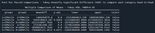
As noted, the ANOVA/OLS results already told us we had insufficient evidence to reject the null hypothesis, and this post hoc test is therefore only for demonstration purposes. The specific post hoc test is Tukey’s Honestly Significant Difference.

///CODE///

#Post hoc (Tukey HSD) here mc1=multi.MultiComparison(sub3['co2emissions'], sub3['armedforcesrate4']) results2=mc1.tukeyhsd() print('Post hoc Paired Comparisons - Tukey Honestly Significant Difference (HSD) to compare each category head-to-head') print('') print(results2.summary()) print('')

///OUTPUT///

(first as image - click to enlarge)

(second as text - may be easier to see than the image, but formatting suffers)

Post hoc Paired Comparisons - Tukey Honestly Significant Difference (HSD) to compare each category head-to-head

                Multiple Comparison of Means - Tukey HSD, FWER=0.05                   ======================================================================================  group1    group2       meandiff     p-adj        lower            upper       reject -------------------------------------------------------------------------------------- 1=25%tile  2=50%tile     1469284575.0    0.9  -15154094813.236  18092663963.236  False 1=25%tile  3=75%tile   5204746024.187 0.8264 -11316960365.0894 21726452413.4634  False 1=25%tile 4=100%tile -2221319097.7642    0.9 -18743025487.0406 14300387291.5122  False 2=50%tile  3=75%tile   3735461449.187    0.9 -12786244940.0894 20257167838.4634  False 2=50%tile 4=100%tile -3690603672.7642    0.9 -20212310062.0406 12831102716.5122  False 3=75%tile 4=100%tile -7426065121.9512 0.6271 -23845468940.0466  8993338696.1442  False

///ANALYSIS///

A positive meandifference tells us group1′s mean is lower than group2′s, and a negative meandifference tells us group2′s mean is lower than group1′s. That’s true of the sample, but it is only considered statistically significant (i.e. likely to be true of the population) where p is <= 0.05 for that specific paired comparisons in the post hoc test. And in our case, p > 0.05 in all paired comparisons. While p itself is not shown in the table, it’s driving the output in the last column, labeled “reject.”

IF any of the paired comparisons had p <= 0.05, this would display “True” and the null hypothesis could be rejected at the level of these two categories specifically.

In our case, all display “False,” and we should not consider any of the paired comparisons to be statistically significant. This makes intuitive sense given the ANOVA results already told us p was 0.692 and by process we would not even proceed to run this post hoc test, though admittedly I do not know if this intuition is correct i.e. would hold for all cases.

///CONCLUSIONS///

In summary:

The null hypothesis is that there is no association between the ‘armedforcesrate4′ categorical explanatory variable and the ‘co2emissions’ quantitative response variable.

Our data do not provide sufficient evidence to reject the null hypothesis, by virtue of the F-statistic obtained in the ANOVA Ordinary Lease Squares inference test having a p > 0.05 (it was 0.692 specifically). We would expect to be wrong to do so over 69 times out of 100.

Our data also do not provide sufficient evidence to result the null hypothesis at the level of any specific paired comparisons, by virtue of each paired comparison showing reject = “False” in the post hoc Tukey’s Honestly Significant Difference test. We also wouldn’t have turned to this test in a “real world” situation, given the outcome of the OLS inference test above.

[deepppp13]

Hypothesis Testing and Chi Square Test of Independence

This assignment aims to directly test my hypothesis by evaluating, based on a sample of 4946 U.S. which resides in South region(REGION) aged between 25 to 40 years old(subsetc1), my research question with a goal of generalizing the results to the larger population of NESARC survey, from where the sample has been drawn. Therefore, I statistically assessed the evidence, provided by NESARC codebook, in favor of or against the association between Cigars smoked status and fear/avoidance of heights, in U.S. population in the South region. As a result, in the first place I used crosstab function, in order to produce a contingency table of observed counts and percentages for fear/avoidance of heights. Next, I wanted to examine if the Cigars smoked status (1= Yes or 2=no) variable ‘S3AQ42′, which is a 2-level categorical explanatory variable, is correlated with fear/avoidance of heights (’S8Q1A2′), which is a categorical response variable. Thus , I ran Chi-square Test of Independence(C->C) and calculated the  χ-squared values and the associated p-values for our specific conditions, so that null and alternate hypothesis are specified. In addition, in order visualize the association between frequency of cannabis use and depression diagnosis, I used catplot function to produce a bivariate graph. Furthermore, I used crosstab function once again and tested the association between the frequency of cannabis use (’S3BD5Q2E’), which is a 10-level categorical explanatory variable. In this case, for my second Test of Independence (C->C), after measuring the χ-square value and the p-value, in order to determine which frequency groups are different from the others, I performed a post hoc test, using Bonferroni Adjustment approach, since my explanatory variable has more than 2 levels. In this case of ten groups, I actually need to conduct 45 pair wise comparisons, but in fact I examined indicatively two and compared their p-values with the Bonferroni adjusted p-value, which is calculated by dividing p = 0.05 by 45. By this way it is possible to identify the situations where null hypothesis can be safely rejected without making an excessive type 1 error. For the code and the output I used Jupyter Notebook(IDE).

PROGRAM:

import pandas as pd

import numpy as np

import scipy.stats

import seaborn

import matplotlib.pyplot as plt

data = pd.read_csv('nesarc_pds.csv',low_memory=False)

data['AGE'] = pd.to_numeric(data['AGE'],errors='coerce')

data['REGION'] = pd.to_numeric(data['REGION'],errors='coerce')

data['S3AQ42'] = pd.to_numeric(data['S3AQ42'],errors='coerce')

data['S3BQ1A5'] = pd.to_numeric(data['S3BQ1A5'],errors='coerce')

data['S8Q1A2'] = pd.to_numeric(data['S8Q1A2'],errors='coerce')

data['S3BD5Q2E'] = pd.to_numeric(data['S3BD5Q2E'],errors='coerce')

data['MAJORDEP12'] = pd.to_numeric(data['MAJORDEP12'],errors='coerce')

subset1 = data[(data['AGE']>=25) & (data['AGE']<=40) & (data['REGION']==3)]

subsetc1 = subset1.copy()

subset2 = data[(data['AGE']>=18) & (data['AGE']<=30) & (data['S3BQ1A5']==1)]

subsetc2 = subset2.copy()

subsetc1['S3AQ42'] = subsetc1['S3AQ42'].replace(9,np.NaN)

subsetc1['S8Q1A2'] = subsetc1['S8Q1A2'].replace(9,np.NaN)

subsetc2['S3BD5Q2E'] = subsetc2['S3BD5Q2E'].replace(99,np.NaN)

cont1 = pd.crosstab(subsetc1['S8Q1A2'],subsetc1['S3AQ42'])

print(cont1)

colsum = cont1.sum()

contp = cont1/colsum

print(contp)

print ('Chi-square value, p value, expected counts, for fear/avoidance of heights within Cigar smoked status')

chsq1 = scipy.stats.chi2_contingency(cont1)

print(chsq1)

cont2 = pd.crosstab(subsetc2['MAJORDEP12'],subsetc2['S3BD5Q2E'])

print(cont2)

colsum = cont2.sum()

contp2 = cont2/colsum

print(contp2)

print('Chi-square value, p value, expected counts, for major depression within cannabis use status')

chsq2 = scipy.stats.chi2_contingency(cont2)

print(chsq2)

recode = {1:10,2:9,3:8,4:7,5:6,6:5,7:4,8:3,9:2,10:1}

subsetc2['CUFREQ'] = subsetc2['S3BD5Q2E'].map(recode)

subsetc2['CUFREQ'] = subsetc2['CUFREQ'].astype('category')

subsetc2['CUFREQ'] = subsetc2['CUFREQ'].cat.rename_categories(['Once a year','2 times a year','3 to 6 times a year','7 to 11 times a year','Once a month','2 to 3 times a month','1 to 2 times a week','3 to 4 times a week','Nearly Everyday','Everyday'])

plt.figure(figsize=(16,8))

ax1 = seaborn.catplot(x='CUFREQ',y='MAJORDEP12', data=subsetc2, kind="bar", ci=None)

ax1.set_xticklabels(rotation=40, ha="right")

plt.xlabel('Frequency of cannabis use')

plt.ylabel('Proportion of Major Depression')

plt.show()

recode={1:1,9:9}

subsetc2['COMP1v9'] = subsetc2['S3BD5Q2E'].map(recode)

cont3 = pd.crosstab(subsetc2['MAJORDEP12'],subsetc2['COMP1v9'])

print(cont3)

colsum = cont3.sum()

contp3 = cont3/colsum

print(contp3)

print('Chi-square value, p value, expected counts, for major depression within pair comparisons of frequency groups -Everyday- and -2 times a year-')

chsq3 = scipy.stats.chi2_contingency(cont3)

print(chsq3)

recode={4:4,9:9}

subsetc2['COMP4v9'] = subsetc2['S3BD5Q2E'].map(recode)

cont4 = pd.crosstab(subsetc2['MAJORDEP12'],subsetc2['COMP4v9'])

print(cont4)

colsum = cont4.sum()

contp4 = cont4/colsum

print(contp4)

print('Chi-square value, p value, expected counts, for major depression within pair comparisons of frequency groups -1 to 2 times a week- and -2 times a year-')

chsq4 = scipy.stats.chi2_contingency(cont4)

print(chsq4)

*******************************************************************************************

OUTPUT: 

When examining the patterns of association between fear/avoidance of heights (categorical response variable) and Cigars use status (categorical explanatory variable), a chi-square test of independence revealed that among aged between 25 to 40 in the South region(subsetc1), those who were Cigars users, were more likely to have the fear/avoidance of heights(26%), compared to the non-users(20%), X2=0.26,1 df, p=0.6096. As a result, since our p-value is not smaller than 0.05(Level of Significance), the data does not provide enough evidence against the null hypothesis. Thus, we accept the null hypothesis , which indicates that there is no positive correlation between Cigar users and fear/avoidance of heights.

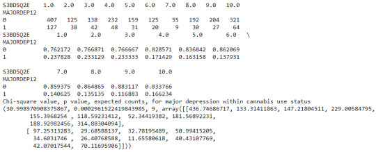
A Chi Square test of independence revealed that among cannabis users aged between 18 to 30 years old (susbetc2), the frequency of cannabis use (explanatory variable collapsed into 10 ordered categories) and past year depression diagnosis (response binary categorical variable) were significantly associated, X2 = 30.99,9 df, p=0.00029.

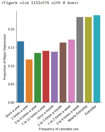
In the bivariate graph(C->C) presented above, we can see the correlation between frequency of cannabis use (explanatory variable) and major depression diagnosis in the past year (response variable). Obviously, we have a left-skewed distribution, which indicates that the more an individual (18-30) smoked cannabis, the better were the cases to have experienced depression in the last 12 months.

The post hoc comparison (Bonferroni Adjustment) of rates of major depression by the pair of “Every day” and “2 times a year” frequency categories, revealed that the p-value is 0.00019 and the percentages of major depression diagnosis for each frequency group are 23.7% and 11.6% respectively. As a result, since the p-value is smaller than the Bonferroni adjusted p-value (adj p-value = 0.05 / 45 = 0.0011>0.00019), we can assume that these two rates are significantly different from one another. Therefore, we reject the null hypothesis and accept the alternate. 

Similarly, the post hoc comparison (Bonferroni Adjustment) of rates of major depression by the pair of "1 or 2 times a week” and “2 times a year” frequency categories, indicated that the p-value is 0.107 and the proportions of major depression diagnosis for each frequency group are 17.1% and 11.6% respectively. As a result, since the p-value is larger than the Bonferroni adjusted p-value (adj p-value = 0.05 / 45 = 0.107>0.0011), we can assume that these two rates are not significantly different from one another. Therefore, we accept the null hypothesis.

[neeltron-blog]

Machine Learning for Data Analysis - Week 4 Assignment

Program

# -*- coding: utf-8 -*-

"""

Created on Tue Jun  9 06:40:12 2020

@author: Neel

"""

from pandas import pandas, DataFrame

import pandas as pd

import numpy as np

import matplotlib.pylab as plt

from sklearn.model_selection import train_test_split

from sklearn import preprocessing

from sklearn.cluster import KMeans

data = pd.read_csv("Data Management and Visualization/Mars Crater Dataset.csv")

data_clean = data.dropna()

cluster = data_clean[["LATITUDE_CIRCLE_IMAGE", "LONGITUDE_CIRCLE_IMAGE", "DEPTH_RIMFLOOR_TOPOG", "DIAM_CIRCLE_IMAGE"]]

print(cluster.describe())

clustervar = cluster.copy()

clustervar["LATITUDE_CIRCLE_IMAGE"] = preprocessing.scale(clustervar["LATITUDE_CIRCLE_IMAGE"].astype("float64"))

clustervar["LONGITUDE_CIRCLE_IMAGE"] = preprocessing.scale(clustervar["LONGITUDE_CIRCLE_IMAGE"].astype("float64"))

clustervar["DIAM_CIRCLE_IMAGE"] = preprocessing.scale(clustervar["DIAM_CIRCLE_IMAGE"].astype("float64"))

clustervar["DEPTH_RIMFLOOR_TOPOG"] = preprocessing.scale(clustervar["DEPTH_RIMFLOOR_TOPOG"].astype("float64"))

clus_train, clus_test = train_test_split(clustervar, test_size = 0.3, random_state = 123)

from scipy.spatial.distance import cdist

clusters = range(1, 10)

meandist = []

for k in clusters:

    model = KMeans(n_clusters = k)

    model.fit(clus_train)

    clus_assign = model.predict(clus_train)

    meandist.append(sum(np.min(cdist(clus_train, model.cluster_centers_, "euclidean"), axis = 1)) / clus_train.shape[0])

    plt.plot(clusters, meandist)

plt.xlabel("Number of Clusters")

plt.ylabel("Average distance")

plt.title("Selecting k with the elbow method")

model3 = KMeans(n_clusters = 4)

model3.fit(clus_train)

clusassign = model3.predict(clus_train)

from sklearn.decomposition import PCA

pca_3 = PCA(2)

plot_columns = pca_3.fit_transform(clus_train)

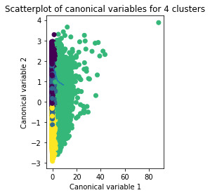
plt.scatter(x = plot_columns[:, 0], y = plot_columns[:, 1], c = model3.labels_,)

plt.xlabel("Canonical variable 1")

plt.ylabel("Canonical variable 2")

plt.title("Scatterplot of canonical variables for 4 clusters")

plt.show()

clus_train.reset_index(level = 0, inplace = True)

cluslist = list(clus_train['index'])

labels = list(model3.labels_)

newlist = dict(zip(cluslist, labels))

print(newlist)

newclus = DataFrame.from_dict(newlist, orient = "index")

print(newclus)

newclus.columns = ["cluster"]

newclus.reset_index(level = 0, inplace = True)

merged_train = pd.merge(clus_train, newclus, on = "index")

print(merged_train.head(n = 100))

merged_train.cluster.value_counts()

clustergrp = merged_train.groupby("cluster").mean()

print("Clustering variable means by cluster")

print(clustergrp)

layer_data = data_clean["NUMBER_LAYERS"]

layer_train, layer_test = train_test_split(layer_data, test_size = 0.3, random_state = 123)

layer_train1 = pd.DataFrame(layer_train)

layer_train1.reset_index(level = 0, inplace = True)

merged_train_all = pd.merge(layer_train1, merged_train, on = "index")

sub1 = merged_train_all[["NUMBER_LAYERS", "cluster"]].dropna()

import statsmodels.formula.api as smf

import statsmodels.stats.multicomp as multi

layermod = smf.ols(formula = "NUMBER_LAYERS ~ C(cluster)", data = sub1).fit()

print(layermod.summary())

print("means for number of layers by cluster")

m1 = sub1.groupby("cluster").mean()

print(m1)

print("standard deviations of number of layers by clusters")

s1 = sub1.groupby("cluster").std()

print(s1)

mc1 = multi.MultiComparison(sub1["NUMBER_LAYERS"], sub1["cluster"])

res1 = mc1.tukeyhsd()

print(res1.summary())

Output

       LATITUDE_CIRCLE_IMAGE  ...  DIAM_CIRCLE_IMAGE

count          384343.000000  ...      384343.000000

mean               -7.199209  ...           3.556686

std                33.608966  ...           8.591993

min               -86.700000  ...           1.000000

25%               -30.935000  ...           1.180000

50%               -10.079000  ...           1.530000

75%                17.222500  ...           2.550000

max                85.702000  ...        1164.220000

[8 rows x 4 columns]

15516   0

344967  1

172717  3

378336  1

346725  1

   ..

192476  0

17730   0

28030   0

277869  1

249342  2

[269040 rows x 1 columns]

     index  LATITUDE_CIRCLE_IMAGE  ...  DIAM_CIRCLE_IMAGE  cluster

0    15516               1.528797  ...          -0.259159        0

1   344967              -0.961762  ...          -0.297567        1

2   172717              -0.503015  ...          -0.287092        3

3   378336              -1.746048  ...          -0.235881        1

4   346725              -1.629978  ...           0.138887        1

..     ...                    ...  ...                ...      ...

95  153715              -0.058401  ...           0.062071        3

96  330653              -1.456780  ...          -0.295239        3

97   57613               1.591102  ...          -0.280108        0

98    6871               1.850348  ...           0.162164        0

99  256026              -0.029182  ...          -0.232390        1

[100 rows x 6 columns]

Clustering variable means by cluster

                 index  ...  DIAM_CIRCLE_IMAGE

cluster                 ...                   

0         69195.992176  ...          -0.149308

1        265614.659819  ...          -0.133282

2        201712.042174  ...           2.557181

3        239120.537881  ...          -0.141078

[4 rows x 5 columns]

                            OLS Regression Results                            

==============================================================================

Dep. Variable:          NUMBER_LAYERS   R-squared:                       0.120

Model:                            OLS   Adj. R-squared:                  0.120

Method:                 Least Squares   F-statistic:                 1.217e+04

Date:                Tue, 09 Jun 2020   Prob (F-statistic):               0.00

Time:                        22:54:30   Log-Likelihood:                -45298.

No. Observations:              269040   AIC:                         9.060e+04

Df Residuals:                  269036   BIC:                         9.065e+04

Df Model:                           3                                         

Covariance Type:            nonrobust                                         

===================================================================================

                      coef    std err          t      P>|t|      [0.025      0.975]

-----------------------------------------------------------------------------------

Intercept           0.0626      0.001     63.631      0.000       0.061       0.065

C(cluster)[T.1]    -0.0346      0.001    -25.021      0.000      -0.037      -0.032

C(cluster)[T.2]     0.4445      0.003    171.193      0.000       0.439       0.450

C(cluster)[T.3]    -0.0321      0.001    -22.965      0.000      -0.035      -0.029

==============================================================================

Omnibus:                   262358.235   Durbin-Watson:                   2.008

Prob(Omnibus):                  0.000   Jarque-Bera (JB):         12985631.133

Skew:                           4.851   Prob(JB):                         0.00

Kurtosis:                      35.623   Cond. No.                         5.47

==============================================================================

Warnings:

[1] Standard Errors assume that the covariance matrix of the errors is correctly specified.

means for number of layers by cluster

         NUMBER_LAYERS

cluster               

0             0.062638

1             0.028054

2             0.507146

3             0.030526

standard deviations of number of layers by clusters

         NUMBER_LAYERS

cluster               

0             0.290044

1             0.182880

2             0.803107

3             0.185748

Multiple Comparison of Means - Tukey HSD, FWER=0.05

====================================================

group1 group2 meandiff p-adj   lower   upper  reject

----------------------------------------------------

     0      1  -0.0346  0.001 -0.0381  -0.031   True

     0      2   0.4445  0.001  0.4378  0.4512   True

     0      3  -0.0321  0.001 -0.0357 -0.0285   True

     1      2   0.4791  0.001  0.4724  0.4857   True

     1      3   0.0025 0.2827 -0.0011   0.006�� False

     2      3  -0.4766  0.001 -0.4833 -0.4699   True

----------------------------------------------------

Graphs

Results

A k-means cluster analysis was conducted to identify underlying subgroups of craters based on their characteristics that could have an impact on their number of layers. Clustering variables included depth, diameter, latitude and longitude of the craters. All clustering variables were standardized to have a mean of 0 and a standard deviation of 1.

Data were randomly split into a training set that included 70% of the observations (N=11900) and a test set that included 30% of the observations (N=5100). A series of k-means cluster analyses were conducted on the training data specifying k=1-9 clusters, using Euclidean distance. The variance in the clustering variables that was accounted for by the clusters (r-square) was plotted for each of the nine cluster solutions in an elbow curve to provide guidance for choosing the number of clusters to interpret.

The elbow curve was inconclusive, suggesting that the 2, 4, 6 and 8-cluster solutions might be interpreted. The results below are for an interpretation of the 4-cluster solution.

The means on the clustering variables showed that, compared to the other clusters, craters in cluster 1 had moderate levels on the clustering variables. They had a relatively low likelihood of having second highest number of layers. Cluster 2 had the lowest levels of the number of layers. On the other hand, cluster 3 clearly included the most number of layers. Cluster 4 has the second lowest number of layers.

In order to externally validate the clusters, an Analysis of Variance (ANOVA) was conducted to test for significant differences between the clusters on the number of layers. A tukey test was used for post hoc comparisons between the clusters. Results indicated significant differences between the clusters on the number of layers. The tukey post hoc comparisons showed significant differences between clusters on number of layers, with the exception that clusters 1 and 3 were not significantly different from each other.

[2wowthings]

LINUX FILE SYSTEM

LINUX FILE SYSTEM

Linux File System (Directory Structure)

Linux is not the complete OS it is a number of packages built around a kernel. It has too many lines of code invented and developed by Mr. Linux Torvald in 1991. Developers can edit the code as it was released under open source and free for others.

The Linux file system is a mixture of folders or maybe directory. Everything in Linux is FILE. It is in form like a tree structure start with / directory. Each partition under the root directory.

TYPES OF LINUX FILE SYSTEM

ext2 Linux file System

ext3 

Linux file System

ext4 

Linux file System

JFS 

Linux file System

ReiserFS 

Linux file System

XFS 

Linux file System

btrfs 

Linux file System

swap 

Linux file System

ext2 Linux File System

ext2 stands for the second extended file system it was included in 1993.developed to overcome of limitation of the ext file system. It does not have a journaling feature. Maximum individual file size supports from 16 GB to 2 TB and overall ext2 file system size is 2 TB to 32 TB

ext3 Linux File System

ext3 stands for the third extended file system. Introduced in 2001 starting from Linux kernel 2.4.15 and onwards. The main benefit is to allow journalling. It is a dedicated area in the file system where all changes are tracked when the system crash the possibility of file system corruption is less because of the journaling feature. Maximum individual file size supports from 16 GB to 2 TB and overall ext3 file system size is 2 TB to 32 TB. Three types of journaling available in the ext3 file system.

          1 - Journal Metadata and content save in journal

          2 - Ordered Only metadata save in journal, metadata are journaled only after writing the content to disk and this is the default.

          3 - Writeback Only metadata save in journal. Metadata journaled either before or after the content is written to disk.

ext4 Linux File System

ext4 stands for fourth extended file system and it is introduced in 2008. Supports 64000 subdirectories in one directory. Maximum individual file size supports from 16 GB to 16 TB and overall ext4 file system size is 1 exabyte 

1 exabyte = 1024 PB

1 PB = 1024 TB

Here we have the option to switch off journalling features on or off.

JFS Linux file system

JFS is Journaled File System and developed by IBM. It can be an alternative to the EXT file system. 

ReiserFS Linux file system

ReiserFS is an alternative for the EXT3 file system. 

XFS Linux file system

XFS file system considered as high-speed JFS was developed for parallel I/O processing

btrfs Linux file system

btrfs file system is a b tree file system. using for fault tolerance, storage configuration, and many more. 

swap Linux file system

the swap file system is used for memory paging with equal to system RAM size 

LINUX FILE SYSTEM HIERARCHY 

ve Diagram explained itself about all directories 

Linux-file-systen

(Image Credit) Image Source - Google | Image By - Austinvernsonger

Few details of the above diagram  

/ directory ( root directory)

Everything on Linux located under the / directory also known as the root directory. It is similar to windows C:\ directory difference is Linux not having drive letters, on windows, it is D:\ but on Linux another partition under / directory 

/bin directory (user binaries)

This directory contains some of the standards commands of files. this may be useful for all the users also no special root or su permission required.

/sbin directory (system administration binaries)

/sbin directory is similar to the almost /bin directory. It contains essentials system administration commands files. Only run by root or super user.

/etc directory (configuration files)

This directory contains system configuration files. 

/dev directory (device file)

This directory contains device files. These all files associated with the device. Everything in Linux is a file.

/proc directory (kernel and process files)

This directory similar to /dev, It contains a special file that represents system and process information.

/var directory (variable data files)

This directory contains variable data files such as printing jobs.

/tmp directory (temporary files)

All the application store their temporary files in /tmp directory. these can be deleted after the system restarts.

/usr directory (user binaries and read-only data)

This contains user applications software files, libraries for a programming language, document files.

/home directory (users home directory)

This directory is having the home folder for each user created. This also contains users data files and user-specific configuration files 

/boot directory (boot files)

This directory contains Linux boot loader files

/lib directory (essentials shared libraries)

This directory contains libraries needed by essentials binaries in the /bin and /sbin directory 

/opt directory (optional package)

This directory contains subdirectories for optional software package

/mnt directory (temporary mount files)

This directory has system administrator temporary files mounted on /mnt 

/media directory (removable media)

This directory contains subdirectories where removable media device inserted into the computer are mounted 

/srv directory (service data)

It is having data for service provided by the system example website files under /srv (https server)

  We see working in details 

First, we check fdisk command here 

fdisk /dev/sda                  ( checking hard disk by using fdisk command)

We will get output like below 

command (m for help): p             (type p here for cheeking the details)

Gives us all partition details 

/dev/sda1

/dev/sda2

/dev/sda3

like this details about partitions

Now creating new partition we can use option n

type n and hit enter 

assigning cylinder value and partition size 

then save this partition with option w

now changing the partition type using option t

type t hit enter

now select partition number example 9 hit enter

type l for option 

83 is linux file system

type 83 and hit enter 

to check type p and hit enter 

type w for save and hit enter 

Now check fdisk -l /dev/sda     ( it will show us created partition)

The kernel must know this created partition so we use below command to update 

partprobe

and 

kpartx -a /dev/sda; kpartx -l /dev/sda

We can check cat /proc/partition the new partition in this way

CREATING FILE SYSTEM

mkfs.ext4 /dev/sda8       (using this command we define file system type)

OR

mke2fs -j -L data -b 2048 -i 4096 /dev/sda8

here are -L filesystem label

              -j journaling

              -b block size

              -i inode per every 4kb of disk space

LABELING TO LINUX FILE SYSTEM

e2label       

(Using this command we can give a name to file system)

e2label /dev/sda8 data    

(here we have give the name data to /dev/sda8)

If we want to use this new partition we need to mount the partition 

MOUNTING OF NEW LINUX FILE SYSTEM

mount LABEL=data /admin

TO CHECK LABELS AND TYPE OF ALL  FILE SYSTEM

blkid                       (This is the command we can check type of file system)

MANAGE PARAMETERS OF  LINUX FILE SYSTEM

dumpe2fs /dev/sda8             (this show all below details please check example)

file system flags

default mount option

block count

block size 

first block

inode count

last mounted on

UUID

file system magic number  

EXCLUDE FSCK CHECK FOR PARTICULAR LINUX FILE SYSTEM WHILE BOOTING 

tune2fs -i0 -c0 /dev/sda8     (this partition exclude while booting for fsck check purpose)

MOUNT POINT LINUX FILE SYSTEM

We will mount the partition in /etc/fstab file 

device                  mount point    fs type    options        dump_freq    fsck_order

LABEL=data       /admin             ext4       defaults             0                  0

Understand what is this mean

device                  device name 

mount point       path for using access to file system

fs type of file system

options                comma-separated list of different options can use

dump_freq          it is 1=daily, 2=every next day, 0=never dump

fsck_order           0=ignore and 1=first and from 2-9=second,third

             We can use command mount -a and check df -h for checking the mounted partition

DENY ACCESS TO PARTICULAR FOLDER OF LINUX FILE SYSTEM WHICH IS MOUNTED

mount -t ext4 -o noexec /dev/sda8 /admin

INCREASE I/O PERFORMANCE OF LINUX FILE SYSTEM

mount -t ext4 -o noatime /dev/sda8 /admin

UMOUNT LINUX FILE SYSTEM

We need to exit from partition and then need to use below command

umount /admin

CREATING SWAP PARTITION

fdisk -l /dev/sda

Check for the partition available or create using n command for new as we have discussed above 

mkswap /dev/sda10        (creating swap using mkswap the command for sda10)

Update in fstab

vim /etc/fstab

device                  mount point    fs type    options        dump_freq    fsck_order

/dev/sda10               swap             swap       defaults             0                  0

save this file and exit

Now 

swapon -a 

swapon -s 

CREATING SWAP FILE 

dd if=/dev/zero of=/swapfile bs=1024 count=100000  (will create swap file)

Now 

mkswap /swapfile

Update in fstab

device                  mount point    fs type    options        dump_freq    fsck_order

/swapfile               swap             swap         defaults             0                  0

save and exit the file 

swapon -a

swapon -s

Now we have created swap partition as well file 

This is LINUX FILE SYSTEM It is more in deep ANYTHING PLEASE CONTACT ME SUBSCRIBE FOR NEW UPDATES 

THANKS TO ALL GOD BLESS 

via Blogger https://ift.tt/3dWG2jY

[samthoughtjam]

Testing for Moderators using Python

Introduction:

This analysis uses a 2-factor ANOVA to test the influence of school level on how hobbies impact enjoyment in life. The school levels are: junior high school = grades 7-9 and senior high school = grades 10-12. In this test we examine if our explanatory variable is associated with our response level for each population sub-group (or each level of our third variable). Are hobby participation and enjoyment in life associated with those in grades 7-9 (junior HS)? And, are hobby participation and enjoyment in life associated with those in grades 10-12 (senior HS)? To answer these question I ran 2 ANOVA tests, one for each school or grade level.

Results for Grades 7-9 (junior high school):

When examining the association between enjoyment and hobby participation for those in grades 7-9 we see a high F-statistic of 21.87 and a very small p-value of 5.17e-14. When examining the means for this test we see hobbynum at enjoyment level 0 (rarely or never experience joy) at 1.84 while the highest levels of enjoyment (3 = enjoyment most or all the time) have a mean hobbynum of 3.06. The means show the levels of enjoyment increase with the amount of time spent on hobbies.

Results for Grades 10-12 (senior high school):

When examining the association between enjoyment and hobby participation for those in grades 10-12 we see an F-statistic of 7.63 and a small p-value of 4.40e-05. When examining the means for this test we see hobbynum at enjoyment level 0 (rarely or never experience joy) at 2.22 while the highest levels of enjoyment (3 = enjoyment most or all the time) have a mean hobbynum of 2.70. The means show the levels of enjoyment increase with the amount of time spent on hobbies, but the increase is lower than that experienced in grades 7-9.

Results Overall:

The school or grade level influence on the impact of hobbies on enjoyment in life is positive in both cases. However, the strength of the relationship is higher for grades 7-9. Though the p-values are statistically significant for both, the p-value is much smaller for the grades 7-9 (5.17e-14 vs. 4.40e-05) population and the associated F-statistic is larger (21.87 vs. 7.63). Therefore, school (or grade levels) moderate the relationship between the explanatory variable hobby participation and the response variable enjoyment in life. The junior high school or grades 7-9 group amplifies the relationship.

Selected Program Outputs:

         hobby     grade  hobbynum  gradenum enjoy                                         0      1.050725  8.036232  1.844203  8.036232 1      1.359031  8.121145  2.449339  8.121145 2      1.460157  8.078563  2.637486  8.078563 3      1.664780  7.998113  3.055031  7.998113

association between enjoyment and hobby participation for those in grades 7-9                            OLS Regression Results                             ============================================================================== Dep. Variable:               hobbynum   R-squared:                       0.021 Model:                            OLS   Adj. R-squared:                  0.020 Method:                 Least Squares   F-statistic:                     21.87 Date:                Sun, 19 Apr 2020   Prob (F-statistic):           5.17e-14 Time:                        12:35:23   Log-Likelihood:                -6736.8 No. Observations:                3073   AIC:                         1.348e+04 Df Residuals:                    3069   BIC:                         1.351e+04 Df Model:                           3                                         Covariance Type:            nonrobust                                         =================================================================================                    coef    std err          t      P>|t|      [0.025      0.975] --------------------------------------------------------------------------------- Intercept         1.8442      0.185      9.991      0.000       1.482       2.206 C(enjoy)[T.1]     0.6051      0.211      2.871      0.004       0.192       1.018 C(enjoy)[T.2]     0.7933      0.198      3.999      0.000       0.404       1.182 C(enjoy)[T.3]     1.2108      0.192      6.292      0.000       0.834       1.588 ============================================================================== Omnibus:                     3176.298   Durbin-Watson:                   2.020 Prob(Omnibus):                  0.000   Jarque-Bera (JB):              247.240 Skew:                           0.331   Prob(JB):                     2.05e-54 Kurtosis:                       1.778   Cond. No.                         11.4 ============================================================================== Warnings: [1] Standard Errors assume that the covariance matrix of the errors is correctly specified. association between enjoyment and hobby participation for those in grades 10-12                            OLS Regression Results                             ============================================================================== Dep. Variable:               hobbynum   R-squared:                       0.007 Model:                            OLS   Adj. R-squared:                  0.006 Method:                 Least Squares   F-statistic:                     7.633 Date:                Sun, 19 Apr 2020   Prob (F-statistic):           4.40e-05 Time:                        12:35:23   Log-Likelihood:                -7057.3 No. Observations:                3252   AIC:                         1.412e+04 Df Residuals:                    3248   BIC:                         1.415e+04 Df Model:                           3                                         Covariance Type:            nonrobust                                         =================================================================================                    coef    std err          t      P>|t|      [0.025      0.975] --------------------------------------------------------------------------------- Intercept         2.2176      0.204     10.866      0.000       1.817       2.618 C(enjoy)[T.1]     0.0192      0.223      0.086      0.931      -0.418       0.457 C(enjoy)[T.2]     0.2511      0.214      1.174      0.240      -0.168       0.670 C(enjoy)[T.3]     0.4784      0.211      2.263      0.024       0.064       0.893 ============================================================================== Omnibus:                      998.414   Durbin-Watson:                   1.999 Prob(Omnibus):                  0.000   Jarque-Bera (JB):              274.424 Skew:                           0.489   Prob(JB):                     2.57e-60 Kurtosis:                       1.965   Cond. No.                         13.0 ============================================================================== Warnings: [1] Standard Errors assume that the covariance matrix of the errors is correctly specified.

means for enjoyment by level of participation in hobbies for grades 7-9          hobby     grade  hobbynum  gradenum enjoy                                         0      1.050725  8.036232  1.844203  8.036232 1      1.359031  8.121145  2.449339  8.121145 2      1.460157  8.078563  2.637486  8.078563 3      1.664780  7.998113  3.055031  7.998113

means for enjoyment by level of participation in hobbies for grades 10-12          hobby      grade  hobbynum   gradenum enjoy                                           0      1.250000  10.796296  2.217593  10.796296 1      1.254083  10.976407  2.236842  10.976407 2      1.379873  10.965549  2.468722  10.965549 3      1.487248  10.951007  2.695973  10.951007

Source Code:

import pandas as pd import os import statsmodels.formula.api as smf

def grade_school(row):    """    used to create a variable coded 1 for high school (10-12) and 0 for junior high school (7-9)    :param row: series - dataset row    :return: int - 1 for highlest level of life enjoyment (3), 0 for anything less (0, 1, 2)    """    if row["gradenum"] < 10:        return 0    else:        return 1

# set path and filename for the data file and load the dataset data_file = os.path.join(os.path.dirname(os.path.realpath(__file__)) + "\\data", "addhealth_pds.csv") data = pd.read_csv(data_file, low_memory=False) # create a small dataframe containing only the variables of interest df = pd.DataFrame({"hobby": data["H1DA2"], "enjoy": data["H1FS15"], "grade": data["H1GI20"]})

# HOBBY variable - explanatory variable # remove the missing value rows (values 6 and 8) df = df[df["hobby"] < 4] # convert the hobby value to a small integer df["hobby"] = pd.to_numeric(pd.Series(df["hobby"]), errors="coerce") # change format from numeric to categorical # recoding number of days smoked in the past month recode1 = {0: 0, 1: 1.5, 2: 3.5, 3: 6} df['hobbynum']= df['hobby'].map(recode1) print("For the quantitative variable hobbynum show descriptive statistics:") print(df["hobbynum"].describe())

# ENJOY variable - response variable # remove the missing value rows (values 6 and 8) df = df[df["enjoy"] < 4] # convert the happy value into a small integer df["enjoy"] = pd.to_numeric(pd.Series(df["enjoy"]), downcast="signed", errors="coerce") # change format from numeric to categorical df["enjoy"] = df["enjoy"].astype('category') print("For the categorical variable enjoy show the total count, unique categories, top category, and top count:") print(df["enjoy"].describe())

# GRADE variable # remove the missing value rows (values 96-99) df = df[df["grade"] < 13] # convert the grade value to a small integer df["gradenum"] = pd.to_numeric(pd.Series(df["grade"]), downcast="signed", errors="coerce") print("For the quantitative variable gradenum show descriptive statistics:") print(df["gradenum"].describe())

# School variable - moderator - grade 7-9 = junior high and grade 10-12 senior HS df["school"] = df.apply(lambda row: grade_school(row), axis=1) # change format from numeric to categorical df["school"] = df["school"].astype('category') print("For the categorical variable school show the total count, unique categories, top category, and top count:") print(df["school"].describe())

sub2 = df[(df['school'] == 0)] sub3 = df[(df['school'] == 1)]

print('association between enjoyment and hobby participation for those in grades 7-9') model2 = smf.ols(formula='hobbynum ~ C(enjoy)', data=sub2).fit() print(model2.summary())

print('association between enjoyment and hobby participation for those in grades 10-12') model3 = smf.ols(formula='hobbynum ~ C(enjoy)', data=sub3).fit() print(model3.summary())

print("means for enjoyment by level of participation in hobbies for grades 7-9") m3 = sub2.groupby('enjoy').mean() print(m3)

print("means for enjoyment by level of participation in hobbies for grades 10-12") m4 = sub3.groupby('enjoy').mean() print(m4)

[uspscourse]

Data Analyst 2v2

1) Program: Gapminder2v2.py

import pandas import numpy import scipy.stats import statsmodels.formula.api as sf_api import seaborn import matplotlib.pyplot as plt

""" any additional libraries would be imported here """

""" Set PANDAS to show all columns in DataFrame """ pandas.set_option('display.max_columns', None)

"""Set PANDAS to show all rows in DataFrame """ pandas.set_option('display.max_rows', None)

""" bug fix for display formats to avoid run time errors """ pandas.set_option('display.float_format', lambda x:'%f'%x)

""" read in csv file """ data = pandas.read_csv('gapminder.csv', low_memory=False) data = data.replace(r'^\s*$', numpy.NaN, regex=True)

""" checking the format of your variables """ data['country'].dtype

""" setting variables you will be working with to numeric """ data['employrate'] = pandas.to_numeric(data['employrate'], errors='coerce') data['internetuserate'] = pandas.to_numeric(data['internetuserate'], errors='coerce') data['lifeexpectancy'] = pandas.to_numeric(data['lifeexpectancy'], errors='coerce')

"""  subset of employrate less than 76 percent, internetuserate between  25 - 75 percent and lifeexpectancy between 50 - 75 years   """ sub1=data[(data['employrate'] <= 75) & (data['lifeexpectancy'] > 50) \     & (data['lifeexpectancy'] <= 75) & (data['internetuserate'] > 50) \     & (data['internetuserate'] <= 75)]

""" make a copy of subset data 1 """ sub2=sub1.copy()

""" recoding - replace NaN to 0 and recoding to interger """ sub2['employrate'].fillna(0, inplace=True) sub2['internetuserate'].fillna(0, inplace=True) sub2['lifeexpectancy'].fillna(0, inplace=True) sub2['employrate']=sub1['employrate'].astype(int) sub2['internetuserate']=sub1['internetuserate'].astype(int) sub2['lifeexpectancy']=sub1['lifeexpectancy'].astype(int)

""" recode quantitative variable to categorical to practice chi-square  """ sub2['employrate'].astype('category') sub2['internetuserate'].astype('category')

""" use ols function for F-statistic and associated p-value """ model_a = sf_api.ols(formula='employrate ~ C(internetuserate)', data=sub2).fit() print(model_a.summary())

sub3=sub2[['employrate', 'internetuserate']].dropna().astype(int)

""" contingency table of observed counts """ print("contingency table of observed counts") oc=pandas.crosstab(sub3['employrate'], sub3['internetuserate']) print(oc)

""" column percentages """ colpct=oc/oc.sum(axis=0) print("column percentages of contingency table") print(colpct)

""" chi-square test of independence """ print("chi-square, p value, expected counts") cs=scipy.stats.chi2_contingency(oc) print(cs)

2) Output: Chi-Square Test of Independence

                           OLS Regression Results                             ============================================================================== Dep. Variable:             employrate   R-squared:                       1.000 Model:                            OLS   Adj. R-squared:                    nan Method:                 Least Squares   F-statistic:                       nan Date:                Fri, 26 Feb 2021   Prob (F-statistic):                nan Time:                        18:03:05   Log-Likelihood:                 219.29 No. Observations:                   7   AIC:                            -424.6 Df Residuals:                       0   BIC:                            -425.0 Df Model:                           6                                         Covariance Type:            nonrobust                                         ============================================================================================                               coef    std err          t      P>|t|      [0.025      0.975] -------------------------------------------------------------------------------------------- Intercept                   34.0000        inf          0        nan         nan         nan C(internetuserate)[T.56]    26.0000        inf          0        nan         nan         nan C(internetuserate)[T.61]    16.0000        inf          0        nan         nan         nan C(internetuserate)[T.62]    19.0000        inf          0        nan         nan         nan C(internetuserate)[T.65]    13.0000        inf          0        nan         nan         nan C(internetuserate)[T.71]    22.0000        inf          0        nan         nan         nan C(internetuserate)[T.74]    22.0000        inf          0        nan         nan         nan ============================================================================== Omnibus:                          nan   Durbin-Watson:                   1.400 Prob(Omnibus):                    nan   Jarque-Bera (JB):                0.749 Skew:                          -0.272   Prob(JB):                        0.688 Kurtosis:                       1.493   Cond. No.                         7.87 ==============================================================================

Notes: [1] Standard Errors assume that the covariance matrix of the errors is correctly specified. contingency table of observed counts internetuserate  51  56  61  62  65  71  74 employrate                                 34                1   0   0   0   0   0   0 47                0   0   0   0   1   0   0 50                0   0   1   0   0   0   0 53                0   0   0   1   0   0   0 56                0   0   0   0   0   1   1 60                0   1   0   0   0   0   0 column percentages of contingency table internetuserate       51       56       61       62       65       71       74 employrate                                                                     34              1.000000 0.000000 0.000000 0.000000 0.000000 0.000000 0.000000 47              0.000000 0.000000 0.000000 0.000000 1.000000 0.000000 0.000000 50              0.000000 0.000000 1.000000 0.000000 0.000000 0.000000 0.000000 53              0.000000 0.000000 0.000000 1.000000 0.000000 0.000000 0.000000 56              0.000000 0.000000 0.000000 0.000000 0.000000 1.000000 1.000000 60              0.000000 1.000000 0.000000 0.000000 0.000000 0.000000 0.000000 chi-square, p value, expected counts (35.000000000000014, 0.24264043734973734, 30, array([       [0.14285714, 0.14285714, 0.14285714, 0.14285714, 0.14285714,        0.14285714, 0.14285714],       [0.14285714, 0.14285714, 0.14285714, 0.14285714, 0.14285714,        0.14285714, 0.14285714],       [0.14285714, 0.14285714, 0.14285714, 0.14285714, 0.14285714,        0.14285714, 0.14285714],       [0.14285714, 0.14285714, 0.14285714, 0.14285714, 0.14285714,        0.14285714, 0.14285714],       [0.28571429, 0.28571429, 0.28571429, 0.28571429, 0.28571429,        0.28571429, 0.28571429],       [0.14285714, 0.14285714, 0.14285714, 0.14285714, 0.14285714,        0.14285714, 0.14285714]]))

3) Testing the variables employrate and internetuserate of countries with under 75% employ rate and between 50 - 75% internet use rate which I convert from quantitative to categorical and float to interger for this exercise. I produced the contingency table (in percentage form as well) of observed counts and the chi-square, p value and expected counts for this effort (see output on item two for more details)

[rmjddvm]

Program and output

**********PROGRAM**********

# -*- coding: utf-8 -*- """ Created on Thu Apr 16 00:48:12 2020

@author: juan.viramontes """

import numpy as np import pandas as pd import seaborn as sns import statsmodels.api as sm import statsmodels.formula.api as smf data = pd.read_csv('gapmod.csv') print("\n"*2) print("*****Informacion*****") print(data.info()) print("\n"*2) print("*****Primeros datos*****") print(data.head()) print("\n"*2) print("*****Estadisticos iniciales*****") print(data.describe()) sns.lmplot('urbanrate', 'lifeexpectancy', data=data) print("\n"*2) print('OLS regression model for association between urban rate and life expectancy') reg1=smf.ols('lifeexpectancy ~ urbanrate',data=data).fit() print(reg1.summary()) mean_ur=np.mean(data.urbanrate) print("\n"*2) print("*****Urbanrate Mean*****") print(mean_ur) print("\n"*2) print("*****Estadisticos iniciales de urbanrate_norm*****") data['urbanrate_norm']=data['urbanrate']-mean_ur print(data.head()) print(data.describe()) print("\n"*2) sns.lmplot('urbanrate_norm', 'lifeexpectancy', data=data) reg1=smf.ols('lifeexpectancy ~ urbanrate_norm',data=data).fit() print(reg1.summary()) mean_ur_norm=np.mean(data.urbanrate_norm) print("\n"*2) print("*****Urbanrate_norm Mean*****") print(mean_ur_norm) #N_Col=data.urbanrate-mean_ur #print(N_Col)

*********OUTPUT**********

Python 3.7.6 (default, Jan  8 2020, 20:23:39) [MSC v.1916 64 bit (AMD64)] Type "copyright", "credits" or "license" for more information.

IPython 7.12.0 -- An enhanced Interactive Python.

Reiniciando el núcleo...

runfile('C:/Users/juan.viramontes/.spyder-py3/Tarea2.py', wdir='C:/Users/juan.viramontes/.spyder-py3')

*****Informacion***** <class 'pandas.core.frame.DataFrame'> RangeIndex: 176 entries, 0 to 175 Data columns (total 4 columns): #   Column           Non-Null Count  Dtype   ---  ------           --------------  -----   0   country          176 non-null    object 1   incomeperperson  176 non-null    float64 2   lifeexpectancy   176 non-null    float64 3   urbanrate        176 non-null    float64 dtypes: float64(3), object(1) memory usage: 5.6+ KB None

*****Primeros datos*****     country  incomeperperson  lifeexpectancy  urbanrate 0    Albania          1915.00          76.918      46.72 1    Algeria          2231.99          73.131      65.22 2     Angola          1381.00          51.093      56.70 3  Argentina         10749.42          75.901      92.00 4    Armenia          1326.74          74.241      63.86

*****Estadisticos iniciales*****       incomeperperson  lifeexpectancy   urbanrate count       176.000000      176.000000  176.000000 mean       7327.444261       69.654733   55.566364 std       10567.303760        9.729521   23.225708 min         103.780000       47.794000   10.400000 25%         702.367500       63.041500   36.685000 50%        2385.185000       73.126500   56.970000 75%        8497.782500       76.569500   73.465000 max       52301.590000       83.394000  100.000000

OLS regression model for association between urban rate and life expectancy                            OLS Regression Results                             ============================================================================== Dep. Variable:         lifeexpectancy   R-squared:                       0.378 Model:                            OLS   Adj. R-squared:                  0.374 Method:                 Least Squares   F-statistic:                     105.7 Date:                Thu, 16 Apr 2020   Prob (F-statistic):           1.14e-19 Time:                        15:49:12   Log-Likelihood:                -607.90 No. Observations:                 176   AIC:                             1220. Df Residuals:                     174   BIC:                             1226. Df Model:                           1                                         Covariance Type:            nonrobust                                         ==============================================================================                 coef    std err          t      P>|t|      [0.025      0.975] ------------------------------------------------------------------------------ Intercept     55.3458      1.508     36.703      0.000      52.370      58.322 urbanrate      0.2575      0.025     10.280      0.000       0.208       0.307 ============================================================================== Omnibus:                       13.445   Durbin-Watson:                   1.891 Prob(Omnibus):                  0.001   Jarque-Bera (JB):               14.888 Skew:                          -0.712   Prob(JB):                     0.000585 Kurtosis:                       3.005   Cond. No.                         157. ==============================================================================

Warnings: [1] Standard Errors assume that the covariance matrix of the errors is correctly specified.

*****Urbanrate Mean***** 55.56636363636364

*****Estadisticos iniciales de urbanrate_norm*****     country  incomeperperson  lifeexpectancy  urbanrate  urbanrate_norm 0    Albania          1915.00          76.918      46.72       -8.846364 1    Algeria          2231.99          73.131      65.22        9.653636 2     Angola          1381.00          51.093      56.70        1.133636 3  Argentina         10749.42          75.901      92.00       36.433636 4    Armenia          1326.74          74.241      63.86        8.293636       incomeperperson  lifeexpectancy   urbanrate  urbanrate_norm count       176.000000      176.000000  176.000000    1.760000e+02 mean       7327.444261       69.654733   55.566364   -3.593085e-15 std       10567.303760        9.729521   23.225708    2.322571e+01 min         103.780000       47.794000   10.400000   -4.516636e+01 25%         702.367500       63.041500   36.685000   -1.888136e+01 50%        2385.185000       73.126500   56.970000    1.403636e+00 75%        8497.782500       76.569500   73.465000    1.789864e+01 max       52301.590000       83.394000  100.000000    4.443364e+01

                           OLS Regression Results                             ============================================================================== Dep. Variable:         lifeexpectancy   R-squared:                       0.378 Model:                            OLS   Adj. R-squared:                  0.374 Method:                 Least Squares   F-statistic:                     105.7 Date:                Thu, 16 Apr 2020   Prob (F-statistic):           1.14e-19 Time:                        15:49:13   Log-Likelihood:                -607.90 No. Observations:                 176   AIC:                             1220. Df Residuals:                     174   BIC:                             1226. Df Model:                           1                                         Covariance Type:            nonrobust                                         ==================================================================================                     coef    std err          t      P>|t|      [0.025      0.975] ---------------------------------------------------------------------------------- Intercept         69.6547      0.580    120.069      0.000      68.510      70.800 urbanrate_norm     0.2575      0.025     10.280      0.000       0.208       0.307 ============================================================================== Omnibus:                       13.445   Durbin-Watson:                   1.891 Prob(Omnibus):                  0.001   Jarque-Bera (JB):               14.888 Skew:                          -0.712   Prob(JB):                     0.000585 Kurtosis:                       3.005   Cond. No.                         23.2 ==============================================================================

Warnings: [1] Standard Errors assume that the covariance matrix of the errors is correctly specified.

*****Urbanrate_norm Mean***** -3.593085425150507e-15

[essayyard-blog]

Programming Question Part 1ProblemDevelop a simple Python program to demonstrate understanding of using the

New Post has been published on https://www.essayyard.com/programming-question-part-1problemdevelop-a-simple-python-program-to-demonstrate-understanding-of-using-the/

Programming Question Part 1ProblemDevelop a simple Python program to demonstrate understanding of using the

Part 1ProblemDevelop a simple Python program to demonstrate understanding of using the Tkinter module to design a simple widget and configure it using the layout manager. Then add an event handler that will accept text input to the button and display the content of the text when using the mouse to click on the “click here” button.The program must have the following:Documentation Guidelines:Use good programming style (e.g., indentation for readability) and document each of your program parts with the following items (the items shown between the ” angle brackets are only placeholders. You should replace the placeholders and the comments between them with your specific information). Your cover sheet should have some of the same information, but what follows should be at the top of each program’s sheet of source code. Some lines of code should have an explanation of what is to be accomplished, this will allow someone supporting your code years later to comprehend your purpose. Be brief and to the point. Start your design by writing comment lines of pseudocode. Once that is complete, begin adding executable lines. Finally run and test your program.Deliverable(s):Your deliverable should be a Word document with screenshots showing the source code and running results, and discuss the issues that you had for this project related to AWS and/or Python IDE and how you solved them for all of the programs listed above as well as the inputs and outputs from running them. Submit a cover sheet with the hardcopy of your work.part 2For this assignment, you will develop working examples of a graphical user interface (GUI) and event handling and that demonstrate the following:Be sure to include a brief narrative of your code where you explain what the code is doing.Documentation Guidelines:Use good programming style (e.g., indentation for readability) and document each of your program parts with the following items (the items shown between the ” angle brackets are only placeholders. You should replace the placeholders and the comments between them with your specific information). Your cover sheet should have some of the same information, but what follows should be at the top of each program’s sheet of source code. Some lines of code should have an explanation of what is to be accomplished, this will allow someone supporting your code years later to comprehend your purpose. Be brief and to the point. Start your design by writing comment lines of pseudocode. Once that is complete, begin adding executable lines. Finally run and test your program.Deliverable(s):Your deliverable should be a Word document with screenshots showing the GUI and event handling you have created. Also, discuss the issues that you had for this project related to AWS and/or Python IDE and how you solved them for all of the programs listed above as well as the inputs and outputs from running them. Submit a cover sheet with the hardcopy of your work.Part 3Write a Python program using the Python IDE based on recursion with trees that is both depth first and breadth first searches.The Python program to be developed will demonstrate the use of both depth-first (DFS) and breadth-first (BFS) searches. A tree node structure will be developed that will be used both for DFS and BFS searches. The program will apply recursion both for the DFS and BFS searches to completion of the entire DFS and BFS. Also, the Python program will provide as output some of the intermediate nodes that are transverse during the execution of the DFS and BFS. This output of the intermediate nodes searched will demonstrate the different paths executed during a DFS versus BFS.ProblemDevelop functions to demonstrate understanding of implementing a recursive depth first search (DFS) and an iterative breadth first search (BFS) in Python using a simple graph made of nodes. This example will use nodes A, B, C, D, and E connected as follows: A —– / | B-D-C | | / | E —–The program must have the following:Documentation Guidelines:Use good programming style (e.g., indentation for readability) and document each of your program parts with the following items (the items shown between the ” angle brackets are only placeholders. You should replace the placeholders and the comments between them with your specific information). Your cover sheet should have some of the same information, but what follows should be at the top of each program’s sheet of source code. Some lines of code should have an explanation of what is to be accomplished, this will allow someone supporting your code years later to comprehend your purpose. Be brief and to the point. Start your design by writing comment lines of pseudocode. Once that is complete, begin adding executable lines. Finally run and test your program.Deliverable(s):Your deliverable should be a Word document with screenshots showing the source code and running results, and discuss the issues that you had for this project related to AWS and/or Python IDE and how you solved them for all of the programs listed above as well as the inputs and outputs from running them. Submit a cover sheet with the hardcopy of your work.Part 4Two user-defined classes are recommended: class Transaction, and class BankStatement. A main() function will be required that declares a BankStatement object and Transaction objects and then performs operations as shown in the example driver main function below. The BankStatement object (called myStatement in the example main() shown later) contains a container of Transaction objects along with other record-keeping data fields. This is yet another example of the Containment/Composition (a.k.a., “Has-A”) relationship that can exist between classes/objects.The Transaction class is used to create deposit and withdrawal objects. It contains a constructor for initialization. This constructor has three defaulted parameters to facilitate the user declaring transactions and passing appropriate initial data member values as parameters to this constructor or accepting one or more of its defaulted initializer values. It is certainly legal, and perhaps desirable, to also have a LoadTransaction() method that would take inputs from the keyboard on an interactive basis. This, in conjunction with a menu, is a desirable addition but not required for this exercise. The main() driver function shows a partial batch (i.e., hard-coded) implementation rather than the, perhaps, more desirable interactive implementation. See your instructor for any specific additional requirements.# Python model of a bank transaction which can be either# A deposit or a withdraw## Filename: transaction.pyclass Transaction: def __init__(self, inAmount = 0.0, inCode = ‘D’, inNote = “No note”): self.__Amount = inAmount if inAmount >= 0.0 else 0.0 self.__Code = inCode if inCode == ‘D’ or inCode == ‘W’ else ‘D’ self.__Note = inNote if len(inNote) > 0 else “No note” def setAmount(self, newAmount): self.__Amount = newAmount if newAmount >= 0.0 else self.__Amount def getAmount(self): return self.__Amount def setCode(self, newCode): self.__Code = newCode if newCode == ‘W’ or newCode == ‘D’ else self.__Code def getCode(self): return self.__Code def setNote(self, newNote): self.__Note = newNote if len(newNote) > 0 else self.__Note def getNote(self): return self.__Note def loadTransaction(self): self.setAmount(float(input(“Enter transaction amount(DD.CC), $ “))) self.setCode(input(“Enter transaction code (‘W’ or ‘D’), “)) self.setNote(input(“Enter purpose of transaction, “))The BankStatement class contains two list containers of Transaction objects, a list container of float values, some BankStatement support data fields, and the required methods to manipulate selected data fields, insert transactions, arrange (i.e., sort) the contained transaction objects, and print them.# Python model of a bank statement capable of# holding and managing multiple bank transactions## Filename: bankStatement.pyfrom transaction import Transactionclass BankStatement: def __init__(self, begBal = 0.0, endBal = 0.0): self.__TransactionLog = [] self.__ArrangedLog = [] self.__RunningBalLog = [] self.__BegBal = begBal self.__EndBal = endBal self.__NumEntries = 0 self.__NumDeposits = 0 self.__NumWithdrawals = 0 def setBegEndBals(self, balance): self.__BegBal = self.__EndBal = balance def getBegBal(self): return self.__BegBal def getEndBal(self): return self.__EndBal def getNumEntries(self): return self.__NumEntries def getNumDeposits(self): return self.__NumDeposits def getNumWithdrawals(self): return self.__NumWithdrawals def insertTransaction(self, transaction): self.__Transactionlog.append(transaction) # Update __RunningBalLog, increment __NumEntries and increment either # __NumDeposits or __NumWithdrawals depending upon whether transaction is a deposit # or a withdrawal def displayResults(self): # Displays __BegBal, __TransactionLog list, __RunningBal list, and final stats (i.e., __EndBal, total transactions, number of deposits and number of withdrawls) # See example output def arrangeTransactions(self): # Builds __ArrangedLog list from __TransactionLog list def printArranged(self): # Displays the __ArrangedLog listThe declared classes and their contents are a starting point for the program. You may not need all the class members described above. Do not feel bound to implement this program using the exact methods and/or data fields given. The primary objective is for you to solve the problem of providing a bank statement to the bank’s customers using O-O programming techniques. HOWEVER, if you deviate from the above design be sure to fully document your design! If in doubt as to whether your deviation violates the intent of this exercise, ask your instructor.In the interest of sound software engineering practice, make sure to validate the values provided to the constructor method of class BankStatement. For invalid values you may choose to completely reject the passed in values and set the data fields to some default (but valid) values. In either case you should also display an error message.Below is a non-interactive(i.e., batch), main driver test function that will confirm to you and your instructor that the program operates as expected. Use the transaction objects given as data for your final submission of the program.def main(): # NOTE THIS IS A NON-INTERACTIVE DRIVER! myStatement = BankStatement() myStatement.setBegEndBals(15.92); # Sets beginning AND ending balance data fields # Declare some transaction objects T1 = Transaction() # TEST DATA T1.setAmount (123.56) T1.setCode(‘D’) T1.setNote(“CTPay”) T2 = Transaction(153.86, ‘W’,”Rent”) T3 = Transaction() T3.setAmount(75.56) T3.setCode(‘D’) T3.setNote(“Tips”) T4 = Transaction(12.56, ‘D’,”Gift”) T5 = Transaction() T5.setAmount(73.74) T5.setCode(‘W’) T5.setNote(“Date”) T6 = Transaction(145.75, ‘D’,”Loan”) T7 = Transaction() T7.setAmount(40.00) T7.setCode(‘W’) T7.setNote(“Loan Payment”) T8 = Transaction(21.74, ‘W’, “Groceries”) # Now insert the transaction objects into the bank statement myStatement.enterTransaction(T1) # Enter transactions into the myStatement.enterTransaction(T2) # BankStatement object # Six more transactions entered…………………………………………………………… ……………………………………………………………………………………………… # continue # Manipulate the bank statement myStatement.displayResults() myStatement.arrangeTransactions() myStatement.printArranged()The following is a look at what the output might look like from the method, displayResults(). The beginning balance was: $15.92 Transaction: 1 was a D amount: $123.56 for CTPay Running Bal: $139.48 Transaction: 2 was a W amount: $153.86 for Rent Running Bal: $-14.38 OVERDRAWN etc., for the other transactions……….…………………………………………………… …….………………………………………………………………………………………. The ending balance is: $84.01 The number of Transactions is: 8 The number of Deposits is: 4 The number of Withdrawals is: 4The following is the result after calling the arrangeTransactions() and printArranged() methods in the BankStatement class. Printing the Deposits and Withdrawals as a group: Transaction was a D amount: $123.56 for CTPay Transaction was a D amount: $75.56 for Tips Transaction was a D amount: $12.56 for Gift Transaction was a D amount: $145.75 for Loan Transaction was a W amount: $153.86 for Rent Transaction was a W amount: $73.74 for Date Transaction was a W amount:$40.00 for Loan Payment Transaction was a W amount: $21.74 for GroceriesTo build the ArrangedLog container in method, arrangeTransactions(), the following strategy is recommended: 1. Traverse the TransactionLog container checking each cell to determine if it is a deposit (‘D’) or withdrawal (‘W’): Loop for number of entries in the TransactionLog if TransactionLog[i].getCode() == ‘D’: append transaction in TransactionLog[i] to next open cell in list container, ArrangedLog 2. In another loop (very similar to the loop above), go back to the beginning of the TransactionLog container and check for all the ‘W’s and copy (i.e., append) them to the ArrangedLog container following the deposits.Now the method, printArranged(), just needs to loop through its entries and display the contents of the ArrangedLog container as shown above.Notice that the methods of an object contained within a containment object are accessed with the selection operator just as though you had the name of the object. However, inside the BankStatement object (myStatement), all you have access to is a container of Transaction objects — not their individual names — hence the TransactionLog[i].getNote() notation.Deliverable(s)Your deliverable should be a Word document with screenshots showing the source code and running results. If the source code is too long, you may insert your source code files as Packages into the Word document. You may also login to the class by using a browser in the AWS, and upload your source code directly. Submit a cover sheet with the hardcopy of your work.

[hellodatascientist-blog]

Coursera Data Analysis Tools HW1

Program:

import pandas import numpy import re import statsmodels.formula.api as smf import statsmodels.stats.multicomp as multi # any additional libraries would be imported here

data = pandas.read_csv('nesarc_pds.csv', low_memory=False)

print (len(data)) #number of observations (rows) print (len(data.columns)) # number of variables (columns)

codebook = ''' # S2AQ8A HOW OFTEN DRANK ANY ALCOHOL IN LAST 12 MONTHS # S2AQ8B NUMBER OF DRINKS OF ANY ALCOHOL USUALLY CONSUMED ON DAYS WHEN DRANK ALCOHOL IN LAST 12 MONTHS # S2AQ8C LARGEST NUMBER OF DRINKS OF ANY ALCOHOL CONSUMED ON DAYS WHEN DRANK ALCOHOL IN LAST 12 MONTHS # S2AQ8D HOW OFTEN DRANK LARGEST NUMBER OF DRINKS OF ANY ALCOHOL IN LAST 12 MONTHS # S2AQ8E HOW OFTEN DRANK 5+ DRINKS OF ANY ALCOHOL IN LAST 12 MONTHS # S2AQ9 HOW OFTEN DRANK 4+ DRINKS OF ANY ALCOHOL IN LAST 12 MONTHS (WOMEN ONLY) # S2AQ10 HOW OFTEN DRANK ENOUGH TO FEEL INTOXICATED IN LAST 12 MONTHS # S2AQ11 HOW MANY DRINKS CAN HOLD WITHOUT FEELING INTOXICATED # S2AQ4B HOW OFTEN DRANK COOLERS IN LAST 12 MONTHS # S2AQ5B HOW OFTEN DRANK BEER IN LAST 12 MONTHS # S2AQ6B HOW OFTEN DRANK WINE IN LAST 12 MONTHS # S2AQ7B HOW OFTEN DRANK LIQUOR IN LAST 12 MONTHS # S2AQ14 NUMBER OF YEARS DRANK SAME AS IN LAST 12 MONTHS # S2AQ15R1 NUMBER OF MONTHS SINCE LAST DRINK (ROUNDED TO NEAREST MONTH) # S2AQ16A AGE WHEN STARTED DRINKING, NOT COUNTING SMALL TASTES OR SIPS # S2AQ19 AGE AT START OF PERIOD OF HEAVIEST DRINKING # S2AQ20 DURATION (YEARS) OF PERIOD OF HEAVIEST DRINKING # S2AQ21A HOW OFTEN DRANK ANY ALCOHOL DURING PERIOD OF HEAVIEST DRINKING # S2AQ21B NUMBER OF DRINKS OF ANY ALCOHOL USUALLY CONSUMED ON DAYS WHEN DRANK ALCOHOL DURING PERIOD OF HEAVIEST DRINKING # S2AQ21C LARGEST NUMBER OF DRINKS OF ANY ALCOHOL CONSUMED ON DAYS WHEN DRANK ALCOHOL DURING PERIOD OF HEAVIEST DRINKING # S2AQ21D HOW OFTEN DRANK LARGEST NUMBER OF DRINKS OF ANY ALCOHOL DURING PERIOD OF HEAVIEST DRINKING # S2AQ22 HOW OFTEN DRANK 5+ DRINKS OF ANY ALCOHOL DURING PERIOD OF HEAVIEST DRINKING # S2AQ23 MAIN TYPE OF ALCOHOL CONSUMED DURING PERIOD OF HEAVIEST DRINKING # S2DQ1 BLOOD/NATURAL FATHER EVER AN ALCOHOLIC OR PROBLEM DRINKER # S2DQ2 BLOOD/NATURAL MOTHER EVER AN ALCOHOLIC OR PROBLEM DRINKER # S2DQ3C2 ANY FULL BROTHERS EVER ALCOHOLICS OR PROBLEM DRINKERS # S2DQ4C2 ANY FULL SISTERS EVER ALCOHOLICS OR PROBLEM DRINKERS # S2DQ5C2 ANY NATURAL SONS EVER ALCOHOLICS OR PROBLEM DRINKERS # S2DQ6C2 ANY NATURAL DAUGHTERS EVER ALCOHOLICS OR PROBLEM DRINKERS ''' #extract code and description m = re.findall(r'^# (\w+) (.*)$', codebook, re.MULTILINE)

#build code to description map code_dict = {} for code in m:    code_dict[code[0]] = code[1]

#setting variables you will be working with to numeric for code in m:    data[code[0]].replace(r'\s+', numpy.nan, regex=True, inplace=True)    data[code[0]] = pandas.to_numeric(data[code[0]])

data['S2AQ8C'] = data['S2AQ8C'].replace(99, numpy.nan) data['S2DQ1'] = data['S2DQ1'].replace(9, numpy.nan)

data['S2DQ1'] = pandas.Categorical(data.S2DQ1) data['S2DQ1']=data['S2DQ1'].cat.rename_categories(['Yes', 'No'])

# using ols function for calculating the F-statistic and associated p value model1 = smf.ols(formula='S2AQ8C ~ C(S2DQ1)', data=data) results1 = model1.fit() print(results1.summary())

sub1 = data[['S2AQ8C', 'S2DQ1']].dropna()

print('means for {0} by {1}'.format(code_dict['S2AQ8C'], code_dict['S2DQ1'])) m1= sub1.groupby('S2DQ1').mean() print (m1)

print ('standard deviations for {0} by {1}'.format(code_dict['S2AQ8C'], code_dict['S2DQ1'])) sd1 = sub1.groupby('S2DQ1').std() print (sd1)

Output:

43093 3010                            OLS Regression Results                             ============================================================================== Dep. Variable:                 S2AQ8C   R-squared:                       0.009 Model:                            OLS   Adj. R-squared:                  0.009 Method:                 Least Squares   F-statistic:                     223.9 Date:                Sat, 08 Dec 2018   Prob (F-statistic):           2.06e-50 Time:                        19:09:02   Log-Likelihood:                -74320. No. Observations:               25265   AIC:                         1.486e+05 Df Residuals:                   25263   BIC:                         1.487e+05 Df Model:                           1                                         Covariance Type:            nonrobust                                         ==================================================================================                     coef    std err          t      P>|t|      [0.025      0.975] ---------------------------------------------------------------------------------- Intercept          5.0211      0.062     81.110      0.000       4.900       5.142 C(S2DQ1)[T.No]    -1.0470      0.070    -14.965      0.000      -1.184      -0.910 ============================================================================== Omnibus:                    24732.885   Durbin-Watson:                   1.983 Prob(Omnibus):                  0.000   Jarque-Bera (JB):          2443146.664 Skew:                           4.566   Prob(JB):                         0.00 Kurtosis:                      50.302   Cond. No.                         4.08 ==============================================================================

Warnings: [1] Standard Errors assume that the covariance matrix of the errors is correctly specified. means for LARGEST NUMBER OF DRINKS OF ANY ALCOHOL CONSUMED ON DAYS WHEN DRANK ALCOHOL IN LAST 12 MONTHS by BLOOD/NATURAL FATHER EVER AN ALCOHOLIC OR PROBLEM DRINKER         S2AQ8C S2DQ1           Yes    5.021149 No     3.974166 standard deviations for LARGEST NUMBER OF DRINKS OF ANY ALCOHOL CONSUMED ON DAYS WHEN DRANK ALCOHOL IN LAST 12 MONTHS by BLOOD/NATURAL FATHER EVER AN ALCOHOLIC OR PROBLEM DRINKER         S2AQ8C S2DQ1           Yes    5.505642 No     4.294600

Description:

As p-value is less than 0.05, we can reject the null hypothesis and say that there is an association between the largest number of drink and father’s drinking status.