#min function in pandas
Explore tagged Tumblr posts
Visit Tumblr Blog
Explore Tumblr blogs with no restrictions, modern design and the best experience.
Last Seen Tumblr Blogs


Fun Fact
Tumblr has a low social media market share in South America.
Text
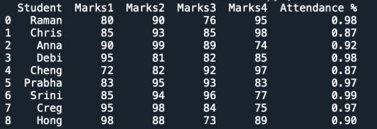
What is The Median Function Used For in Pandas?
Within Python, the programming language, libraries can be used to extend the functionality of code. One popular library is Pandas, stylized as Pandas. This library allows data scientists to manipulate and transform data in a variety of ways, but certain functions can be used to filter and sort data as well.
The MEDIAN function in pandas is an example of a function that does just that. Using the MEDIAN function in pandas, you’re able to call out the median number in a series or dataframe. A dataframe is like a spreadsheet within Python that contains an X-axis and a Y-axis.
Data from this table can be difficult to sort by sight, particularly when working with a large volume of data. Sorting via the MEDIAN function helps data scientists quickly ascertain the median number from a large group of number data.
How Can the MEDIAN Function Be Used?
You can use the MEDIAN function for a variety of things. For instance, if you were concerned about anomalies in your data, you could use the MEDIAN function to establish the median. This result will be most likely to represent a consistent trend among all the number data in a series or dataframe. With the median established in a dataset, you can establish thresholds to more easily identify anomalies in the future.
You can also use the MEDIAN function to determine the median cost of things like homes. A Realtor could work with a data scientist to establish the median home price in a particular area when working with tabular data. Realtors often gather data from their own internal sales as well as figures reported to national associations and public information provided to local governments.
This data could be imported from Excel or another spreadsheet program. Traditionally, the Realtor would need to go through each line by hand to determine the median value within the data, but the MEDIAN function can return this value instantly. Armed with this information, the Realtor can more accurately represent properties and guide buyers and sellers to the right opportunities.
Read a similar article about Excel functions in Python here at this page.
0 notes
Text
First off, beautiful art and I Will Also Die On The Hill Of Boone Turning Into A Lobster When Forced To Function In Direct Sunshine On The Mojave
But also I learned some trivia about fabric color, thickness, and sun exposure and am going to think WAY too hard about Boone's burn pattern. It is not critique. It is an infodump inspired by the glorious work above.
Boone's default is a white shirt. Assuming its a single ply cotton weave, that affects an SP of five. SP is a ratio calc. An SP 5 potency means it'll take 5 min for the sun to do the damage it would usually do in 1 minute.
So if it takes about 15 min in a desert enviroment to shart reddening up and 20 to burn lightly, 30 moderate, 40 severe, then the skin beneath his shirt would be lighter than the burn but darker than any part that isn't seeing *direct* sun exposure, with the palest bits being the underarms and the area around his sunglasses. Since treated glass specifically blocks UV and dims one's vision to reduce eye strain, it also creates a sorta reverse panda pattern with light circles forming around the eyes and slightly *below* since the strongest sun exposure is when the sun is at its zenith and the 3ish hours after that.
Boone probably hates taking off his shades because he's got that tanline going on XD
Also that means YES, CLOTHED SKIN CAN STILL BURN! If we accept Boone Burns Fast and say he reaches severe sunburn red in like 20 min, then he's only got an hour 40 before his shoulders are toast, too.
The barret, assuming it is made of the traditional felted wool, is thicker and UV resistant ( hair and fur both serving a radiation protection purpose across known life ) would affect a higher SP. However I do not know enough to calc an estimate time before burning.
Also if his shoulders are burnt his arms be blistering man this is why desert cultures opt for long and breezy in layers. Keeps irritants away and provides all over sun protection
Get this man some freakin sunblock Boone This Is How People Die Of Skin Cancer

sunburnt big boob big belly boone truthers unite
1K notes
·
View notes
Text
The Foundation of Clean Data Analysis
Clean data is the cornerstone of accurate and reliable data analysis. A robust foundation in data cleaning ensures that your insights are valid, consistent, and actionable. Here’s an outline of the foundational steps for clean data analysis:
1. Understanding the Dataset
Familiarize Yourself with the Data Understand the context of the dataset, including its purpose, variables, and expected outcomes. Tools: Data dictionaries, documentation, or domain expertise.
Inspect the Data Use methods like .head(), .info(), and .describe() in Python to gain an overview of the dataset's structure and summary statistics.
2. Identifying and Handling Missing Data
Locate Missing Data Identify missing values using functions like .isnull().sum() in Python. Visualization: Heatmaps (e.g., Seaborn) can highlight missing data patterns.
Strategies to Handle Missing Data
Removal: Drop rows or columns with excessive missing values.
Imputation: Fill missing values using statistical methods (mean, median, mode) or predictive models.
3. Addressing Outliers
Detect Outliers Use visualizations like boxplots or statistical methods like Z-scores and IQR to identify outliers.
Handle Outliers Options include capping, transformation, or removal, depending on the context of the analysis.
4. Resolving Inconsistencies
Standardize Data Formats Ensure consistency in formats (e.g., date formats, text capitalization, units of measurement). Example: Converting all text to lowercase using .str.lower() in Python.
Validate Entries Check for and correct invalid entries like negative ages or typos in categorical data.
5. Dealing with Duplicates
Detect Duplicates Use methods like .duplicated() to identify duplicate rows.
Handle Duplicates Drop duplicates unless they are meaningful for the analysis.
6. Ensuring Correct Data Types
Verify Data Types Check that variables have appropriate types (e.g., integers for counts, strings for categories).
Convert Data Types Use type-casting functions like astype() in Python to fix mismatched data types.
7. Data Transformation
Feature Scaling Apply normalization or standardization for numerical features used in machine learning. Techniques: Min-Max scaling or Z-score normalization.
Encoding Categorical Variables Use one-hot encoding or label encoding for categorical features.
Key Tools for Data Cleaning:
Libraries: Pandas, NumPy, Seaborn, Matplotlib (for Python users).
Software: Excel, OpenRefine, or specialized ETL tools like Talend or Alteryx.
By mastering these foundational steps, you’ll ensure your data is clean, consistent, and ready for exploration and analysis. Would you like more detailed guidance or code examples for any of these steps?
0 notes
Text
Lonsdor K518 PRO Fiat IMMO Update Car List & Add Key Guide
Lonsdor K518 PRO, K518 series have upgraded FIAT vehicle coverage for reading immo data & making dealer key on April 23, 2024. Read this article to learn how to update K518 Fiat immo software & program new keys.
Supported FIAT Car List: Grand Punto (2005-2014) 500 (2006-2017) Nemo (2007-2017) Bipper (2007-2017) Cinquecento (2007-2021) Mini Cargo (2008-2021) Qubo (2008-2021) Fiorino (2008-2021) New Fiorino (2008-2021) Punto (2009-2021) Punto Evo (2009-2021) Pratico (2010-2021) Doblo (2010-2021) Viaggio (2011-2018) Panda (2011-2021) 500C (2011-2021) Avventura (2014-2018) Egea (2018-2021) Tipo (2018-2021) Linea (2018-2021) 500X (2018-2021) 500E (2018-2021) New 500 (2020-2022) New 500C (2020-2022)

How to program Fiat's new key with K518 PRO? 1. Read Immo Data Immo & remote >> FIAT >> Select from vehicle >> Europe >> 500 >> Mechanical key >> 2006-2017 >> 70F3633_93C86_46 >> Read immo data Check the immo data, and press "OK". Save the immo data file. Reading successful. Can use this data to make the dealer key and then the program key. Note: if vehicle communication fails during subsequent function execution, please disconnect the vehicle battery for 1-2 mins and re-connect it, then retry the function.


2. Make Dealer Key Make dealer key >> OK >> Selected immo data file >> OK Push open the card slot's baffle on the device. Place the key to be generated into the K518 PRO card slot. Operating to the key, please wait... The dealer key was generated and locked successfully.


3. Add New Key Press the "Program key". This operation will delete all programmed keys, which need to be re-programmed before use, keys to be programmed need to be custom or dealer keys, press "OK" to continue. Please insert the key to be programmed, and switch the ignition ON. Enter PIN code. Programming succeed. Please switch the ignition off. Turn the ignition on. Current key count: 2 Programming complete.


www.obd2shop.co.uk
#lonsdor k518 pro#lonsdor k518 pro update#londsor k518#lonsdor k518 pro fiat#lonsdor k518#lonsdor k518 update
0 notes
Text
Battle of the Programming Languages: R vs Python

Battle of the Programming Languages: R vs Python
We are going to compare Functions exist in both R and Python for same operations. And for this we took the Titanic dataset which contains the Passenger details. Importing a CSV Reading Data in both the languages is similar, but the only difference is for python we have to import pandas library for reading the Data. Once the importing is done we can look into the data by applying the below functions.RPythontitanicimport pandas as pd
titanic = pd.read_csv("train.csv")
Dimension and Shape If we want to look the Dimension of the above imported Data. You can get it from the below functions.RPythondim(titanic)titanic.shape[1] 891 12(891, 12)
The above code brings you the number of passengers in titanic ship and the number of columns present in data. Head and Tail If you want to see some of the data like top rows (Any number of rows by default it gets 5 rows) or bottom rows form the Data frame. There are functions in similar functions in both R and Python.RPythonhead(titanic,2)titanic.head(2)PassengerId Survived Pclass
1 1 0 3
2 2 1 1
PassengerId Survived Pclass 0 1 0 3 1 2 1 1tail(titanic,2)titanic.tail(2) PassengerId Survived Pclass
890 890 1 1
891 891 0 3
PassengerId Survived Pclass 889 890 1 1
890 891 0 3
Here head and tail functions applied on Titanic dataset to look at the first two rows of Data. If you observe clearly the index values are different in both R and Python. It is because Python index starts with '0'. Basic Statistics of Data (Summary and Describe)RPythonsummary(titanic)titanic.describe()PassengerId SurvivedPassengerId SurvivedMin. : 1.0 Min. :0.0000
1st Qu.:223.5 1st Qu.:0.0000
Median :446.0 Median :0.0000
Mean :446.0 Mean :0.3838
3rd Qu.:668.5 3rd Qu.:1.0000
Max. : 891.0 Max. :1.0000count 891.000000 891.000000
mean 446.000000 0.383838
std 257.353842 0.486592
min 1.000000 0.000000
25% 223.500000 0.000000
50% 446.000000 0.000000
75% 668.500000 1.000000
max 891.000000 1.000000
The above two functions are for determining some basic statistics column wise. Whereas python gives two more statistic values compared to R function. The main difference between these functions is R contains Separate functions and for Python we have to call the required methods on the Data as it is more of object oriented type programming. Slicing the Datatitanic[1:5,1:3]titanic.iloc[0:5,0:3]PassengerId Survived Pclass
1 1 0 3
2 2 1 1
3 3 1 3
4 4 1 1
5 5 0 3PassengerId Survived Pclass
0 1 0 3
1 2 1 1
2 3 1 3
3 4 1 1
4 5 0 3
Sub setting Data Here in this case for sub setting the Data I took only some columns from the titanic Dataset. For the convenience of displaying the output. Using sam_data sam_data = titanic[['PassengerId', 'Survived','Sex','Age']] for Python I created sam_data for applying subset function. subset(sam_data,Survived == 1& Sex == 'male')sam_data[(sam_data.Sex == 'male') & (sam_data.Survived ==1)].head(2)PassengerId Survived Sex Age
18 18 1 male NA 22 22 1 male 34 24 24 1 male 28 37 37 1 male NA 56 56 1 male NA 66 66 1 male NAPassengerId Survived Sex Age
17 18 1 male NaN 21 22 1 male 34.00 23 24 1 male 28.00 36 37 1 male NaN 55 56 1 male NaN 65 66 1 male NaN
The important thing here is the representation of NA in Python is NaN. Ordering the Data We ordered the Sample Dataset By arrange(sam_data, Survived, desc(Age))sam_data.sort_index(by=['Survived', 'Age'], ascending=[True, False])PassengerId Survived Sex Age 1 852 0 male 74.0 2 97 0 male 71.0 3 494 0 male 71.0 4 117 0 male 70.5 5 673 0 male 70.0 6 746 0 male 70.0PassengerId Survived Sex Age 851 852 0 male 74.0 493 494 0 male 71.0 96 97 0 male 71.0 116 117 0 male 70.5 672 673 0 male 70.0 745 746 0 male 70.0
Joins For Performing join operations we created three different data frames from the titanic Dataset df_Survived df_Sex df_Age df_Survived = sam_data[['PassengerId', 'Survived']] df_Sex = sam_data [['PassengerId', 'Sex']] df_Age = sam_data [[ 'PassengerId', 'Age']] Inner
JoinTable_Inner_J = merge ( merge(df_Survived, df_Sex, key = "PassengerId" ),
df_Age ,
key = "PassengerId")Table_Inner_J = pd.merge ( pd.merge(df_Survived, df_Sex, on = "PassengerId" , how = "inner" ),
df_Age ,
on = "PassengerId" , how = "inner")Outer JoinTable_Outer_J = merge ( merge(df_Survived, df_Sex, key = "PassengerId" , all =TRUE),
df_Age ,
key = "PassengerId", all = TRUE)Table_Outer_J = pd.merge ( pd.merge(df_Survived, df_Sex, on = "PassengerId" , how = "outer"),
df_Age ,
on = "PassengerId", how = "outer")Left
JoinTable_Left_J = merge ( merge(df_Survived, df_Sex, key = "PassengerId" , all.x =TRUE),
df_Age ,
key = "PassengerId", all.x = TRUE)Table_Left_J = pd.merge ( pd.merge(df_Survived, df_Sex, on = "PassengerId" , how = "left"),
df_Age ,
on = "PassengerId" , how = "left")Right
JoinTable_Right_J = merge ( merge(df_Survived, df_Sex, key = "PassengerId", all.y = TRUE),
df_Age ,
key = "PassengerId", all.y = TRUE )Table_Right_J = pd.merge ( pd.merge(df_Survived, df_Sex, on = "PassengerId" , how = "right"),
df_Age ,
on = "PassengerId" , how = "right")
The major Difference in R and Python for joining operation is both can be done using merge function. But for python we have to import pandas library for using the merge function to perform these join functions. We can join three Data frames at a time by applying merge function two times. Missing Values Treatment: In Missing Values treatment first thing we have to do is identify the NA values by running the first block of code in below table. After getting the variables where missing values are there then you can impute them with the mean value of that respective column. Here, second block of code replaces the NA values with the respective mean values. tail(is.na(sam_data))sam_data.isnull().tail()PassengerId Survived Sex Age [886,] FALSE FALSE FALSE FALSE [887,] FALSE FALSE FALSE FALSE [888,] FALSE FALSE FALSE FALSE [889,] FALSE FALSE FALSE TRUE [890,] FALSE FALSE FALSE FALSE [891,] FALSE FALSE FALSE FALSEPassengerId Survived Sex Age 886 False False False False 887 False False False False 888 False False False False 889 False False False True 890 False False False Falsesam_data["Age"][is.na(sam_data["Age"])]meanAge = np.mean(sam_data.Age)
sam_data.Age = sam_data.Age.fillna(meanAge)PassengerId Survived Sex Age
[886,] FALSE FALSE FALSE FALSE
[887,] FALSE FALSE FALSE FALSE
[888,] FALSE FALSE FALSE FALSE
[889,] FALSE FALSE FALSE FALSE
[890,] FALSE FALSE FALSE FALSE
[891,] FALSE FALSE FALSE FALSEPassengerId Survived Sex Age
886 False False False False
887 False False False False
888 False False False False
889 False False False False
890 False False False False

About Rang Technologies: Headquartered in New Jersey, Rang Technologies has dedicated over a decade delivering innovative solutions and best talent to help businesses get the most out of the latest technologies in their digital transformation journey. Read More...
0 notes
Text
Demystifying Data Science: Essential Concepts for Beginners
In today's data-driven world, the field of data science stands out as a beacon of opportunity. With Python programming as its cornerstone, data science opens doors to insights, predictions, and solutions across countless industries. If you're a beginner looking to dive into this exciting realm, fear not! This article will serve as your guide, breaking down essential concepts in a straightforward manner.
1. Introduction to Data Science
Data science is the art of extracting meaningful insights and knowledge from data. It combines aspects of statistics, computer science, and domain expertise to analyze complex data sets.
2. Why Python?
Python has emerged as the go-to language for data science, and for good reasons. It boasts simplicity, readability, and a vast array of libraries tailored for data manipulation, analysis, and visualization.
3. Setting Up Your Python Environment
Before we dive into coding, let's ensure your Python environment is set up. You'll need to install Python and a few key libraries such as Pandas, NumPy, and Matplotlib. These libraries will be your companions throughout your data science journey.
4. Understanding Data Types
In Python, everything is an object with a type. Common data types include integers, floats (decimal numbers), strings (text), booleans (True/False), and more. Understanding these types is crucial for data manipulation.
5. Data Structures in Python
Python offers versatile data structures like lists, dictionaries, tuples, and sets. These structures allow you to organize and work with data efficiently. For instance, lists are sequences of elements, while dictionaries are key-value pairs.
6. Introduction to Pandas
Pandas is a powerhouse library for data manipulation. It introduces two main data structures: Series (1-dimensional labeled array) and DataFrame (2-dimensional labeled data structure). These structures make it easy to clean, transform, and analyze data.
7. Data Cleaning and Preprocessing
Before diving into analysis, you'll often need to clean messy data. This involves handling missing values, removing duplicates, and standardizing formats. Pandas provides functions like dropna(), fillna(), and replace() for these tasks.
8. Basic Data Analysis with Pandas
Now that your data is clean, let's analyze it! Pandas offers a plethora of functions for descriptive statistics, such as mean(), median(), min(), and max(). You can also group data using groupby() and create pivot tables for deeper insights.
9. Data Visualization with Matplotlib
They say a picture is worth a thousand words, and in data science, visualization is key. Matplotlib, a popular plotting library, allows you to create various charts, histograms, scatter plots, and more. Visualizing data helps in understanding trends and patterns.
Conclusion
Congratulations! You've embarked on your data science journey with Python as your trusty companion. This article has laid the groundwork, introducing you to essential concepts and tools. Remember, practice makes perfect. As you explore further, you'll uncover the vast possibilities data science offers—from predicting trends to making informed decisions. So, grab your Python interpreter and start exploring the world of data!
In the realm of data science, Python programming serves as the key to unlocking insights from vast amounts of information. This article aims to demystify the field, providing beginners with a solid foundation to begin their journey into the exciting world of data science.
0 notes
Text
A Beginner's Guide to Data Preprocessing in Machine Learning: Cleaning and Preparing Data for Analysis
Introduction:
Data is the fuel that powers the world of machine learning, but it's rarely in perfect shape when we first get our hands on it. Raw data is often messy, containing missing values, outliers, and inconsistencies that can negatively impact the performance of machine learning models. That's where data preprocessing comes in – a crucial step in the machine learning pipeline that involves cleaning and preparing the data to ensure it's in a suitable format for analysis. In this blog, we'll walk through the basics of data preprocessing and introduce some popular libraries to help you get started on your machine learning journey.
1. Importing the Necessary Libraries:
Before diving into data preprocessing, let's make sure we have the right tools at our disposal. We'll need to import the following libraries in Python:
- Pandas: For data manipulation and analysis.
- NumPy: For numerical operations and array processing.
- Matplotlib and Seaborn: For data visualization.
- Scikit-learn: For machine learning algorithms and additional preprocessing functions.
You can install these libraries using pip by running the following commands:
pip install pandas numpy matplotlib seaborn scikit-learn
2. Understanding the Data:
The first step in data preprocessing is to gain an understanding of the data you're working with. Look for the following aspects:
- The dimensions of the dataset (rows and columns).
- The types of features present (numerical, categorical, text, etc.).
- The presence of any missing values.
- Distribution of the target variable (for supervised learning tasks).
3. Handling Missing Data:
Missing data is a common issue in datasets and can lead to biased results if not handled properly. There are several approaches to deal with missing values:
- **Removal**: Remove rows or columns with missing values. However, this should be done with caution as it may result in a loss of valuable information.
- **Imputation**: Fill in missing values using various techniques such as mean, median, mode, or advanced imputation methods like K-nearest neighbors.
We can use Pandas to perform these operations:
import pandas as pd
# Load the dataset
data = pd.read_csv('your_dataset.csv')
# Check for missing values
print(data.isnull().sum())
# Impute missing values with mean
data.fillna(data.mean(), inplace=True)
4. Handling Categorical Data:
Machine learning models typically work with numerical data, so we need to convert categorical data into numerical form. One common technique is one-hot encoding, where each category becomes a binary column.
# One-hot encoding using pandas
data = pd.get_dummies(data, columns=['categorical_column'])
5. Feature Scaling:
Feature scaling ensures that all numerical features are on a similar scale, preventing certain features from dominating others during model training. Two popular scaling techniques are Min-Max scaling and Standardization.
from sklearn.preprocessing import MinMaxScaler, StandardScaler
# Min-Max Scaling
scaler = MinMaxScaler()
data[['feature1', 'feature2']] = scaler.fit_transform(data[['feature1', 'feature2']])
# Standardization
scaler = StandardScaler()
data[['feature1', 'feature2']] = scaler.fit_transform(data[['feature1', 'feature2']])
6. Handling Outliers:
Outliers can significantly impact model performance. You can visualize them using box plots and handle them using various techniques like truncation or capping.
import seaborn as sns
# Box plot to identify outliers
sns.boxplot(data=data[['feature1', 'feature2']])
7. Splitting the Data:
Before training the model, we need to split the data into training and testing sets. This allows us to evaluate the model's performance on unseen data.
from sklearn.model_selection import train_test_split
X = data.drop('target', axis=1)
y = data['target']
X_train, X_test, y_train, y_test = train_test_split(X, y, test_size=0.2, random_state=42)
Conclusion:
Data preprocessing is a critical step in the machine learning workflow, as it ensures that the data is cleaned and transformed into a suitable format for model training. In this blog, we covered the basics of data preprocessing, including handling missing data, categorical data, feature scaling, and outliers. By using libraries like Pandas, NumPy, Matplotlib, Seaborn, and Scikit-learn, you can effectively preprocess your data and set the foundation for building powerful machine learning models.
Remember that data preprocessing is not a one-size-fits-all process. Different datasets may require different preprocessing techniques, so always be prepared to explore and adapt your approach accordingly. Happy learning and good luck on your machine learning journey!
@TalentServe
#DataPreprocessing #MachineLearning #Cleaning #Analysis
0 notes
Text
min yoongi, the snowman

summary: yoongi does not care for the snowman (idol au, fluff)
pairing: min yoongi x reader
rating: PG-13
warnings: one swearword
words: 900
part of: Christmas with BTS | [masterlist]
“where is she?”, you can hear the frustration in min yoongi’s voice coming from the office right next to yours.
“i- i’m not, not entirely sure if sh-she’s in today.” kudos to your coworker for trying to lie. but you’re known for your non-existent social life – so where else would you be on the 25th of december?
you hear the famous idol huff before there is an uncomfortable silence. the woman across from your workspace breaks down faster than you thought.
“she’s… uhm she’s in room 204M.”
a few seconds later you can hear an unforgiving knock on your door. the idol walks into your space before you even answer him. he looks relaxed, wearing some stretch trousers and one of his iconic FG embroidered t-shirt. the sling around his neck reminds you of his recent operation and how glad you are to see him this agile not long after.
“min yoongi – to what do i owe this pleasant visit?” you try to act as dumb as possible – not a crass feat with how little sleep and how much caffeine your body has to work with.
the rapper looks around your desk in mocked disgust.
“you know how much sodium is in these?”, he says and points to the empty take-out boxes across your work surface. rude.
“just because you can’t eat panda express on your diet doesn’t mean you have to be mean”, you huff as you gather the empty containers to dispose them asap – it’s not the most professional environment to work in, you give him that.
yoongi moves to sit in the only other chair, facing you while you’re cleaning up the mess.
“_____”, he says with a hint of seriousness in his tone when you’re not giving him the needed attention. still your eyes dance across his face – the chubby cheeks, his darkish black locks, the lips shining from balm – not meeting his stare.
the man scoffs in annoyance and you take a deep breath before making eye contact.
“a snowman?”, yoongi asks and you can’t hold in the laughter at his betrayed expression.
“he even had my mic, ____”, he whines, and you stretch your back, still chuckling softly at the idol.
“to… to be fair, it was seokjin’s idea”, you answer his unspoken accusation, but the idol still glares at you – the production assistant.
“it was silly”, he argues, not ready to talk about all the ways he’ll make his hyung pay for that.
“it was cute.” their performance has been a hit; your feed is still overflown with gifs from their stages. you’ve done a really good job. however, the injured rapper is not happy with the prop for their last gayo in his hometown.
behind his childish attitude you see a young man who’s truly upset about not being with his coworkers, for not being on stage. and you get that – so you move closer, dragging your chair with you to sit next to him.
“min”, you start with a calming voice. “we did a lot these last weeks – we had jimin rapping your part, your art in the background – heck we even had your hologram a freaking CGI version of yourself there.” yoongi relaxes during your listing – still there’s sadness in his eyes. and you don’t like that, at all.
“it’s christmas, you know? that’s all holiday spirit and fanservice”, you reassure him and pat his healthy shoulder.
yoongi nods and watches your hands on him, not being able to look into your eyes directly.
“you’ll be on stage again soon enough.” your support – for the last three years, but especially during the last weeks – means a lot to him. there is a soft smile shying on his lips and you feel your own mouth stretch happily.
“why don’t i buy you some dumplings, hm? let’s eat!”, you exclaim and remove your hand from his warmth only to clap in excitement. “it’ll cheer you up, min!”, you add when you see how unsure he’s looking at you.
after a second of silent thoughts he nods reluctantly. “the fried ones?”, yoongi asks shyly as you move around your office to locate your wallet and cellphone.
you know he’s not supposed to eat oily stuff – you’ve glanced over their individual meal plans during the last meeting. nevertheless, the silent plea in his eyes is enough to soften your discipline.
“sure”, you answer, mentally adding lot of steamed vegetables to your order. “come on, min.”
obediently he gets up from his chair and helps you – rather clumsy with only one functioning hand – into your jacket.
while you shut off the lights and lock the door, you see him on his phone scrolling through weverse.
“it’s all full of this snowman, ____”, he whines, which makes you coo at his childlike tantrum.
“he’s cute, though, you can’t deny that”, you argue only to receive a death glare.
“yeah – sure, because i’m the member responsible for all the cuteness in this group, right”, he mutters and presses the elevator button with a bit too much force.
“what’s next? you’ll just put a cat in front of a mic for the tbs awards?”, yoongi jokes and throws his healthy arm over your shoulder as the elevator doors close to give you some privacy.
“the internet would break”, you snort and join his throaty chuckle.
later that night seokjin’s inbox lights up with a new message from his favorite production assistant, long term friend and partner in crime:
____
re: re: re: re: lil meow meow tbs awards
MISSION ABORT
writing this made me really soft, i hope reading is just as much fun! if they have a kitten present during their performance on the 30th, i want compensations!
have a lovely day! love, dana
#yoongi x reader#yoongi x you#yoongi fluff#yoongi drabble#bts christmas fanfic#bts x reader#bts x you#idol au#yoongi fanfic#min yoongi
169 notes
·
View notes
Note
Bitch you and panda better sleep @thesexypanda-boo
ha hOW
I have to leave for the wedding function in 20 mins and I slept for like 45 mins in the afternoon if it matters
oh and btw I'm not gonna be back around like 1 am so fuck me
12 notes
·
View notes
Text
Week - 1 Assignment, Analysis Of Variance
clear all
""" Week - 1 Assignment, Analysis Of Variance
Hypothesis - Do people tend to have more beer as they have more members above 18 years in the household to give them company
Variables chosen for this analysis
How often you consumer beer - S2AQ5B should be less than 99 (page 33 of NESARC) No of beers you drink - S2AQ5D should be less than 99 (page 33 of NESARC) No of persons 18 years and older in the household - NUMPER18 (page 2 of NESARC)
Null Hypothesis :The Average Number of Beers consumed is not different across families having 1 household member, 2 to 3 household members 4 to 6 household members and greater than 6 household members who are older than 18 years old
Alternate Hypothesis : The Average Number of Beers consumed is different across families having 1 household member, 2 to 3 household members 4 to 6 household members and greater than 6 household members who are older than 18 years old
If the Alternate Hypothesis is proved right, then does it mean that household members having greater than 6 members tend to consume more beer ?
@author: Keerthi Kumar ([email protected]) """
import numpy as np import pandas as pd import statsmodels.formula.api as smf import statsmodels.stats.multicomp as multi
data = pd.read_csv('E:\\My_Learnings\\Yorbit\\20200921_Data_Analysis_Tools\\week_1\\dataset\\nesarc.csv', low_memory=False)
#setting variables to numeric data['S2AQ5B'] = data['S2AQ5B'].convert_objects(convert_numeric=True) data['S2AQ5D'] = data['S2AQ5D'].convert_objects(convert_numeric=True) data['NUMPER18'] = data['NUMPER18'].convert_objects(convert_numeric=True)
#subset data for respondents who have consumed beer sub1=data[(data['S2AQ5B']<99) & (data['S2AQ5D']<=99)] len(sub1) #18291 Records
#subset data only for required columns sub2 = sub1[["S2AQ5B", "S2AQ5D","NUMPER18"]] len(sub2) #18291 Records
#checking for any missing records sum(pd.isnull(sub2['S2AQ5B'])) # No Records are null sum(pd.isnull(sub2['S2AQ5D'])) # No Records are null sum(pd.isnull(sub2['NUMPER18'])) # No Records are null
#converting the explanatory variable (i.e The number of members in a household - S2AQ5D) # converting the explanatory variable into 4 bins where # Bin 1 - 1 household member, Bin 2 - 2 to 3 household members, Bin 3 = 4 to 6 household members, Bin 34 = greater than 6 household members
#checking for levels in the data print(sub2['NUMPER18'].min()) print(sub2['NUMPER18'].max())
#creating bins in the data for the explanatory variable i.e Number18- Number of household members greater than 18 in the family sub2['Family_members_bin']=pd.cut(x = sub2['NUMPER18'], bins = [0,1,3,4,9], labels = [1,2,3,4]) sub2.head() check_bins = sub2.groupby('Family_members_bin').agg({'NUMPER18': ['min', 'max']}) print(check)
#checking for average number of beers consumed across groups and frequency within the groups stats_beer = sub2.groupby('Family_members_bin').agg({'S2AQ5D': ['mean','std','size']}) print(stats_beer) # Interpretation - It appears that the average consumption is different across groups but whether it is significant is the question
# using ols function for calculating the F-statistic and associated p value model1 = smf.ols(formula='S2AQ5D ~ C(Family_members_bin)', data=sub2) results1 = model1.fit() print (results1.summary())
mc1 = multi.MultiComparison(sub2['S2AQ5D'], sub2['Family_members_bin']) res1 = mc1.tukeyhsd() print(res1.summary())
""" Null Hypothesis - The average consumption of beer is not different between different size of Households for members of the households being older then 18 years Alternate Hypothesis - The average consumption of beer is different between different size of Housolds for members of the households being older than 18 years
A. Initial Analysis Interpretation
mean std size Family_members_bin 1 2.897834 6.043876 6509 2 2.729754 4.724074 11101 3 3.608611 6.703192 511 4 3.323529 3.206139 170 Label 1 - 1 household member older than than 18 years 2 - 2 to 3 household members older than 18 years 3 - 4 to 6 household members older than 18 years 4- greater than 6 household members older than 18 years
a. From the above analysis, it is evident that the means are different between the groups. b. It is very clear that group 3 and group 4 have higher consumption of beer c. However it is unclear if 1 and 2 are different from each other, also if 3 and 4 are different from each other
B. Results from the F - Test and OLS results
OLS Regression Results ============================================================================== Dep. Variable: S2AQ5D R-squared: 0.001 Model: OLS Adj. R-squared: 0.001 Method: Least Squares F-statistic: 5.864 Date: Tue, 22 Sep 2020 Prob (F-statistic): 0.000536 Time: 18:18:12 Log-Likelihood: -56392. No. Observations: 18291 AIC: 1.128e+05 Df Residuals: 18287 BIC: 1.128e+05 Df Model: 3 Covariance Type: nonrobust ============================================================================================== coef std err t P>|t| [0.025 0.975] ---------------------------------------------------------------------------------------------- Intercept 2.8978 0.065 44.267 0.000 2.770 3.026 C(Family_members_bin)[T.2] -0.1681 0.082 -2.039 0.042 -0.330 -0.006 C(Family_members_bin)[T.3] 0.7108 0.243 2.929 0.003 0.235 1.186 C(Family_members_bin)[T.4] 0.4257 0.410 1.037 0.300 -0.379 1.230 ============================================================================== Omnibus: 34676.204 Durbin-Watson: 2.005 Prob(Omnibus): 0.000 Jarque-Bera (JB): 53125932.316 Skew: 14.817 Prob(JB): 0.00 Kurtosis: 265.354 Cond. No. 12.6 ==============================================================================
Warnings: [1] Standard Errors assume that the covariance matrix of the errors is correctly specified.
Analysis Interpretation- The prob fstatistic is less than 0.05 and hence we could reject the null hypothesis and accept the alternate hypothesis stating that the groups have different consumption behavior.
C. Results from the Post Hoc multiple comparisons test
Multiple Comparison of Means - Tukey HSD,FWER=0.05 ============================================ group1 group2 meandiff lower upper reject -------------------------------------------- 1 2 -0.1681 -0.3799 0.0438 False 1 3 0.7108 0.0874 1.3342 True 1 4 0.4257 -0.6285 1.4799 False 2 3 0.8789 0.2649 1.4928 True 2 4 0.5938 -0.4549 1.6424 False 3 4 -0.2851 -1.4865 0.9164 False
Analysis Interpretation - a. Group 1 (1 household member older than 18 years) consume significantly less quantum of beer than than Group 3 (4 to 6 households members older than 18 years). b. Group 2 (2 to 3 household member older than 18 years) consume significantly less beer than than Group 3 (4 to 6 households members older than 18 years). c. However this relation does not seem to hold for the larger group when then there are more than 6 members in the household.
"""
2 notes
·
View notes
Text
Coursera Data Analysis Tools: Lesson
Model Interpretation for ANOVA:
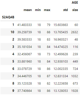
When examining the association between the AGE of the respondants of the nesarc_pds sample (quantitative response) and how often that person drank coolers in the last 12 months (categorical explanatory), an Analysis of Variance (ANOVA) revealed mean age difference among the groups of alcohol drinkers in a statistically significant association with an F(9, 7901)= 29.19, p << 0.00001 (1.59e-50). This concludes there is a relation between the age of drinkers and the amount of driking.
Model Interpretation for post hoc ANOVA results:
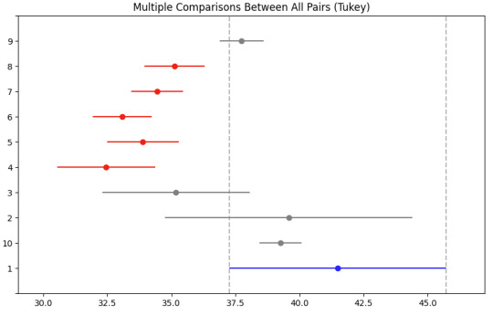
Post Hoc comparisons of mean age of drinkers between groups reported a significant different in age for heavy drinkers (group 1) and ocassionally drinkers (group 10) with those that frequently drink (groups 4, 5, 6, 7, 8)
Code:
Coursera Assignment
import pandas as pd import numpy as np import statsmodels.formula.api as smf import statsmodels.stats.multicomp as multi
df = pd.read_csv('nesarc_pds.csv')
#Restrict table to only 2 columns that we will work with:
anova_df = df[['S2AQ4B', 'AGE']].dropna()
Remove empty or NA values
anova_df['S2AQ4B'].replace({'99':np.NaN, 'BL':np.NaN, ' ':np.NaN}, inplace=True) anova_df.dropna(inplace=True)
#convert 'S2AQ4B' to int
anova_df['S2AQ4B'].astype('int64',copy=False)
#Get a sense of number of instances per type
anova_df.groupby('S2AQ4B').agg({'AGE': ['mean', 'min', 'max', 'std', 'size']})
#using ols function for calculating the F-statistic and associated p value
model1 = smf.ols(formula='AGE ~ C(S2AQ4B)', data=anova_df) results1 = model1.fit() results1.summary()
#Post Hoc Test between groups
mc1 = multi.MultiComparison(anova_df['AGE'], anova_df['S2AQ4B']) res1 = mc1.tukeyhsd() res1.summary()
1 note
·
View note
Text
Calculate Summary Statistics in Pandas
Calculate Summary Statistics in Pandas
How to perform Pandas summary statistics on DataFrame and Series? Pandas provide the describe() function to calculate the descriptive summary statistics. By default, this describe() function calculates count, mean, std, min, different percentiles, and max on all numeric features or columns of the DataFrame. Table of contents1. Summary Statistics Functions2. Pandas describe() Syntax & Usage2.1…
View On WordPress
0 notes
Text
Assignment 4 - Data Visualization
import pandas import numpy import seaborn import matplotlib.pyplot as plt
data = pandas.read_csv('gapminder.csv', low_memory=False)
data = data.replace(r'^\s*$', numpy.NaN, regex=True)
#setting variables you will be working with to numeric
data['internetuserate'] = pandas.to_numeric(data['internetuserate']) data['urbanrate'] = pandas.to_numeric(data['urbanrate']) data['incomeperperson'] = pandas.to_numeric(data['incomeperperson']) data['hivrate'] = pandas.to_numeric(data['hivrate'])
desc1 = data['urbanrate'].describe()
#The below are descriptive statistics results for all the 2 variables used in the code
print (desc1)
count 203.000000
mean 56.769360
std 23.844933
min 10.400000
25% 36.830000
50% 57.940000
75% 74.210000
max 100.000000
desc2 = data['internetuserate'].describe() print (desc2)
count 192.000000
mean 35.632716
std 27.780285
min 0.210066
25% 9.999604
50% 31.810121
75% 56.416046
max 95.638113
#basic scatterplot: Q->Q
scat1 = seaborn.regplot(x="urbanrate", y="internetuserate", fit_reg=False, data=data)
plt.xlabel('Urban Rate')
Text(0.5, 0, 'Urban Rate')
plt.ylabel('Internet Use Rate')
Text(0, 0.5, 'Internet Use Rate')
plt.title('Scatterplot for the Association Between Urban Rate and Internet Use Rate')
Text(0.5, 1.0, 'Scatterplot for the Association Between Urban Rate and Internet Use Rate')
scat2 = seaborn.regplot(x="urbanrate", y="internetuserate", data=data)
#scatterplot graph image cannot be attached here
plt.xlabel('Urban Rate')
Text(0.5, 0, 'Urban Rate')
plt.ylabel('Internet Use Rate')
Text(0, 0.5, 'Internet Use Rate')
plt.title('Scatterplot for the Association Between Urban Rate and Internet Use Rate')
Text(0.5, 1.0, 'Scatterplot for the Association Between Urban Rate and Internet Use Rate')
scat3 = seaborn.regplot(x="incomeperperson", y="internetuserate", data=data)
#scatterplot graph image cannot be attached here
plt.xlabel('Income per Person')
plt.ylabel('Internet Use Rate')
plt.title('Scatterplot for the Association Between Income per Person and Internet Use Rate')
scat4 = seaborn.regplot(x="incomeperperson", y="hivrate", data=data)
plt.xlabel('Income per Person')
plt.ylabel('HIV Rate')
plt.title('Scatterplot for the Association Between Income per Person and HIV Rate')
#quartile split (use qcut function & ask for 4 groups - gives you quartile split)
print ('Income per person - 4 categories - quartiles')
data['INCOMEGRP4']=pandas.qcut(data.incomeperperson, 4, labels=["1=25th%tile","2=50%tile","3=75%tile","4=100%tile"])
c10 = data['INCOMEGRP4'].value_counts(sort=False, dropna=True)
print(c10)
1=25th%tile 48
2=50%tile 47
3=75%tile 47
4=100%tile 48
#bivariate bar graph C->Q
seaborn.catplot(x='INCOMEGRP4', y='hivrate', data=data, kind="bar", ci=None)
#bar chart image cannot be attached here
plt.xlabel('income group')
plt.ylabel('mean HIV rate')
c11= data.groupby('INCOMEGRP4').size()
print (c11)
INCOMEGRP4
1=25th%tile 48
2=50%tile 47
3=75%tile 47
4=100%tile 48
#Summary:
We examined four variables - internateuser rate, urban rate, income per person and HIV rate from gapminder dataset and understand each variables descriptive statistics.
Next we did a co-relation analysis on these variables to find association b/w them. From the urban rate & internet use rate we find there is positive relation b/w them.
plt.xlabel('Urban Rate')
plt.ylabel('Internet Use Rate')
plt.title('Scatterplot for the Association Between Urban Rate and Internet Use Rate')
scat3 = seaborn.regplot(x="incomeperperson", y="internetuserate", data=data)
plt.xlabel('Income per Person')
plt.ylabel('Internet Use Rate')
plt.title('Scatterplot for the Association Between Income per Person and Internet Use Rate')
Text(0.5, 1.0, 'Scatterplot for the Association Between Income per Person and Internet Use Rate')
scat4 = seaborn.regplot(x="incomeperperson", y="hivrate", data=data)
plt.ylabel('HIV Rate')
plt.title('Scatterplot for the Association Between Income per Person and HIV Rate')
0 notes
Text
Assignment 3
Output with Frequency Tables at High Suicide Rate for Breast Cancer Rate, HIV Rate and Employment Rate Variables
Statistics for a Suicide Rate count 191.000000 mean 9.640839 std 6.300178 min 0.201449 25% 4.988449 50% 8.262893 75% 12.328551 max 35.752872
Number of Breast Cancer Cases with a High Suicide Rate
of Cases Freq. Percent Cum. Freq. Cum. Percent
(1, 23] 18 33.96 18 33.96 (23, 46] 15 28.30 33 62.26 (46, 69] 10 18.87 43 81.13 (69, 92] 8 15.09 51 96.23 nan 2 3.77 53 100.00
HIV Rate with a High Suicide Rate Rate Freq. Percent Cum. Freq. Cum. Percent 0% tile 18 33.96 18 33.96 25% tile 8 15.09 26 49.06 50% tile 11 20.75 37 69.81 75% tile 12 22.64 49 92.45 nan 4 7.55 53 100.00
Employment Rate with a High Suicide Rate Rate Freq. Percent Cum. Freq. Cum. Percent 1 10 18.87 10 18.87 2 24 45.28 34 64.15 3 5 9.43 39 73.58 4 13 24.53 52 98.11 5 1 1.89 53 100.00
Summary of Frequency Distributions
I grouped the breast cancer rate, HIV rate and employment rate variables to create three new variables: bcgroup4, hcgroup4 and ecgroup4 using three different methods in Python. The grouped data also includes the count for missing data.
1) For the breast cancer rate, I grouped the data into 4 groups by number of breast cancer cases (1-23, 24-46, 47-69, 70-92) using pandas.cut function. People with lower breast cancer rate experience a high suicide rate. 2) For the HIV rate, I grouped the data into 4 groups by quartile pandas.qcut function. People with lower HIV rate experience a high suicide rate. 3) For the employment rate, I grouped the data into 5 categorical groups using def and apply functions: (1:32-50, 2:51-58, 3:59-64, 4:65-83, 5:NAN). The employment rate is between 51%-58% for people with a high suicide rate.
Python Program
import pandas as pd
load gapminder dataset
data = pd.read_csv('gapminder.csv',low_memory=False)
lower-case all DataFrame column names
data.columns = map(str.lower, data.columns)
bug fix for display formats to avoid run time errors
pd.set_option('display.float_format', lambda x:'%f'%x)
setting variables to be numeric
data['suicideper100th'] = data['suicideper100th'].convert_objects(convert_numeric=True) data['breastcancerper100th'] = data['breastcancerper100th'].convert_objects(convert_numeric=True) data['hivrate'] = data['hivrate'].convert_objects(convert_numeric=True) data['employrate'] = data['employrate'].convert_objects(convert_numeric=True)
display summary statistics about the data
print("Statistics for a Suicide Rate") print(data['suicideper100th'].describe())
subset data for a high suicide rate based on summary statistics
sub = data[(data['suicideper100th']>12)]
make a copy of my new subsetted data
sub_copy = sub.copy()
BREAST CANCER RATE
frequency and percentage distritions for a number of breast cancer cases with a high suicide rate
include the count of missing data and group the variables in 4 groups by number of
breast cancer cases (1-23, 24-46, 47-69, 70-92)
bc_max=sub_copy['breastcancerper100th'].max() # maximum of breast cancer cases
group the data in 4 groups by number of breast cancer cases and record it into new variable bcgroup4
sub_copy['bcgroup4']=pd.cut(sub_copy.breastcancerper100th,[0bc_max,0.25bc_max,0.5bc_max,0.75bc_max,1*bc_max])
frequency for 4 groups of breast cancer cases with a high suicide rate
bc=sub_copy['bcgroup4'].value_counts(sort=False,dropna=False)
percentage for 4 groups of breast cancer cases with a high suicide rate
pbc=sub_copy['bcgroup4'].value_counts(sort=False,dropna=False,normalize=True)*100
cumulative frequency and cumulative percentage for 4 groups of breast cancer cases with a high suicide rate
bc1=[] # Cumulative Frequency pbc1=[] # Cumulative Percentage cf=0 cp=0 for freq in bc: cf=cf+freq bc1.append(cf) pf=cf*100/len(sub_copy) pbc1.append(pf)
print('Number of Breast Cancer Cases with a High Suicide Rate') fmt1 = '%10s %9s %9s %12s %13s' fmt2 = '%9s %9.d %10.2f %9.d %13.2f' print(fmt1 % ('# of Cases','Freq.','Percent','Cum. Freq.','Cum. Percent')) for i, (key, var1, var2, var3, var4) in enumerate(zip(bc.keys(),bc,pbc,bc1,pbc1)): print(fmt2 % (key, var1, var2, var3, var4))
HIV RATE
frequency and percentage distritions for HIV rate with a high suicide rate
include the count of missing data and group the variables in 4 groups by quartile function
group the data in 4 groups and record it into new variable hcgroup4
sub_copy['hcgroup4']=pd.qcut(sub_copy.hivrate,4,labels=["0% tile","25% tile","50% tile","75% tile"])
frequency for 4 groups of HIV rate with a high suicide rate
hc = sub_copy['hcgroup4'].value_counts(sort=False,dropna=False)
percentage for 4 groups of HIV rate with a high suicide rate
phc = sub_copy['hcgroup4'].value_counts(sort=False,dropna=False,normalize=True)*100
cumulative frequency and cumulative percentage for 4 groups of HIV rate with a high suicide rate
hc1=[] # Cumulative Frequency phc1=[] # Cumulative Percentage cf=0 cp=0 for freq in hc: cf=cf+freq hc1.append(cf) pf=cf*100/len(sub_copy) phc1.append(pf)
print('HIV Rate with a High Suicide Rate') print(fmt1 % ('Rate','Freq.','Percent','Cum. Freq.','Cum. Percent')) for i, (key, var1, var2, var3, var4) in enumerate(zip(hc.keys(),hc,phc,hc1,phc1)): print(fmt2 % (key, var1, var2, var3, var4))
EMPLOYMENT RATE
frequency and percentage distritions for employment rate with a high suicide rate
include the count of missing data and group the variables in 5 groups by
group the data in 5 groups and record it into new variable ecgroup4
def ecgroup4 (row): if row['employrate'] >= 32 and row['employrate'] < 51: return 1 elif row['employrate'] >= 51 and row['employrate'] < 59: return 2 elif row['employrate'] >= 59 and row['employrate'] < 65: return 3 elif row['employrate'] >= 65 and row['employrate'] < 84: return 4 else: return 5 # record for NAN values
sub_copy['ecgroup4'] = sub_copy.apply(lambda row: ecgroup4 (row), axis=1)
frequency for 5 groups of employment rate with a high suicide rate
ec = sub_copy['ecgroup4'].value_counts(sort=False,dropna=False)
percentage for 5 groups of employment rate with a high suicide rate
pec = sub_copy['ecgroup4'].value_counts(sort=False,dropna=False,normalize=True)*100
cumulative frequency and cumulative percentage for 5 groups of employment rate with a high suicide rate
ec1=[] # Cumulative Frequency pec1=[] # Cumulative Percentage cf=0 cp=0 for freq in ec: cf=cf+freq ec1.append(cf) pf=cf*100/len(sub_copy) pec1.append(pf)
print('Employment Rate with a High Suicide Rate') print(fmt1 % ('Rate','Freq.','Percent','Cum. Freq.','Cum. Percent')) for i, (key, var1, var2, var3, var4) in enumerate(zip(ec.keys(),ec,pec,ec1,pec1)): print(fmt2 % (key, var1, var2, var3, var4))
0 notes
Text
How Should I Start Learning Python Programming for AI
This is a great question on two folds. Firstly, you are interested in learning a programming language, in this case Python, which indicates that you are interested in stepping into the world of IT. The basic requirement to start your career in IT is to learn a programming language. It is like learning your mother tongue, without which you cannot learn any other language such as English, French or Hindi. Secondly, you showing interest in Python indicates that you are inclined towards world of Data Science or AI. Of course, Python could be used for web or software development however, going by current trend Python is widely associated with those interested in the world of DS or AI.
What is Python

As we established the premise that learning Python is a basic requirement to step into the IT world and especially into DS or AI domains let’s focus on the part of how to learn. Python is a high level, general purpose language. High-level because you would code in a human understandable language (print, input, max, min,…) and General because you could use to build games, applications, machine learning, etc. Python is a open source interpreted language that is supported by community to help you learn better. It is as powerful as any other popular programming language yet simpler in structure. If you look at the TIOBE ratings, Python ranked 3 among all the popular programming languages. To top it top, if you look at the last column the change of rating is positive whereas for others it is negative. This indicates that Python is getting more and more audience. Hence, it is right decision to learn Python.
Why to Learn Python Focusing on the learning part, Python is simple to learn. Period.��It is a syntax friendly, object oriented, strongly typed, no frills programming language. I have worked on various languages but when I started exploring Python is fell in love with it. Even though it has it’s limitations, overall it is a good programming language to start your journey. Let me disclose one more fact. In the field of IT if you learn one Object Oriented Programming Language you could learn or catch up with any other programming language. This is primarily due to the common underlying principles, structure, methods, etc. Do you think that every time a new language or framework pops up all the IT guys would go back to classrooms to learn? No, they just use their existing know how to self-learn the new one. Hence, if you learn Python you could easily learn other languages too.
Python is Easy to Learn Saying that Python is easy to learn and hard to master. It is simple and syntax friendly however as you dive deeper it can challenge you. Hence, it is safe to say your diving should depend on what you want to achieve from learning Python. In case you are interested in Machine Learning then learning Python basics, conditional Statements, loops, bit of functions, etc. would suffice and you would move on with Python libraries i.e. NumPy and Pandas and eventually ML algorithms. However, in case you are interested in development side of the business that you would go deeper towards advanced, functions, Oops, error handling, Reg Exp., Modules & Packages, Date & Time. Git & GitHub, etc. This is how structured our Python Course and machine learning course curriculum to meet the needs of the students rather than teaching everything to everyone. Try to figure out goal, i.e. Learning based systems or Logic based systems which would clear how much you should learn.

How to Schedule & Learn Python? By now you must be clear on What is Python, Purpose & Goal, etc. Let’s focus on HOW part of it. To learn python start with scheduling. If you could schedule 2 hours per day of dedicated time for Python. You could learn it in 20 days. Yes, don’t be surprised. As I have mentioned it is easy to learn and hard to master. You could achieve beginner level with 30 - 50 hours of practice. Then you could decide whether to get along with other dependent paths like machine learning or dive deep into the advanced concepts. Bottom line there is ‘No Alternative to Practice’. Difference between a good Python programmer and the normal one is number of hours of investment. Gone are the days where information was limited. Currently, you have various sources (text, audio, video, etc.) offering variety and volume of learning material. You could find a source that suits your learning style and carry on with your learning. Write down a target date of 20 days from your start date and go for it.
Why it is becoming hard to Learn? You may wonder why does students fail to learn in spite of having so much online support and free courses. The answer is structured program and hand holding. Most of us are tuned to the teacher centric learning where we expect the teacher to guide us through the learning by offering a structure program and solve queries however silly they are. The online video based program fail to fill the gaps in the knowledge student might have developed during learning which would multiply over the time and eventually students gets disengaged from the learning path. Also these online programs are marketing activities to attract students to their platforms or courses.
Hence, they would not cover the essentials and the way you prefer to learn. Even we had this challenge at SchoolforAI while catering to students from India and Western world. We could solve it using Hybrid learning. You could follow SchoolforAI course curriculum in case you need help with planning
Opportunities There are every growing demand for Python developers, Data Analysts, Data Scientist, and so on. For all these Python is the baseline. As more and more organizations are leaning towards using Python at the core of their applications the demand for Python professionals is increasing. The salaries for these professionals are ranging anywhere from 10L per annum to 20L per annum depending on their expertise and independent working capabilities. Even the freshers are drawing hefty packages without much difficulty.
Conclusion As a conclusion you take my word on the face value that Python is a great programming language and easy to learn. Just start with installing the Python IDLE and Jupiter notebook (Anaconda Distribution). You don’t need anything more than that. In Parallel work on your soft skills too as you may be good at programming but there is an interview to clear. I have personally witnessed best of the students could not get through interview due to lack of soft skills rather than technical skills. Most of the good organization recruit candidates not just for today but for tomorrow. Good luck and hopefully we would meet again soon.
#python#python course#pythonlanguage#aicourse#ai#ai training institute#best artificial intelligence course#artificial intelligence#technology#coding#pythonprogramming#python programming for ai
1 note
·
View note
Text
PLEASE SIGNAL BOOST: I need to raise money for myself and a friend, both currently homeless.
THE SHORT VERSION:
-I am in India without access to my money due to a pickpocketing and bank-related technicalities.
-I am without housing due to repeated, egregious, explicit discrimination. This has depleted most of my funds and I relocated to Calcutta due to air quality, low cost of living, and beef.
-At the same time, a close friend and her partner (located in Delhi and Paris, respectively) have brought to my attention a friend of theirs who is literally being physically restrained in an abusive marriage. We are talking black eyes and bruises. It's a horrific situation but I need her also because she speaks Bengali. So the house hunting process is stalled until she escapes.
-I am staying at an airbnb very close to her place. Even after we manage to get her physically removed there'a more stuff we have to do like filing a police report etc. The airbnb is expensive by Calcutta standards, but it's cheaper than rent anywhere I've lived in the USA.
-I need money for two reasons: to pay the deposit on our flat, and to keep me alive until I can sort things out with the bank, which may not be possible until after I move into a permanent place.
THE SHORTER VERSION:
-Idiot foreigner and victim of ongoing battering need rescue funds so we don't die.
PLEASE SIGNAL BOOST THIS
Paypal here.
https://www.paypal.me/pcoolpearl
Further details under cut.
ON THE PICKPOCKETING AND BANK ISSUES:
-I was pickpocketed in the market about two months ago. That's life. It happens. Welcome to India. Some idiot got like 200 rupees so that's great for them but I had to cancel all my bank cards. Not really much I could do. I just got home and realised my wallet wasn't there anymore.
-Delhi does not have a functional mailing system at all. This means that the banks were more or less at a loss for how to get the cards at me. This is part of why I relocated to Calcutta. That's Bank Account A. The easy one, but also the far smaller one.
-But as for the larger and more consequential Bank Account B, which contains easily enough money for me to live off of in Calcutta for quite some time, they do not have any kind of policy for what to do in the event that someone ever manages to escape the land of the free and the home of the brave. This is the one tied to my social security payments, and is where all my money lives.
-So when I called Social Security they did that thing they do where they try to play gotcha with inconsistencies in your story. In my case I had already tried to get a replacement card weeks earlier, for reasons unrelated. "If it didn't get there weeks ago, wouldn't you have called weeks ago?" "What the fuck? No, I didn't solve any of the problems so why would I have called again and wasted my fucking time on this fucking phone line for no reason, again?" This was after a good 15 mins or so of this kind of grilling, which I find especially grating now after almost a year of living in countries where nobody can lie for shit and so there'a no point in every single fucking person pretending they're a TV detective whose purpose in life is to stop Moriarty from abusing welfare benefits. "If you're going to raise your voice at me, what I'm going to do is I'm going to place a security hold on your account and you'll need to verify your identity." Let me reiterate that she stated explicitly that this was in retaliation for raising my voice and not due to any real suspicion about my identity. In later calls to Social Security it would be revealed that she could
have easily seen on her computer that the card never got to me. That is information very easily verifiable by the World's Greatest Goddamn Detective over there.
-So the next person I called sent me on a wild goose chase to the American Embassy to pick up a form called a Memorandum of Understanding. Judging that the very limited funds I'd had stockpiled in my dresser was not best spent on an auto ride, I walked nearly an hour from the metro station to the embassy. There was a dust storm in this period and I read later that over a hundred people fucking died in it, but I just kept walking towards it because that's where the embassy was. Also I'd never seen a dust storm in my life and had no idea what it was or why the sky was pink.
-When I got there they told me straight up that 1. they don't do mail pickup, which is why the card hadn't gotten to me, and 2. they don't do memorandums of understanding. They offered to send me a different form for 50 USD. "Can't you borrow it?" they asked. "That's not a reasonable thing to say to someone who lives in India," I said straight up. "That's not a real amount of money that people in India have." That's American for "fuck off". So they wrote me a different letter in an attempt to verify my identity. I send this in with my only other forms of identification: my passport and an expired driver's license from Washington state. Waited 3 business days as instructed.
-They told me they can't use these because of issues relating to my legal name change a couple years ago. Social Security had not been updated as regards the change. "I have my birth certificate and my court certification for the name change, and I can fax those in."
-"What you'll have to do is go to you social security office in person--" "Look, I'm gonna cut you off there. You can see my current address right? Read that off to me. What city is that in." "New Delhi." "That's right, New Delhi. What country is that in? Great. So can, can you tell me where my local Social Security office is here in India?" She could not tell me where my local social security office was in India. There aren't any. That's why she couldn't tell me that. But again, no protocol for this situation and if an American bureaucrat breaks their protocol I'm 90% sure Obama's legally allowed to kill them.
-What I'll need to do is a complicated process involving appointing Americans to act as proxies to go in and file paperwork on my behalf. There are other ideas, but none of them are more sure or less complicated, and they all require me to have a permanent address.
ON WHY I DO NOT HAVE A PERMANENT ADDRESS:
-Those close to me know that I have had a hell of a time finding housing in India. It's not all that bad for an Indian to find housing and when my Indian friends have tried they've consistently been able to find me something in a few hours. But that something is living alone. Which 1. is depressing and 2. is tactically disadvantageous when you don't speak the language of a country because how you will tell the food panda guy where to go...
-So I moved in with an Indian girl who seemed nice enough, and her sister who seemed if anything even nicer. This was about a week before I was pickpocketed as described above.
-In India there's this big thing about vegetarianism where it's a highly important in determining one's role in caste hierarchy. Unfortunately for me I do not give a shit and think the caste system is dumb and scrambled myself some eggs. The disgust my caste Hindu roommates displayed towards me from that point on was palpable. Within another week they were asking me to leave. They got the landlord on their side fairly easily because that's how the caste system works and I was given less than a week to vacate. (To my knowledge there is no law like in USA saying they can't do that.) (Also if you're going to try to argue with me about how caste works shut up, I don't care, not the time.)
-The next day I would eat a straight-up poisoned "cheeseburger" and be sick for the following two weeks.
-Regardless of this I managed to miraculously line up a living arrangement with a Muslim roommate who expressed her approval of my award-winning omelettes and stated a willingness to go with me on beef crawls. (It's technically illegal in Delhi but if you know where to get it you can.)
-But it took about two weeks for the landlord to run my papers. I'm not sure why. Previous landlords had it done in 20 minutes. Most of my information about the landlord comes from this roommate, who is not a reliable narrator for reasons which will be explored shortly.
-During this period of 2 weeks, I, with alarming competence, managed to collect money from various friends and places to pay the deposit. I left my boxes of things at the old apartment and couch surfed around Delhi for like a week and a half while this was pending.
-To be honest I don't know what the fuck this roommate's problem was. She was just not a good person. She'd previously agreed to help me cash the contents of my paypal account through having it transferred to her bank, but now she was saying that if she stepped outside even for a second in this heat due to fasting.
-"Then you should not be fasting," I said, matter-of-factly. Look. Islamic law is my literal, actual field of study. You can't really pull one over on me as regards it. This is the ruling accepted by everyone who's not a goddamn lunatic. She didn't buy it though. Because she was lying. The next day she went to her cousin's house and somehow managed not to perish in the heat. Also, she'd previously explained to me how you can call the bankers to your house in India and do work that way. Then she tells me I am paying rent for the entire month despite moving in on like the 20th. "That's how it works everywhere in India," she told me. Wrong again, because this was literally the fifth house I'd moved into and none of them were like that.
-I now believe that this was something she made up on the spot because everything she would say for the remainder of our relationship would be.
-At this point my sense of stranger danger is going fucking haywire and I know I don't want to live with this person. I announce that I will leave in a matter of days. This was a GOOD decision.
-Citing "feeling unsafe" because I had raised my voice in an earlier argument, she invited her brother's sister-in-law(?) basically to troll me on etiquette because "people do not yell in India" which I actually laughed at because, not to claim expertise in a foreign culture, but ya-huh. "Not us," she clarified, "we are women from good families." Ah. A gender and caste thing. "What do you mean good families? My dad's in jail," I said, a statement about 20% likely to be true; I don't fucking know. I'd already agreed to vacate anyway. Anyway then she looked at me like I stabbed a cat in front of her.
-For the record, I didn't stab anything. But that night my roommate (Abaa) would invite her ex-boyfriend to stay the night. The next day he'd investigate a few of the claims Abaa had made.
-"Don't you agree this is a little threatening? Throwing boxes at her..." "What?" I asked. "Throwing boxes?" "She said you threw that box at her," he said, pointing to a container made of thin tin or aluminum which had been full of popcorn when I bought it. The tin drum was sitting on my desk, undented, full of medications and things. "I didn't do that," I said, truthfully. "She also said you grabbed a kitchen knife and tried to stab her." "What? And you believe this?" "She is my friend. I have to believe her." God bless this guy but he was not regarding me as one would regard someone who had just tried to STAB a friend of his. Also the kitchen knives sucked and would not have been practical stabbing implements; if I were going to attack someone surely the better choice would be the brass punchers I carry on my person at all times.
-She also called the police on me twice. I don't know what she was claiming, it was never explained to me. But both times they basically told her to chill, this isn't an ethno-state.
-Even on the way to the train station to Calcutta she's calling my cab driver trying to get him to turn around so she can yell at me over misplacing the key to the apartment. She texts me this:

In her defence, I had accidentally taken the key, but still, not done, man. She blocked me after saying that so I couldn't arrange a way to get the key back. I guess she wasn't from such a great family after all.
TO CALCUTTA:
-Rent in Calcutta is about a quarter as expensive as in Delhi. Also, Delhi is kind of an overcrowded polluted place where people go to be slaves to capital and die of smoke inhalation and indigestion. The "cheeseburger" gave me my worst case but I pretty much never didn't have indigestion there. Also it's like 45 degrees every day with an Air Quality Index of like 350. So I felt pretty good about going to Calcutta where beef is legal and there's an active art scene and I have almost as many friends as in Delhi and AQI rarely tops 50 and everybody's a communist.
-On the train ride over, a very close friend and her boyfriend (who live in Delhi and Paris, respectively) alert me to a friend of theirs who is in a physically abusive marriage. She needs help escaping. After that, the two of us should get a flat together. They think it'll be good for her to live with me because I'm an abuse survivor who is strong and independent and has experience in DV counseling. Truthfully, they're right. And I didn't stop needing an Indian roommate or anything. So I enthusiastically agree.
-The place that had agreed to host me for my first stretch in Calcutta until I get a permanent place has two complications. One, to get to where my new roommate lives, I need to pay 500 rupees for a 1 hour uber ride, or I can ride the train for 3 hours. Secondly, and perhaps more pressingly, the family I was staying with were forced to vacate because the father's debtors had threatened to kidnap his daughter.
-So I get an airbnb about a block from where my new roommate lives so that she can head over easily when she gets the chance. That is where I am now. It's a little over ₹600 a night. I'm pretty much stuck here until she manages to escape and we manage to get a place, although I have other people working on it as well. Frankly this suits me fine. I'm tired. I've had basically no downtime in like two months. The food here'a fucking fantastic. If I can spend a few days just stuffing my face with ₹40 beef biryani and momos and gain back the weight I lost by having indigestion for six straight months then fuck me up.
Compounding issues is the fact that my computer broke. Fortunately it's under warranty but I had to type this on an mp3 player and it took two hours good night.
ON MONEY:
I need some. If I raise €50, I'll be fine. If I raise €100, I'll be comfortable. Assuming the Apple store doesn't blindside me tomorrow. I'm really hoping for €60 or more.
PLEASE SIGNAL BOOST
PAYPAL HERE
https://www.paypal.me/pcoolpearl
40 notes
·
View notes