#set column names in pandas dataframe
Explore tagged Tumblr posts
Visit Tumblr Blog
Explore Tumblr blogs with no restrictions, modern design and the best experience.
Last Seen Tumblr Blogs


Fun Fact
Tumblr has 411 employees.
Text
when i'm in the middle of a programming headache i sometimes return to the question of why do libraries like tidyverse or pandas give me so many headaches
and the best I can crystallize it is like this: the more you simplify something, the more restricted you make its use case, which means any time you want to deviate from the expected use case, it's immediately way harder than it seemed at the start.
like. i have a list and I want to turn it into a dataframe. that's easy, as long as each item in the list represents a row for the dataframe*, you're fine. but what if you want to set a data type for each column at creation time? there's an interface for passing a list of strings to be interpreted as column names, but can I pass a list of types as well?
as far as I can tell, no! there might have been one back in the early 2010s, but that was removed a long time ago.
so instead of doing:
newFrame = pd.DataFrame(dataIn,cols=colNames,types=typeNames)
I have to do this:
newFrame = pd.DataFrame(dataIn,cols=colNames) for colName in ["col1","col2","col3"]: newFrame[colName] = newFrame[colName].astype("category")
like, the expected use case is just "pass it the right data from the start", not "customize the data as you construct the frame". it'd be so much cleaner to just pass it the types I want at creation time! but now I have to do this in-place patch after the fact, because I'm trying to do something the designers decided they didn't want to let the user do with the default constructor.
*oh you BET I've had the headache of trying to build a dataframe column-wise this way
4 notes
·
View notes
Text
Pandas DataFrame Tutorial: Ways to Create and Manipulate Data in Python Are you diving into data analysis with Python? Then you're about to become best friends with pandas DataFrames. These powerful, table-like structures are the backbone of data manipulation in Python, and knowing how to create them is your first step toward becoming a data analysis expert. In this comprehensive guide, we'll explore everything you need to know about creating pandas DataFrames, from basic methods to advanced techniques. Whether you're a beginner or looking to level up your skills, this tutorial has got you covered. Getting Started with Pandas Before we dive in, let's make sure you have everything set up. First, you'll need to install pandas if you haven't already: pythonCopypip install pandas Then, import pandas in your Python script: pythonCopyimport pandas as pd 1. Creating a DataFrame from Lists The simplest way to create a DataFrame is using Python lists. Here's how: pythonCopy# Creating a basic DataFrame from lists data = 'name': ['John', 'Emma', 'Alex', 'Sarah'], 'age': [28, 24, 32, 27], 'city': ['New York', 'London', 'Paris', 'Tokyo'] df = pd.DataFrame(data) print(df) This creates a clean, organized table with your data. The keys in your dictionary become column names, and the values become the data in each column. 2. Creating a DataFrame from NumPy Arrays When working with numerical data, NumPy arrays are your friends: pythonCopyimport numpy as np # Creating a DataFrame from a NumPy array array_data = np.random.rand(4, 3) df_numpy = pd.DataFrame(array_data, columns=['A', 'B', 'C'], index=['Row1', 'Row2', 'Row3', 'Row4']) print(df_numpy) 3. Reading Data from External Sources Real-world data often comes from files. Here's how to create DataFrames from different file formats: pythonCopy# CSV files df_csv = pd.read_csv('your_file.csv') # Excel files df_excel = pd.read_excel('your_file.xlsx') # JSON files df_json = pd.read_json('your_file.json') 4. Creating a DataFrame from a List of Dictionaries Sometimes your data comes as a list of dictionaries, especially when working with APIs: pythonCopy# List of dictionaries records = [ 'name': 'John', 'age': 28, 'department': 'IT', 'name': 'Emma', 'age': 24, 'department': 'HR', 'name': 'Alex', 'age': 32, 'department': 'Finance' ] df_records = pd.DataFrame(records) print(df_records) 5. Creating an Empty DataFrame Sometimes you need to start with an empty DataFrame and fill it later: pythonCopy# Create an empty DataFrame with defined columns columns = ['Name', 'Age', 'City'] df_empty = pd.DataFrame(columns=columns) # Add data later new_row = 'Name': 'Lisa', 'Age': 29, 'City': 'Berlin' df_empty = df_empty.append(new_row, ignore_index=True) 6. Advanced DataFrame Creation Techniques Using Multi-level Indexes pythonCopy# Creating a DataFrame with multi-level index arrays = [ ['2023', '2023', '2024', '2024'], ['Q1', 'Q2', 'Q1', 'Q2'] ] data = 'Sales': [100, 120, 150, 180] df_multi = pd.DataFrame(data, index=arrays) print(df_multi) Creating Time Series DataFrames pythonCopy# Creating a time series DataFrame dates = pd.date_range('2024-01-01', periods=6, freq='D') df_time = pd.DataFrame(np.random.randn(6, 4), index=dates, columns=['A', 'B', 'C', 'D']) Best Practices and Tips Always Check Your Data Types pythonCopy# Check data types of your DataFrame print(df.dtypes) Set Column Names Appropriately Use clear, descriptive column names without spaces: pythonCopydf.columns = ['first_name', 'last_name', 'email'] Handle Missing Data pythonCopy# Check for missing values print(df.isnull().sum()) # Fill missing values df.fillna(0, inplace=True) Common Pitfalls to Avoid Memory Management: Be cautious with large datasets. Use appropriate data types to minimize memory usage:
pythonCopy# Optimize numeric columns df['integer_column'] = df['integer_column'].astype('int32') Copy vs. View: Understand when you're creating a copy or a view: pythonCopy# Create a true copy df_copy = df.copy() Conclusion Creating pandas DataFrames is a fundamental skill for any data analyst or scientist working with Python. Whether you're working with simple lists, complex APIs, or external files, pandas provides flexible and powerful ways to structure your data. Remember to: Choose the most appropriate method based on your data source Pay attention to data types and memory usage Use clear, consistent naming conventions Handle missing data appropriately With these techniques in your toolkit, you're well-equipped to handle any data manipulation task that comes your way. Practice with different methods and explore the pandas documentation for more advanced features as you continue your data analysis journey. Additional Resources Official pandas documentation Pandas cheat sheet Python for Data Science Handbook Real-world pandas examples on GitHub Now you're ready to start creating and manipulating DataFrames like a pro. Happy coding!
0 notes
Text
K-Means Cluster Analysis
The code and analysis are below. Please read, thank you!
Figure 1:

Figure 2:

Cluster sizes:

Descriptive Statistics:

Interpretations:
A k-means cluster analysis was conducted to identify subgroups based on patterns in 12 behavioral, demographic, and family-related variables that might be associated with drinking frequency. Clustering variables included demographic indicators such as age and sex, along with several items related to family structure (e.g., FMARITAL, ADULTCH, OTHREL), alcohol-related behaviors (e.g., S1Q7A1, S1Q7A2, S1Q7A3, S1Q7A8, S1Q7A9), and school-related items (e.g., S1Q24LB). Before the analysis, all clustering variables were normalized with a mean of 0 and a standard deviation of 1.
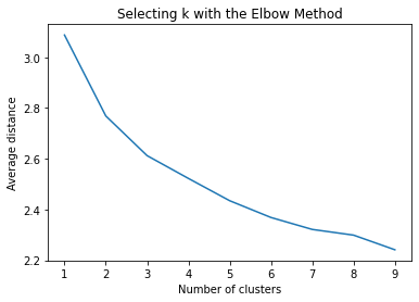
The dataset was randomly split into a training set (70%, N ≈ 29,165) and a test set (30%, N ≈ 12,493). K-means cluster analyses were performed on the training data using Euclidean distance, with solutions ranging from one to nine clusters. In Figure 1, t he average within-cluster distances were shown as an elbow curve. The elbow plot did not provide a clear point of inflection, but it did indicate that a 3-cluster solution may be a viable option for interpretation.
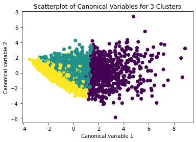
Canonical discriminant analysis was used to reduce the 12 clustering variables to two dimensions for visual purposes as shown in Figure 2. The scatterplot demonstrated that the three groups were slightly distinct in canonical space. Cluster 0 (the purple one) looked to be the biggest group, with more dense organizing, but clusters 1 and 2 (yellow and green) were smaller and more scattered, indicating more within-cluster variability.
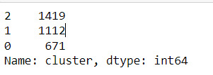
Descriptive statistics showed the cluster sizes: Cluster 0 (N=22,998), Cluster 1 (N=5,977), and Cluster 2 (N=1,190). Cluster 1 was characterized by above-average values in S1Q7A1, indicating higher engagement in the “present situation including working full time (35+ hour per week). and older age. Cluster 2 was differentiated by low values in S1Q7A8 and ADULTCH, suggesting more negative responses related to unemployed and permanently disabled present situation and adult child of respondent in the respondent’s household. Cluster 0 had mean values near the standardized average across most variables.
To externally validate the clusters, an ordinary least squares (OLS) regression was used to determine whether the clusters varied substantially in terms of drinking frequency (DRINKFREQ). The regression results suggested a statistically significant model (F(2, 17071) = 67.66, p < .0001), although the explained variance was modest (R² = 0.008). Post-hoc comparisons showed that Cluster 1 had a substantially greater drinking frequency (b = 0.0855, p <.0001) than Cluster 0, but Cluster 2 had a significantly lower drinking frequency (b = -0.0923, p <.0001). This validates the clusters' discriminant validity in terms of drinking habit.
These results indicates that self-reported drinking frequency varies according to different behavioral and demographic factors. Further investigation of the smallest cluster such as Cluster 2 may reveal protective variables or demographic traits associated with lower alcohol consumption.
Code:
from pandas import Series, DataFrame import pandas as pd import numpy as np import matplotlib.pyplot as plt from sklearn.model_selection import train_test_split from sklearn import preprocessing from sklearn.cluster import KMeans from sklearn.decomposition import PCA from scipy.spatial.distance import cdist import statsmodels.formula.api as smf import statsmodels.stats.multicomp as multi
""""Load dataset""" data = pd.read_csv("_358bd6a81b9045d95c894acf255c696a_nesarc_pds.csv")
""""Uppercase column names""" data.columns = map(str.upper, data.columns)
""""Drop missing values""" data_clean = data.dropna()
""""Subset clustering variables""" cluster = data_clean[['AGE', 'SEX', 'S1Q7A11', 'FMARITAL', 'S1Q7A1', 'S1Q7A8', 'S1Q7A9', 'S1Q7A2', 'S1Q7A3', 'ADULTCH', 'OTHREL', 'S1Q24LB']]
""""tandardize clustering variables""" clustervar = cluster.copy() for col in clustervar.columns: clustervar[col] = preprocessing.scale(clustervar[col].astype('float64'))
""""Split into training and testing sets""" clus_train, clus_test = train_test_split(clustervar, test_size=0.3, random_state=123)
""""K-means clustering with k from 1 to 9 (Elbow method)""" clusters = range(1, 10) meandist = []
for k in clusters: model = KMeans(n_clusters=k, random_state=123) model.fit(clus_train) meandist.append( sum(np.min(cdist(clus_train, model.cluster_centers_, 'euclidean'), axis=1)) / clus_train.shape[0] )
""""Plot Elbow Curve""" plt.figure() plt.plot(clusters, meandist, marker='o') plt.xlabel('Number of Clusters (k)') plt.ylabel('Average Distance to Centroid') plt.title('Elbow Method for Optimal k') plt.grid(True) plt.show()
"""" Fit KMeans for 3 clusters""" model3 = KMeans(n_clusters=3, random_state=123) model3.fit(clus_train) clusassign = model3.predict(clus_train)
""""visualization""" pca_2 = PCA(2) plot_columns = pca_2.fit_transform(clus_train) plt.figure() plt.scatter(x=plot_columns[:, 0], y=plot_columns[:, 1], c=model3.labels_, cmap='viridis') plt.xlabel('Canonical Variable 1') plt.ylabel('Canonical Variable 2') plt.title('Scatterplot of Canonical Variables for 3 Clusters') plt.grid(True) plt.show()
""""Merge cluster assignment with clustering variables""" clus_train.reset_index(level=0, inplace=True) cluslist = list(clus_train['index']) labels = list(model3.labels_) newlist = dict(zip(cluslist, labels)) newclus = DataFrame.from_dict(newlist, orient='index') newclus.columns = ['cluster'] newclus.reset_index(level=0, inplace=True) merged_train = pd.merge(clus_train, newclus, on='index')
""""Cluster frequencies""" print("Cluster sizes:") print(merged_train['cluster'].value_counts())
""""Cluster means""" clustergrp = merged_train.groupby('cluster').mean() print("Clustering variable means by cluster") print(clustergrp)
""""External validation using S2AQ21B - drinking frequency"""
""""Replace blanks and invalid codes"""" data['S2AQ21B'] = data['S2AQ21B'].replace([' ', 98, 99, 'BL'], pd.NA)
""""Drop rows with missing target values"""" data = data.dropna(subset=['S2AQ21B'])
""""Convert to numeric and recode binary target"""" data['S2AQ21B'] = data['S2AQ21B'].astype(int) data['DRINKFREQ'] = data['S2AQ21B'].apply(lambda x: 1 if x in [1, 2, 3, 4] else 0)
drinkfreq_data = data[['DRINKFREQ']] drinkfreq_train, drinkfreq_test = train_test_split(drinkfreq_data, test_size=0.3, random_state=123) drinkfreq_train1 = pd.DataFrame(drinkfreq_train) drinkfreq_train1.reset_index(level=0, inplace=True)
""""Merge with clustering data"""" merged_train_all = pd.merge(drinkfreq_train1, merged_train, on='index') sub1 = merged_train_all[['DRINKFREQ', 'cluster']].dropna()
"""" ANOVA to test cluster differences in DRINKFREQ"""" drinkmod = smf.ols(formula='DRINKFREQ ~ C(cluster)', data=sub1).fit() print(drinkmod.summary())
""""Means and SDs for DRINKFREQ by cluster"""" print('Means for DRINKFREQ by cluster') print(sub1.groupby('cluster').mean())
print('\nStandard deviations for DRINKFREQ by cluster') print(sub1.groupby('cluster').std())
""""Tukey HSD post-hoc test"""" mc1 = multi.MultiComparison(sub1['DRINKFREQ'], sub1['cluster']) res1 = mc1.tukeyhsd() print(res1.summary())
0 notes
Text
K-mean Analysis
Script:
from pandas import Series, DataFrame import pandas as pd import numpy as np import matplotlib.pylab as plt from sklearn.model_selection import train_test_split from sklearn import preprocessing from sklearn.cluster import KMeans import os """ Data Management """
data = pd.read_csv("tree_addhealth.csv")
upper-case all DataFrame column names
data.columns = map(str.upper, data.columns)
Data Management
data_clean = data.dropna()
subset clustering variables
cluster=data_clean[['ALCEVR1','MAREVER1','ALCPROBS1','DEVIANT1','VIOL1', 'DEP1','ESTEEM1','SCHCONN1','PARACTV', 'PARPRES','FAMCONCT']] cluster.describe()
standardize clustering variables to have mean=0 and sd=1
clustervar=cluster.copy() clustervar['ALCEVR1']=preprocessing.scale(clustervar['ALCEVR1'].astype('float64')) clustervar['ALCPROBS1']=preprocessing.scale(clustervar['ALCPROBS1'].astype('float64')) clustervar['MAREVER1']=preprocessing.scale(clustervar['MAREVER1'].astype('float64')) clustervar['DEP1']=preprocessing.scale(clustervar['DEP1'].astype('float64')) clustervar['ESTEEM1']=preprocessing.scale(clustervar['ESTEEM1'].astype('float64')) clustervar['VIOL1']=preprocessing.scale(clustervar['VIOL1'].astype('float64')) clustervar['DEVIANT1']=preprocessing.scale(clustervar['DEVIANT1'].astype('float64')) clustervar['FAMCONCT']=preprocessing.scale(clustervar['FAMCONCT'].astype('float64')) clustervar['SCHCONN1']=preprocessing.scale(clustervar['SCHCONN1'].astype('float64')) clustervar['PARACTV']=preprocessing.scale(clustervar['PARACTV'].astype('float64')) clustervar['PARPRES']=preprocessing.scale(clustervar['PARPRES'].astype('float64'))
split data into train and test sets
clus_train, clus_test = train_test_split(clustervar, test_size=.3, random_state=123)
k-means cluster analysis for 1-9 clusters
from scipy.spatial.distance import cdist clusters=range(1,9) meandist=[]
for k in clusters: model=KMeans(n_clusters=k) model.fit(clus_train) clusassign=model.predict(clus_train) meandist.append(sum(np.min(cdist(clus_train, model.cluster_centers_, 'euclidean'), axis=1)) / clus_train.shape[0])
""" Plot average distance from observations from the cluster centroid to use the Elbow Method to identify number of clusters to choose """
plt.plot(clusters, meandist) plt.xlabel('Number of clusters') plt.ylabel('Average distance') plt.title('Selecting k with the Elbow Method')
Interpret 3 cluster solution
model3=KMeans(n_clusters=2) model3.fit(clus_train) clusassign=model3.predict(clus_train)
plot clusters
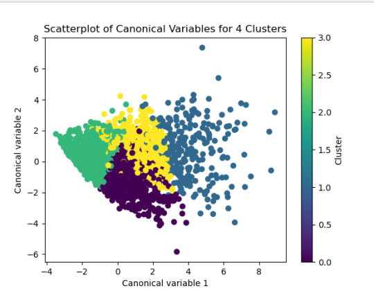
from sklearn.decomposition import PCA pca_2 = PCA(2) plot_columns = pca_2.fit_transform(clus_train) plt.scatter(x=plot_columns[:,0], y=plot_columns[:,1], c=model3.labels_) plt.xlabel('Canonical variable 1') plt.ylabel('Canonical variable 2') plt.title('Scatterplot of Canonical Variables for 4 Clusters')
Add the legend to the plot
import matplotlib.patches as mpatches patches = [mpatches.Patch(color=plt.cm.viridis(i/4), label=f'Cluster {i}') for i in range(4)]
plt.legend(handles=patches, title="Clusters") plt.show()
""" BEGIN multiple steps to merge cluster assignment with clustering variables to examine cluster variable means by cluster """
create a unique identifier variable from the index for the
cluster training data to merge with the cluster assignment variable
clus_train.reset_index(level=0, inplace=True)
create a list that has the new index variable
cluslist=list(clus_train['index'])
create a list of cluster assignments
labels=list(model3.labels_)
combine index variable list with cluster assignment list into a dictionary
newlist=dict(zip(cluslist, labels)) newlist
convert newlist dictionary to a dataframe
newclus=DataFrame.from_dict(newlist, orient='index') newclus
rename the cluster assignment column
newclus.columns = ['cluster']
now do the same for the cluster assignment variable
create a unique identifier variable from the index for the
cluster assignment dataframe
to merge with cluster training data
newclus.reset_index(level=0, inplace=True)
merge the cluster assignment dataframe with the cluster training variable dataframe
by the index variable
merged_train=pd.merge(clus_train, newclus, on='index') merged_train.head(n=100)
cluster frequencies
merged_train.cluster.value_counts()
""" END multiple steps to merge cluster assignment with clustering variables to examine cluster variable means by cluster """
FINALLY calculate clustering variable means by cluster
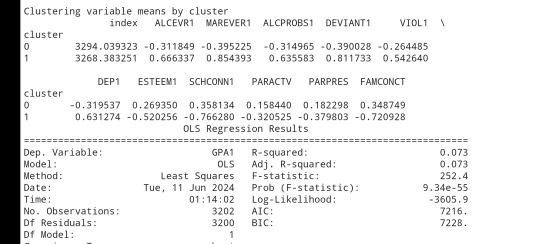
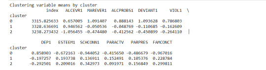
clustergrp = merged_train.groupby('cluster').mean() print ("Clustering variable means by cluster") print(clustergrp)
validate clusters in training data by examining cluster differences in GPA using ANOVA
first have to merge GPA with clustering variables and cluster assignment data
gpa_data=data_clean['GPA1']
split GPA data into train and test sets
gpa_train, gpa_test = train_test_split(gpa_data, test_size=.3, random_state=123) gpa_train1=pd.DataFrame(gpa_train) gpa_train1.reset_index(level=0, inplace=True) merged_train_all=pd.merge(gpa_train1, merged_train, on='index') sub1 = merged_train_all[['GPA1', 'cluster']].dropna()
import statsmodels.formula.api as smf import statsmodels.stats.multicomp as multi
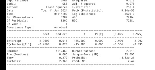
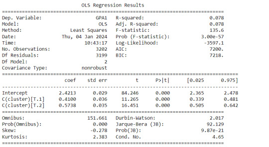
gpamod = smf.ols(formula='GPA1 ~ C(cluster)', data=sub1).fit() print (gpamod.summary())
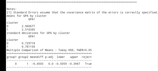
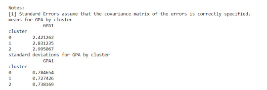
print ('means for GPA by cluster') m1= sub1.groupby('cluster').mean() print (m1)
print ('standard deviations for GPA by cluster') m2= sub1.groupby('cluster').std() print (m2)
mc1 = multi.MultiComparison(sub1['GPA1'], sub1['cluster']) res1 = mc1.tukeyhsd() print(res1.summary())
------------------------------------------------------------------------------
PLOTS:

------------------------------------------------------------------------------ANALYSING:
The K-mean cluster analysis is trying to identify subgroups of adolescents based on their similarity using the following 11 variables:
(Binary variables)
ALCEVR1 = ever used alcohol
MAREVER1 = ever used marijuana
(Quantitative variables)
ALCPROBS1 = Alcohol problem
DEVIANT1 = behaviors scale
VIOL1 = Violence scale
DEP1 = depression scale
ESTEEM1 = Self-esteem
SCHCONN1= School connectiveness
PARACTV = parent activities
PARPRES = parent presence
FAMCONCT = family connectiveness
The test was split with 70% for the training set and 30% for the test set. 9 clusters were conducted and the results are shown the plot 1. The plot suggest 2,4 , 5 and 6 solutions might be interpreted.
The second plot shows the canonical discriminant analyses of the 4 cluster solutions. Clusters 0 and 3 are very densely packed together with relatively low within-cluster variance whereas clusters 1 and 2 were spread out more than the other clusters, especially cluster 1 which means there is higher variance within the cluster. The number of clusters we would need to use is less the 3.


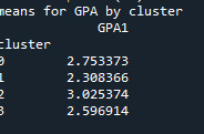
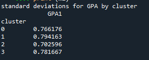

Students in cluster 2 had higher GPA values with an SD of 0.70 and cluster 1 had lower GPA values with an SD of 0.79
0 notes
Text
Data Visualization - Assignment 2
For my first Python program, please see below:
-----------------------------PROGRAM--------------------------------
-- coding: utf-8 --
""" Created: 27FEB2025
@author:Nicole taylor """ import pandas import numpy
any additional libraries would be imported here
data = pandas.read_csv('GapFinder- _PDS.csv', low_memory=False)
print (len(data)) #number of observations (rows) print (len(data.columns)) # number of variables (columns)
checking the format of your variables
data['ref_area.label'].dtype
setting variables you will be working with to numeric
data['obs_value'] = pandas.to_numeric(data['obs_value'])
counts and percentages (i.e. frequency distributions) for each variable
Value1 = data['obs_value'].value_counts(sort=False) print (Value1)
PValue1 = data['obs_value'].value_counts(sort=False, normalize=True) print (PValue1)
Gender = data['sex.label'].value_counts(sort=False) print (Gender)
PGender = data['sex.label'].value_counts(sort=False, normalize=True) print (PGender)
Country = data['Country.label'].value_counts(sort=False) print (Country)
PCountry = data['Country.label'].value_counts(sort=False, normalize=True) print (PCountry)
MStatus = data['MaritalStatus.label'].value_counts(sort=False) print (MStatus)
PMStatus = data['MaritalStatus.label'].value_counts(sort=False, normalize=True) print (PMStatus)
LMarket = data['LaborMarket.label'].value_counts(sort=False) print (LMarket)
PLMarket = data['LaborMarket.label'].value_counts(sort=False, normalize=True) print (PLMarket)
Year = data['Year.label'].value_counts(sort=False) print (Year)
PYear = data['Year.label'].value_counts(sort=False, normalize=True) print (PYear)
ADDING TITLES
print ('counts for Value') Value1 = data['obs_value'].value_counts(sort=False) print (Value1)
print (len(data['TAB12MDX'])) #number of observations (rows)
print ('percentages for Value') p1 = data['obs_value'].value_counts(sort=False, normalize=True) print (PValue1)
print ('counts for Gender') Gender = data['sex.label'].value_counts(sort=False) print(Gender)
print ('percentages for Gender') p2 = data['sex.label'].value_counts(sort=False, normalize=True) print (PGender)
print ('counts for Country') Country = data['Country.label'].value_counts(sort=False, dropna=False) print(Country)
print ('percentages for Country') PCountry = data['Country.label'].value_counts(sort=False, normalize=True) print (PCountry)
print ('counts for Marital Status') MStatus = data['MaritalStatus.label'].value_counts(sort=False, dropna=False) print(MStatus)
print ('percentages for Marital Status') PMStatus = data['MaritalStatus.label'].value_counts(sort=False, dropna=False, normalize=True) print (PMStatus)
print ('counts for Labor Market') LMarket = data['LaborMarket.label'].value_counts(sort=False, dropna=False) print(LMarket)
print ('percentages for Labor Market') PLMarket = data['LaborMarket.label'].value_counts(sort=False, dropna=False, normalize=True) print (PLMarket)
print ('counts for Year') Year = data['Year.label'].value_counts(sort=False, dropna=False) print(Year)
print ('percentages for Year') PYear = data['Year.label'].value_counts(sort=False, dropna=False, normalize=True) print (PYear)
---------------------------------------------------------------------------
frequency distributions using the 'bygroup' function
print ('Frequency of Countries') TCountry = data.groupby('Country.label').size() print(TCountry)
subset data to young adults age 18 to 25 who have smoked in the past 12 months
sub1=data[(data[TCountry]='United States of America') & (data[Gender]='Sex:Female')]
make a copy of my new subsetted data
sub2 = sub1.copy()
frequency distributions on new sub2 data frame
print('counts for Country')
c5 = sub1['Country.label'].value_counts(sort=False)
print(c5)
upper-case all DataFrame column names - place afer code for loading data aboave
data.columns = list(map(str.upper, data.columns))
bug fix for display formats to avoid run time errors - put after code for loading data above
pandas.set_option('display.float_format', lambda x:'%f'%x)
-----------------------------RESULTS--------------------------------
runcell(0, 'C:/Users/oen8fh/.spyder-py3/temp.py') 85856 12 16372.131 1 7679.474 1 462.411 1 8230.246 1 4758.121 1 .. 1609.572 1 95.113 1 372.197 1 8.814 1 3.796 1 Name: obs_value, Length: 79983, dtype: int64
16372.131 0.000012 7679.474 0.000012 462.411 0.000012 8230.246 0.000012 4758.121 0.000012
1609.572 0.000012 95.113 0.000012 372.197 0.000012 8.814 0.000012 3.796 0.000012 Name: obs_value, Length: 79983, dtype: float64
Sex: Total 28595 Sex: Male 28592 Sex: Female 28595 Sex: Other 74 Name: sex.label, dtype: int64 Sex: Total 0.333058 Sex: Male 0.333023 Sex: Female 0.333058 Sex: Other 0.000862 Name: sex.label, dtype: float64 Afghanistan 210 Angola 291 Albania 696 Argentina 768 Armenia 627
Samoa 117 Yemen 36 South Africa 993 Zambia 306 Zimbabwe 261 Name: Country.label, Length: 169, dtype: int64
Afghanistan 0.002446 Angola 0.003389 Albania 0.008107 Argentina 0.008945 Armenia 0.007303
Samoa 0.001363 Yemen 0.000419 South Africa 0.011566 Zambia 0.003564 Zimbabwe 0.003040 Name: Country.label, Length: 169, dtype: float64
Marital status (Aggregate): Total 26164 Marital status (Aggregate): Single / Widowed / Divorced 26161 Marital status (Aggregate): Married / Union / Cohabiting 26156 Marital status (Aggregate): Not elsewhere classified 7375 Name: MaritalStatus.label, dtype: int64
Marital status (Aggregate): Total 0.304743 Marital status (Aggregate): Single / Widowed / Divorced 0.304708 Marital status (Aggregate): Married / Union / Cohabiting 0.304650 Marital status (Aggregate): Not elsewhere classified 0.085900 Name: MaritalStatus.label, dtype: float64
Labour market status: Total 21870 Labour market status: Employed 21540 Labour market status: Unemployed 20736 Labour market status: Outside the labour force 21710 Name: LaborMarket.label, dtype: int64
Labour market status: Total 0.254729 Labour market status: Employed 0.250885 Labour market status: Unemployed 0.241521 Labour market status: Outside the labour force 0.252865 Name: LaborMarket.label, dtype: float64
2021 3186 2020 3641 2017 4125 2014 4014 2012 3654 2022 3311 2019 4552 2011 3522 2009 3054 2004 2085 2023 2424 2018 3872 2016 3843 2015 3654 2013 3531 2010 3416 2008 2688 2007 2613 2005 2673 2002 1935 2006 2700 2024 372 2003 2064 2001 1943 2000 1887 1999 1416 1998 1224 1997 1086 1996 999 1995 810 1994 714 1993 543 1992 537 1991 594 1990 498 1989 462 1988 423 1987 423 1986 357 1985 315 1984 273 1983 309 1982 36 1980 36 1970 42 Name: Year.label, dtype: int64
2021 0.037109 2020 0.042408 2017 0.048046 2014 0.046753 2012 0.042560 2022 0.038565 2019 0.053019 2011 0.041022 2009 0.035571 2004 0.024285 2023 0.028233 2018 0.045099 2016 0.044761 2015 0.042560 2013 0.041127 2010 0.039788 2008 0.031308 2007 0.030435 2005 0.031134 2002 0.022538 2006 0.031448 2024 0.004333 2003 0.024040 2001 0.022631 2000 0.021979 1999 0.016493 1998 0.014256 1997 0.012649 1996 0.011636 1995 0.009434 1994 0.008316 1993 0.006325 1992 0.006255 1991 0.006919 1990 0.005800 1989 0.005381 1988 0.004927 1987 0.004927 1986 0.004158 1985 0.003669 1984 0.003180 1983 0.003599 1982 0.000419 1980 0.000419 1970 0.000489 Name: Year.label, dtype: float64
counts for Value 16372.131 1 7679.474 1 462.411 1 8230.246 1 4758.121 1 .. 1609.572 1 95.113 1 372.197 1 8.814 1 3.796 1 Name: obs_value, Length: 79983, dtype: int64
percentages for Value 16372.131 0.000012 7679.474 0.000012 462.411 0.000012 8230.246 0.000012 4758.121 0.000012
1609.572 0.000012 95.113 0.000012 372.197 0.000012 8.814 0.000012 3.796 0.000012 Name: obs_value, Length: 79983, dtype: float64
counts for Gender Sex: Total 28595 Sex: Male 28592 Sex: Female 28595 Sex: Other 74 Name: sex.label, dtype: int64
percentages for Gender Sex: Total 0.333058 Sex: Male 0.333023 Sex: Female 0.333058 Sex: Other 0.000862 Name: sex.label, dtype: float64
counts for Country Afghanistan 210 Angola 291 Albania 696 Argentina 768 Armenia 627
Samoa 117 Yemen 36 South Africa 993 Zambia 306 Zimbabwe 261 Name: Country.label, Length: 169, dtype: int64
percentages for Country Afghanistan 0.002446 Angola 0.003389 Albania 0.008107 Argentina 0.008945 Armenia 0.007303
Samoa 0.001363 Yemen 0.000419 South Africa 0.011566 Zambia 0.003564 Zimbabwe 0.003040 Name: Country.label, Length: 169, dtype: float64
counts for Marital Status Marital status (Aggregate): Total 26164 Marital status (Aggregate): Single / Widowed / Divorced 26161 Marital status (Aggregate): Married / Union / Cohabiting 26156 Marital status (Aggregate): Not elsewhere classified 7375 Name: MaritalStatus.label, dtype: int64
percentages for Marital Status Marital status (Aggregate): Total 0.304743 Marital status (Aggregate): Single / Widowed / Divorced 0.304708 Marital status (Aggregate): Married / Union / Cohabiting 0.304650 Marital status (Aggregate): Not elsewhere classified 0.085900 Name: MaritalStatus.label, dtype: float64
counts for Labor Market Labour market status: Total 21870 Labour market status: Employed 21540 Labour market status: Unemployed 20736 Labour market status: Outside the labour force 21710 Name: LaborMarket.label, dtype: int64
percentages for Labor Market Labour market status: Total 0.254729 Labour market status: Employed 0.250885 Labour market status: Unemployed 0.241521 Labour market status: Outside the labour force 0.252865 Name: LaborMarket.label, dtype: float64
counts for Year 2021 3186 2020 3641 2017 4125 2014 4014 2012 3654 2022 3311 2019 4552 2011 3522 2009 3054 2004 2085 2023 2424 2018 3872 2016 3843 2015 3654 2013 3531 2010 3416 2008 2688 2007 2613 2005 2673 2002 1935 2006 2700 2024 372 2003 2064 2001 1943 2000 1887 1999 1416 1998 1224 1997 1086 1996 999 1995 810 1994 714 1993 543 1992 537 1991 594 1990 498 1989 462 1988 423 1987 423 1986 357 1985 315 1984 273 1983 309 1982 36 1980 36 1970 42 Name: Year.label, dtype: int64
percentages for Year 2021 0.037109 2020 0.042408 2017 0.048046 2014 0.046753 2012 0.042560 2022 0.038565 2019 0.053019 2011 0.041022 2009 0.035571 2004 0.024285 2023 0.028233 2018 0.045099 2016 0.044761 2015 0.042560 2013 0.041127 2010 0.039788 2008 0.031308 2007 0.030435 2005 0.031134 2002 0.022538 2006 0.031448 2024 0.004333 2003 0.024040 2001 0.022631 2000 0.021979 1999 0.016493 1998 0.014256 1997 0.012649 1996 0.011636 1995 0.009434 1994 0.008316 1993 0.006325 1992 0.006255 1991 0.006919 1990 0.005800 1989 0.005381 1988 0.004927 1987 0.004927 1986 0.004158 1985 0.003669 1984 0.003180 1983 0.003599 1982 0.000419 1980 0.000419 1970 0.000489 Name: Year.label, dtype: float64
Frequency of Countries Country.label Afghanistan 210 Albania 696 Angola 291 Antigua and Barbuda 87 Argentina 768
Viet Nam 639 Wallis and Futuna 117 Yemen 36 Zambia 306 Zimbabwe 261 Length: 169, dtype: int64
-----------------------------REVIEW--------------------------------
So as you can see in the results. I was able to show the Year, Marital Status, Labor Market, and the Country. I'm still a little hazy on the sub1, but overall it was a good basic start.
0 notes
Text
BigQuery DataFrame And Gretel Verify Synthetic Data Privacy

It looked at how combining Gretel with BigQuery DataFrame simplifies synthetic data production while maintaining data privacy in the useful guide to synthetic data generation with Gretel and BigQuery DataFrames. In summary, BigQuery DataFrame is a Python client for BigQuery that offers analysis pushed down to BigQuery using pandas-compatible APIs.
Gretel provides an extensive toolkit for creating synthetic data using state-of-the-art machine learning methods, such as large language models (LLMs). An seamless workflow is made possible by this integration, which makes it simple for users to move data from BigQuery to Gretel and return the created results to BigQuery.
The technical elements of creating synthetic data to spur AI/ML innovation are covered in detail in this tutorial, along with tips for maintaining high data quality, protecting privacy, and adhering to privacy laws. In Part 1, to de-identify the data from a BigQuery patient records table, and in Part 2, it create synthetic data to be saved back to BigQuery.
Setting the stage: Installation and configuration
With BigFrames already installed, you may begin by using BigQuery Studio as the notebook runtime. To presume you are acquainted with Pandas and have a Google Cloud project set up.
Step 1: Set up BigQuery DataFrame and the Gretel Python client.
Step 2: Set up BigFrames and the Gretel SDK: To use their services, you will want a Gretel API key. One is available on the Gretel console.
Part 1: De-identifying and processing data with Gretel Transform v2
De-identifying personally identifiable information (PII) is an essential initial step in data anonymization before creating synthetic data. For these and other data processing tasks, Gretel Transform v2 (Tv2) offers a strong and expandable framework.
Tv2 handles huge datasets efficiently by combining named entity recognition (NER) skills with sophisticated transformation algorithms. Tv2 is a flexible tool in the data preparation pipeline as it may be used for preprocessing, formatting, and data cleaning in addition to PII de-identification. Study up on Gretel Transform v2.
Step 1: Convert your BigQuery table into a BigFrames DataFrame.
Step 2: Work with Gretel to transform the data.
Part 2: Generating synthetic data with Navigator Fine Tuning (LLM-based)
Gretel Navigator Fine Tuning (NavFT) refines pre-trained models on your datasets to provide high-quality, domain-specific synthetic data. Important characteristics include:
Manages a variety of data formats, including time series, JSON, free text, category, and numerical.
Maintains intricate connections between rows and data kinds.
May provide significant novel patterns, which might enhance the performance of ML/AI tasks.
Combines privacy protection with data usefulness.
By utilizing the advantages of domain-specific pre-trained models, NavFT expands on Gretel Navigator’s capabilities and makes it possible to create synthetic data that captures the subtleties of your particular data, such as the distributions and correlations for numeric, categorical, and other column types.
Using the de-identified data from Part 1, it will refine a Gretel model in this example.
Step 1: Make a model better:
# Display the full report within this notebooktrain_results.report.display_in_notebook()
Step 2: Retrieve the Quality Report for Gretel Synthetic Data.
Step 3: Create synthetic data using the optimized model, assess the privacy and quality of the data, and then publish the results back to a BQ table.
A few things to note about the synthetic data:
Semantically accurate, the different modalities (free text, JSON structures) are completely synthetic and retained.
The data are grouped by patient during creation due to the group-by/order-by hyperparameters that were used during fine-tuning.
How to use BigQuery with Gretel
This technical manual offers a starting point for creating and using synthetic data using Gretel AI and BigQuery DataFrame. You may use the potential of synthetic data to improve your data science, analytics, and artificial intelligence development processes while maintaining data privacy and compliance by examining the Gretel documentation and using these examples.
Read more on Govindhtech.com
#BigQueryDataFrame#DataFrame#Gretel#AI#ML#Python#SyntheticData#cloudcomputing#BigQuery#News#Technews#Technology#Technologynews#Technologytrends#govindhtech
0 notes
Text
K-means clusthering
#importamos las librerías necesarias
from pandas import Series,DataFrame
import pandas as pd
import numpy as np
import matplotlib.pylab as plt
from sklearn.model_selection
import train_test_splitfrom sklearn
import preprocessing
from sklearn.cluster import KMeans
"""Data Management"""
data =pd.read_csv("/content/drive/MyDrive/tree_addhealth.csv" )
#upper-case all DataFrame column names
data.columns = map(str.upper, data.columns)
# Data Managementdata_clean = data.dropna()
# subset clustering variablescluster=data_clean[['ALCEVR1','MAREVER1','ALCPROBS1','DEVIANT1','VIOL1','DEP1','ESTEEM1','SCHCONN1','PARACTV', 'PARPRES','FAMCONCT']]
cluster.describe()
# standardize clustering variables to have mean=0 and sd=1
clustervar=cluster.copy()
clustervar['ALCEVR1']=preprocessing.scale(clustervar['ALCEVR1'].astype('float64'))
clustervar['ALCPROBS1']=preprocessing.scale(clustervar['ALCPROBS1'].astype('float64'))
clustervar['MAREVER1']=preprocessing.scale(clustervar['MAREVER1'].astype('float64'))
clustervar['DEP1']=preprocessing.scale(clustervar['DEP1'].astype('float64'))
clustervar['ESTEEM1']=preprocessing.scale(clustervar['ESTEEM1'].astype('float64'))
clustervar['VIOL1']=preprocessing.scale(clustervar['VIOL1'].astype('float64'))
clustervar['DEVIANT1']=preprocessing.scale(clustervar['DEVIANT1'].astype('float64'))
clustervar['FAMCONCT']=preprocessing.scale(clustervar['FAMCONCT'].astype('float64'))
clustervar['SCHCONN1']=preprocessing.scale(clustervar['SCHCONN1'].astype('float64'))
clustervar['PARACTV']=preprocessing.scale(clustervar['PARACTV'].astype('float64'))
clustervar['PARPRES']=preprocessing.scale(clustervar['PARPRES'].astype('float64'))
# split data into train and test sets
clus_train, clus_test = train_test_split(clustervar, test_size=.3, random_state=123)
# k-means cluster analysis for 1-9 clusters
from scipy.spatial.distance import cdist
clusters=range(1,10)
meandist=[]
for k in clusters: model=KMeans(n_clusters=k) model.fit(clus_train) clusassign=model.predict(clus_train) meandist.append(sum(np.min(cdist(clus_train, model.cluster_centers_, 'euclidean'), axis=1))
/ clus_train.shape[0])
"""Plot average distance from observations from the cluster centroidto use the Elbow Method to identify number of clusters to choose"""
plt.plot(clusters,meandist)
plt.xlabel('Number of clusters')
plt.ylabel('Average distance')
plt.title('Selecting k with the Elbow Method')
# Interpret 2 cluster solution
model2=KMeans(n_clusters=2)model2.fit(clus_train)
clusassign=model2.predict(clus_train)
# plot clusters
from sklearn.decomposition import PCA
pca_2 = PCA(2)
plot_columns = pca_2.fit_transform(clus_train)
plt.scatter(x=plot_columns[:,0],y=plot_columns[:,1],c=model2.labels_,)
plt.xlabel('Canonical variable 1')
plt.ylabel('Canonical variable 2')
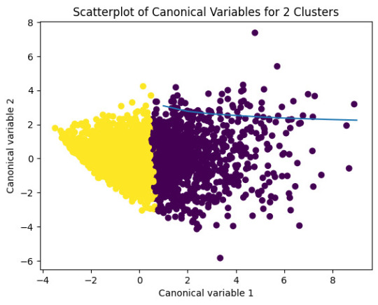
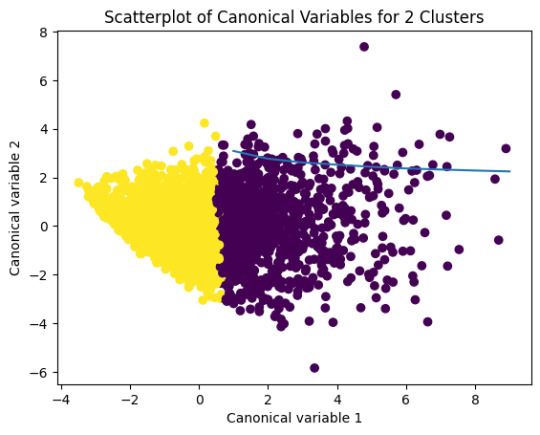
plt.title('Scatterplot of Canonical Variables for 2 Clusters')
plt.show()
"""BEGIN multiple steps to merge cluster assignment with clustering variables to examinecluster variable means by cluster"""
# create a unique identifier variable from the index for the
# cluster training data to merge with the cluster assignment variable
clus_train.reset_index(level=0, inplace=True)
# create a list that has the new index variable
cluslist=list(clus_train['index'])
# create a list of cluster assignments
labels=list(model2.labels_)
# combine index variable list with cluster assignment list into a dictionary
newlist=dict(zip(cluslist, labels))newlist
# convert newlist dictionary to a dataframenew
clus=DataFrame.from_dict(newlist, orient='index')newclus
# rename the cluster assignment columnnew
clus.columns = ['cluster']
# now do the same for the cluster assignment variable
# create a unique identifier variable from the index for the
# cluster assignment dataframe
# to merge with cluster training datanew
clus.reset_index(level=0, inplace=True)
# merge the cluster assignment dataframe with the cluster training variable dataframe
# by the index variablemerged_train=pd.merge(clus_train, newclus, on='index')
merged_train.head(n=100)
# cluster frequenciesmerged_train.cluster.value_counts()
"""END multiple steps to merge cluster assignment with clustering variables to examinecluster variable means by cluster"""
# FINALLY calculate clustering variable means by
clusterclustergrp = merged_train.groupby('cluster').mean()print ("Clustering variable means by cluster")
print(clustergrp)
# validate clusters in training data by examining cluster differences in GPA using ANOVA
# first have to merge GPA with clustering variables and cluster assignment data
gpa_data=data_clean['GPA1']
# split GPA data into train and test sets
gpa_train, gpa_test = train_test_split(gpa_data, test_size=.3, random_state=123)
gpa_train1=pd.DataFrame(gpa_train)
gpa_train1.reset_index(level=0, inplace=True)
merged_train_all=pd.merge(gpa_train1, merged_train, on='index')
sub1 = merged_train_all[['GPA1', 'cluster']].dropna()
import statsmodels.formula.api as smf
import statsmodels.stats.multicomp as multi
gpamod = smf.ols(formula='GPA1 ~ C(cluster)', data=sub1).fit()
print (gpamod.summary())
print ('means for GPA by cluster')
m1= sub1.groupby('cluster').mean()
print (m1)
print ('standard deviations for GPA by cluster')
m2= sub1.groupby('cluster').std()print (m2)
mc1 = multi.MultiComparison(sub1['GPA1'], sub1['cluster'])
res1 = mc1.tukeyhsd()
print(res1.summary())
爆發
0 則迴響
0 notes
Text
K-means clusthering
#importamos las librerías necesarias
from pandas import Series,DataFrame
import pandas as pd
import numpy as np
import matplotlib.pylab as plt
from sklearn.model_selection
import train_test_splitfrom sklearn
import preprocessing
from sklearn.cluster import KMeans
"""Data Management"""
data =pd.read_csv("/content/drive/MyDrive/tree_addhealth.csv" )
#upper-case all DataFrame column names
data.columns = map(str.upper, data.columns)
# Data Managementdata_clean = data.dropna()
# subset clustering variablescluster=data_clean[['ALCEVR1','MAREVER1','ALCPROBS1','DEVIANT1','VIOL1','DEP1','ESTEEM1','SCHCONN1','PARACTV', 'PARPRES','FAMCONCT']]
cluster.describe()
# standardize clustering variables to have mean=0 and sd=1
clustervar=cluster.copy()
clustervar['ALCEVR1']=preprocessing.scale(clustervar['ALCEVR1'].astype('float64'))
clustervar['ALCPROBS1']=preprocessing.scale(clustervar['ALCPROBS1'].astype('float64'))
clustervar['MAREVER1']=preprocessing.scale(clustervar['MAREVER1'].astype('float64'))
clustervar['DEP1']=preprocessing.scale(clustervar['DEP1'].astype('float64'))
clustervar['ESTEEM1']=preprocessing.scale(clustervar['ESTEEM1'].astype('float64'))
clustervar['VIOL1']=preprocessing.scale(clustervar['VIOL1'].astype('float64'))
clustervar['DEVIANT1']=preprocessing.scale(clustervar['DEVIANT1'].astype('float64'))
clustervar['FAMCONCT']=preprocessing.scale(clustervar['FAMCONCT'].astype('float64'))
clustervar['SCHCONN1']=preprocessing.scale(clustervar['SCHCONN1'].astype('float64'))
clustervar['PARACTV']=preprocessing.scale(clustervar['PARACTV'].astype('float64'))
clustervar['PARPRES']=preprocessing.scale(clustervar['PARPRES'].astype('float64'))
# split data into train and test sets
clus_train, clus_test = train_test_split(clustervar, test_size=.3, random_state=123)
# k-means cluster analysis for 1-9 clusters
from scipy.spatial.distance import cdist
clusters=range(1,10)
meandist=[]
for k in clusters: model=KMeans(n_clusters=k) model.fit(clus_train) clusassign=model.predict(clus_train) meandist.append(sum(np.min(cdist(clus_train, model.cluster_centers_, 'euclidean'), axis=1))
/ clus_train.shape[0])
"""Plot average distance from observations from the cluster centroidto use the Elbow Method to identify number of clusters to choose"""
plt.plot(clusters,meandist)
plt.xlabel('Number of clusters')
plt.ylabel('Average distance')
plt.title('Selecting k with the Elbow Method')
# Interpret 2 cluster solution
model2=KMeans(n_clusters=2)model2.fit(clus_train)
clusassign=model2.predict(clus_train)
# plot clusters
from sklearn.decomposition import PCA
pca_2 = PCA(2)
plot_columns = pca_2.fit_transform(clus_train)
plt.scatter(x=plot_columns[:,0],y=plot_columns[:,1],c=model2.labels_,)
plt.xlabel('Canonical variable 1')
plt.ylabel('Canonical variable 2')
plt.title('Scatterplot of Canonical Variables for 2 Clusters')
plt.show()
"""BEGIN multiple steps to merge cluster assignment with clustering variables to examinecluster variable means by cluster"""
# create a unique identifier variable from the index for the
# cluster training data to merge with the cluster assignment variable
clus_train.reset_index(level=0, inplace=True)
# create a list that has the new index variable
cluslist=list(clus_train['index'])
# create a list of cluster assignments
labels=list(model2.labels_)
# combine index variable list with cluster assignment list into a dictionary
newlist=dict(zip(cluslist, labels))newlist
# convert newlist dictionary to a dataframenew
clus=DataFrame.from_dict(newlist, orient='index')newclus
# rename the cluster assignment columnnew
clus.columns = ['cluster']
# now do the same for the cluster assignment variable
# create a unique identifier variable from the index for the
# cluster assignment dataframe
# to merge with cluster training datanew
clus.reset_index(level=0, inplace=True)
# merge the cluster assignment dataframe with the cluster training variable dataframe
# by the index variablemerged_train=pd.merge(clus_train, newclus, on='index')
merged_train.head(n=100)
# cluster frequenciesmerged_train.cluster.value_counts()
"""END multiple steps to merge cluster assignment with clustering variables to examinecluster variable means by cluster"""
# FINALLY calculate clustering variable means by
clusterclustergrp = merged_train.groupby('cluster').mean()print ("Clustering variable means by cluster")
print(clustergrp)
# validate clusters in training data by examining cluster differences in GPA using ANOVA
# first have to merge GPA with clustering variables and cluster assignment data
gpa_data=data_clean['GPA1']
# split GPA data into train and test sets
gpa_train, gpa_test = train_test_split(gpa_data, test_size=.3, random_state=123)
gpa_train1=pd.DataFrame(gpa_train)
gpa_train1.reset_index(level=0, inplace=True)
merged_train_all=pd.merge(gpa_train1, merged_train, on='index')
sub1 = merged_train_all[['GPA1', 'cluster']].dropna()
import statsmodels.formula.api as smf
import statsmodels.stats.multicomp as multi
gpamod = smf.ols(formula='GPA1 ~ C(cluster)', data=sub1).fit()
print (gpamod.summary())
print ('means for GPA by cluster')
m1= sub1.groupby('cluster').mean()
print (m1)
print ('standard deviations for GPA by cluster')
m2= sub1.groupby('cluster').std()print (m2)
mc1 = multi.MultiComparison(sub1['GPA1'], sub1['cluster'])
res1 = mc1.tukeyhsd()
print(res1.summary())
0 notes
Text
weight of smokers
import pandas as pd import numpy as np
Read the dataset
data = pd.read_csv('nesarc_pds.csv', low_memory=False)
Bug fix for display formats to avoid runtime errors
pd.set_option('display.float_format', lambda x: '%f' % x)
Setting variables to numeric
numeric_columns = ['TAB12MDX', 'CHECK321', 'S3AQ3B1', 'S3AQ3C1', 'WEIGHT'] data[numeric_columns] = data[numeric_columns].apply(pd.to_numeric)
Subset data to adults 100 to 600 lbs who have smoked in the past 12 months
sub1 = data[(data['WEIGHT'] >= 100) & (data['WEIGHT'] <= 600) & (data['CHECK321'] == 1)]
Make a copy of the subsetted data
sub2 = sub1.copy()
def print_value_counts(df, column, description): """Print value counts for a specific column in the dataframe.""" print(f'{description}') counts = df[column].value_counts(sort=False, dropna=False) print(counts) return counts
Initial counts for S3AQ3B1
print_value_counts(sub2, 'S3AQ3B1', 'Counts for original S3AQ3B1')
Recode missing values to NaN
sub2['S3AQ3B1'].replace(9, np.nan, inplace=True) sub2['S3AQ3C1'].replace(99, np.nan, inplace=True)
Counts after recoding missing values
print_value_counts(sub2, 'S3AQ3B1', 'Counts for S3AQ3B1 with 9 set to NaN and number of missing requested')
Recode missing values for S2AQ8A
sub2['S2AQ8A'].fillna(11, inplace=True) sub2['S2AQ8A'].replace(99, np.nan, inplace=True)
Check coding for S2AQ8A
print_value_counts(sub2, 'S2AQ8A', 'S2AQ8A with Blanks recoded as 11 and 99 set to NaN') print(sub2['S2AQ8A'].describe())
Recode values for S3AQ3B1 into new variables
recode1 = {1: 6, 2: 5, 3: 4, 4: 3, 5: 2, 6: 1} recode2 = {1: 30, 2: 22, 3: 14, 4: 5, 5: 2.5, 6: 1}
sub2['USFREQ'] = sub2['S3AQ3B1'].map(recode1) sub2['USFREQMO'] = sub2['S3AQ3B1'].map(recode2)
Create secondary variable
sub2['NUMCIGMO_EST'] = sub2['USFREQMO'] * sub2['S3AQ3C1']
Examine frequency distributions for WEIGHT
print_value_counts(sub2, 'WEIGHT', 'Counts for WEIGHT') print('Percentages for WEIGHT') print(sub2['WEIGHT'].value_counts(sort=False, normalize=True))
Quartile split for WEIGHT
sub2['WEIGHTGROUP4'] = pd.qcut(sub2['WEIGHT'], 4, labels=["1=0%tile", "2=25%tile", "3=50%tile", "4=75%tile"]) print_value_counts(sub2, 'WEIGHTGROUP4', 'WEIGHT - 4 categories - quartiles')
Categorize WEIGHT into 3 groups (100-200 lbs, 200-300 lbs, 300-600 lbs)
sub2['WEIGHTGROUP3'] = pd.cut(sub2['WEIGHT'], [100, 200, 300, 600], labels=["100-200 lbs", "201-300 lbs", "301-600 lbs"]) print_value_counts(sub2, 'WEIGHTGROUP3', 'Counts for WEIGHTGROUP3')
Crosstab of WEIGHTGROUP3 and WEIGHT
print(pd.crosstab(sub2['WEIGHTGROUP3'], sub2['WEIGHT']))
Frequency distribution for WEIGHTGROUP3
print_value_counts(sub2, 'WEIGHTGROUP3', 'Counts for WEIGHTGROUP3') print('Percentages for WEIGHTGROUP3') print(sub2['WEIGHTGROUP3'].value_counts(sort=False, normalize=True))
Counts for original S3AQ3B1 S3AQ3B1 1.000000 81 2.000000 6 5.000000 2 4.000000 6 3.000000 3 6.000000 4 Name: count, dtype: int64 Counts for S3AQ3B1 with 9 set to NaN and number of missing requested S3AQ3B1 1.000000 81 2.000000 6 5.000000 2 4.000000 6 3.000000 3 6.000000 4 Name: count, dtype: int64 S2AQ8A with Blanks recoded as 11 and 99 set to NaN S2AQ8A 6 12 4 2 7 14 5 16 28 1 6 2 2 10 9 3 5 9 5 8 3 Name: count, dtype: int64 count 102 unique 11 top freq 28 Name: S2AQ8A, dtype: object Counts for WEIGHT WEIGHT 534.703087 1 476.841101 5 534.923423 1 568.208544 1 398.855701 1 .. 584.984241 1 577.814060 1 502.267758 1 591.875275 1 483.885024 1 Name: count, Length: 86, dtype: int64 Percentages for WEIGHT WEIGHT 534.703087 0.009804 476.841101 0.049020 534.923423 0.009804 568.208544 0.009804 398.855701 0.009804
584.984241 0.009804 577.814060 0.009804 502.267758 0.009804 591.875275 0.009804 483.885024 0.009804 Name: proportion, Length: 86, dtype: float64 WEIGHT - 4 categories - quartiles WEIGHTGROUP4 1=0%tile 26 2=25%tile 25 3=50%tile 25 4=75%tile 26 Name: count, dtype: int64 Counts for WEIGHTGROUP3 WEIGHTGROUP3 100-200 lbs 0 201-300 lbs 0 301-600 lbs 102 Name: count, dtype: int64 WEIGHT 398.855701 437.144557 … 599.285226 599.720557 WEIGHTGROUP3 … 301-600 lbs 1 1 … 1 1
[1 rows x 86 columns] Counts for WEIGHTGROUP3 WEIGHTGROUP3 100-200 lbs 0 201-300 lbs 0 301-600 lbs 102 Name: count, dtype: int64 Percentages for WEIGHTGROUP3 WEIGHTGROUP3 100-200 lbs 0.000000 201-300 lbs 0.000000 301-600 lbs 1.000000 Name: proportion, dtype: float64
I changed the code to see the weight of smokers who have smoked in the past year. For weight group 3, 102 people over 102lbs have smoked in the last year
0 notes
Text
week 2:
Assignment : Running Your First Program
import pandas import numpy
data = pandas.read_csv('addhealth_pds.csv', low_memory=False)
print (len(data)) #number of observations (rows) print (len(data.columns)) # number of variables (columns)
setting variables you will be working with to numeric
data['BIO_SEX'] = pandas.to_numeric(data['BIO_SEX']) data['H1SU1'] = pandas.to_numeric(data['H1SU1']) data['H1SU2'] = pandas.to_numeric(data['H1SU2']) data['H1TO14'] = pandas.to_numeric(data['H1TO14'])
counts and percentages (i.e. frequency distributions) for each variable
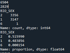
c1 = data['BIO_SEX'].value_counts(sort=False) print (c1)
p1 = data['BIO_SEX'].value_counts(sort=False, normalize=True) print (p1)
c2 = data['H1SU1'].value_counts(sort=False) print(c2)
p2 = data['H1SU1'].value_counts(sort=False, normalize=True) print (p2)
c3 = data['H1SU2'].value_counts(sort=False) print(c3)
p3 = data['H1SU2'].value_counts(sort=False, normalize=True) print (p3)
c4 = data['H1TO15'].value_counts(sort=False) print(c4)
ADDING TITLES
print ('counts for BIO_SEX') c1 = data['BIO_SEX'].value_counts(sort=False) print (c1)
print (len(data['BIO_SEX'])) #number of observations (rows)
print ('percentages for BIO_SEX') p1 = data['BIO_SEX'].value_counts(sort=False, normalize=True) print (p1)
print ('counts for H1SU1') c2 = data['H1SU1'].value_counts(sort=False) print(c2)
print ('percentages for H1SU1') p2 = data['H1SU1'].value_counts(sort=False, normalize=True) print (p2)
print ('counts for H1SU2') c3 = data['H1SU2'].value_counts(sort=False, dropna=False) print(c3)
print ('percentages for H1SU2') p3 = data['H1SU2'].value_counts(sort=False, normalize=True) print (p3)
print ('counts for H1TO15') c4 = data['H1TO15'].value_counts(sort=False, dropna=False) print(c4)
print ('percentages for H1TO15') p4 = data['H1TO15'].value_counts(sort=False, dropna=False, normalize=True) print (p4)
ADDING MORE DESCRIPTIVE TITLES
print('counts for BIO_SEX“ what is the gender') c1 = data['BIO_SEX'].value_counts(sort=False) print (c1)
print('percentages for BIO_SEX what is the gender') p1 = data['BIO_SEX'].value_counts(sort=False, normalize=True) print (p1)
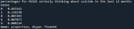
print('counts for H1SU1 seriosly thinking about suicide in the last 12 months') c2 = data['H1SU1'].value_counts(sort=False) print(c2)
print('percentages for H1SU1 seriosly thinking about suicide in the last 12 months') p2 = data['H1SU1'].value_counts(sort=False, normalize=True) print (p2)
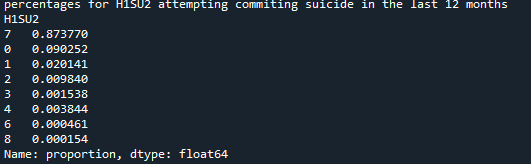
print('counts for H1SU2 attempting commiting suicide in the last 12 months') c3 = data['H1SU2'].value_counts(sort=False) print(c3)
print('percentages for H1SU2 attempting commiting suicide in the last 12 months') p3 = data['H1SU2'].value_counts(sort=False, normalize=True) print (p3)
print('counts for H1TO15 how many times a person thinks about alcohol during the past 12 months') c4 = data['H1TO15'].value_counts(sort=False, dropna=False) print(c4)
print('percentages for H1TO15 how many times a person thinks about alcohol during the past 12 months') p4 = data['H1TO15'].value_counts(sort=False, normalize=True) print (p4)
frequency distributions using the 'bygroup' function
ct1= data.groupby('BIO_SEX').size() print(ct1)
pt1 = data.groupby('BIO_SEX').size() * 100 / len(data) print(pt1)
subset data to male attempting commiting suicide in the last 12 months
sub1=data[(data['BIO_SEX']==1) & (data['H1SU1']==1)]
make a copy of my new subsetted data
sub2 = sub1.copy()
frequency distributions on new sub2 data frame
print('counts for BIO_SEX') c5 = sub2['BIO_SEX'].value_counts(sort=False) print(c5)
print('percentages for BIO_SEX') p5 = sub2['BIO_SEX'].value_counts(sort=False, normalize=True) print (p5)
print('counts for H1SU1') c6 = sub2['H1TO13'].value_counts(sort=False) print(c6)
print('percentages for H1SU1') p6 = sub2['H1SU1'].value_counts(sort=False, normalize=True) print (p6)
upper-case all DataFrame column names - place afer code for loading data aboave
data.columns = list(map(str.upper, data.columns))
bug fix for display formats to avoid run time errors - put after code for loading data above
pandas.set_option('display.float_format', lambda x:'%f'%x) Results: In this part we see how many male, how many female and undefined respondents there are, and what is that number expressed in percentages
Refining research question:
Research question is how many men seriously thought about committing suicide in the previous 12 months?


0 notes
Text
KMeans Clustering Assignment
Import the modules
from pandas import Series, DataFrame import pandas as pd import numpy as np import matplotlib.pylab as plt from sklearn.model_selection import train_test_split from sklearn import preprocessing from sklearn.cluster import KMeans
Load the dataset
data = pd.read_csv("C:\Users\guy3404\OneDrive - MDLZ\Documents\Cross Functional Learning\AI COP\Coursera\machine_learning_data_analysis\Datasets\tree_addhealth.csv")
data.head()
upper-case all DataFrame column names
data.columns = map(str.upper, data.columns)
Data Management
data_clean = data.dropna() data_clean.head()
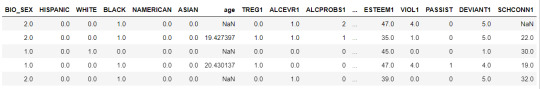
subset clustering variables
cluster=data_clean[['ALCEVR1','MAREVER1','ALCPROBS1','DEVIANT1','VIOL1', 'DEP1','ESTEEM1','SCHCONN1','PARACTV', 'PARPRES','FAMCONCT']] cluster.describe()

standardize clustering variables to have mean=0 and sd=1
clustervar=cluster.copy() clustervar['ALCEVR1']=preprocessing.scale(clustervar['ALCEVR1'].astype('float64')) clustervar['ALCPROBS1']=preprocessing.scale(clustervar['ALCPROBS1'].astype('float64')) clustervar['MAREVER1']=preprocessing.scale(clustervar['MAREVER1'].astype('float64')) clustervar['DEP1']=preprocessing.scale(clustervar['DEP1'].astype('float64')) clustervar['ESTEEM1']=preprocessing.scale(clustervar['ESTEEM1'].astype('float64')) clustervar['VIOL1']=preprocessing.scale(clustervar['VIOL1'].astype('float64')) clustervar['DEVIANT1']=preprocessing.scale(clustervar['DEVIANT1'].astype('float64')) clustervar['FAMCONCT']=preprocessing.scale(clustervar['FAMCONCT'].astype('float64')) clustervar['SCHCONN1']=preprocessing.scale(clustervar['SCHCONN1'].astype('float64')) clustervar['PARACTV']=preprocessing.scale(clustervar['PARACTV'].astype('float64')) clustervar['PARPRES']=preprocessing.scale(clustervar['PARPRES'].astype('float64'))
split data into train and test sets
clus_train, clus_test = train_test_split(clustervar, test_size=.3, random_state=123)
k-means cluster analysis for 1-9 clusters
from scipy.spatial.distance import cdist clusters=range(1,10) meandist=[]
for k in clusters: model=KMeans(n_clusters=k) model.fit(clus_train) clusassign=model.predict(clus_train) meandist.append(sum(np.min(cdist(clus_train, model.cluster_centers_, 'euclidean'), axis=1)) / clus_train.shape[0])
""" Plot average distance from observations from the cluster centroid to use the Elbow Method to identify number of clusters to choose """ plt.plot(clusters, meandist) plt.xlabel('Number of clusters') plt.ylabel('Average distance') plt.title('Selecting k with the Elbow Method')
Interpret 3 cluster solution
model3=KMeans(n_clusters=3) model3.fit(clus_train) clusassign=model3.predict(clus_train)
plot clusters
from sklearn.decomposition import PCA pca_2 = PCA(2) plot_columns = pca_2.fit_transform(clus_train) plt.scatter(x=plot_columns[:,0], y=plot_columns[:,1], c=model3.labels_,) plt.xlabel('Canonical variable 1') plt.ylabel('Canonical variable 2') plt.title('Scatterplot of Canonical Variables for 3 Clusters') plt.show()
The datapoints of the 2 clusters in the left are less spread out but have more overlaps. The cluster to the right is more distinct but has more spread in the data points
""" BEGIN multiple steps to merge cluster assignment with clustering variables to examine cluster variable means by cluster """
create a unique identifier variable from the index for the
cluster training data to merge with the cluster assignment variable
clus_train.reset_index(level=0, inplace=True)
create a list that has the new index variable
cluslist=list(clus_train['index'])
create a list of cluster assignments
labels=list(model3.labels_)
combine index variable list with cluster assignment list into a dictionary
newlist=dict(zip(cluslist, labels)) newlist
convert newlist dictionary to a dataframe
newclus=DataFrame.from_dict(newlist, orient='index') newclus
rename the cluster assignment column
newclus.columns = ['cluster']
now do the same for the cluster assignment variable
create a unique identifier variable from the index for the
cluster assignment dataframe
to merge with cluster training data
newclus.reset_index(level=0, inplace=True)
merge the cluster assignment dataframe with the cluster training variable dataframe
by the index variable
merged_train=pd.merge(clus_train, newclus, on='index') merged_train.head(n=100)
cluster frequencies
merged_train.cluster.value_counts()
""" END multiple steps to merge cluster assignment with clustering variables to examine cluster variable means by cluster """
FINALLY calculate clustering variable means by cluster
clustergrp = merged_train.groupby('cluster').mean() print ("Clustering variable means by cluster") print(clustergrp)
validate clusters in training data by examining cluster differences in GPA using ANOVA
first have to merge GPA with clustering variables and cluster assignment data
gpa_data=data_clean['GPA1']
split GPA data into train and test sets
gpa_train, gpa_test = train_test_split(gpa_data, test_size=.3, random_state=123) gpa_train1=pd.DataFrame(gpa_train) gpa_train1.reset_index(level=0, inplace=True) merged_train_all=pd.merge(gpa_train1, merged_train, on='index') sub1 = merged_train_all[['GPA1', 'cluster']].dropna()
Print statistical summary by cluster
import statsmodels.formula.api as smf import statsmodels.stats.multicomp as multi
gpamod = smf.ols(formula='GPA1 ~ C(cluster)', data=sub1).fit() print (gpamod.summary())
print ('means for GPA by cluster') m1= sub1.groupby('cluster').mean() print (m1)
print ('standard deviations for GPA by cluster') m2= sub1.groupby('cluster').std() print (m2)
Interpretation
The clustering average summary shows Cluster 0 has higher alcohol and marijuana problems, shows higher deviant and violent behavior, suffers from depression, has low self esteem,school connectedness, paraental and family connectedness. On the contrary, Cluster 2 shows the lowest alcohol and marijuana problems, lowest deviant & violent behavior,depression, and higher self esteem,school connectedness, paraental and family connectedness. Further, when validated against GPA score, we observe Cluster 0 shows the lowest average GPA and CLuster 2 has the highest average GPA which aligns with the summary statistics interpretation.
1 note
·
View note
Text
Program Data Analysis Tools: Module 4. Moderating variable
# -*- coding: utf-8 -*-
"""
Created on Fri Sep 8 11:25:51 2023
@author: ANA4MD
"""
# ANOVA
import numpy
import pandas
import statsmodels.formula.api as smf
import statsmodels.stats.multicomp as multi
import seaborn
import matplotlib.pyplot as plt
data = pandas.read_csv('gapminder.csv', low_memory=False)
# lower-case all DataFrame column names - place after code for loading data above
data.columns = list(map(str.lower, data.columns))
# bug fix for display formats to avoid run time errors - put after code for loading data above
pandas.set_option('display.float_format', lambda x: '%f' % x)
# to fix empty data to avoid errors
data = data.replace(r'^\s*$', numpy.NaN, regex=True)
# checking the format of my variables and set to numeric
data['femaleemployrate'].dtype
data['lifeexpectancy'].dtype
data['incomeperperson'].dtype
#data['urbanrate'].dtype
data['femaleemployrate'] = pandas.to_numeric(data['femaleemployrate'], errors='coerce', downcast=None)
data['lifeexpectancy'] = pandas.to_numeric(data['lifeexpectancy'], errors='coerce', downcast=None)
data['incomeperperson'] = pandas.to_numeric(data['incomeperperson'], errors='coerce', downcast=None)
#data['urbanrate'] = pandas.to_numeric(data['urbanrate'], errors='coerce', downcast=None)
#print('The explantory variable is the urban rate in 2 levels (rural, urban)')
#print('distribution for urban rate in 2 groups (rural, urban) and creating a new variable urban as categorical variable')
#data['urbanclass'] = pandas.cut(data['urbanrate'], [0, 20, 100], labels=['rural', 'urban'])
#c1 = data['urbanclass'].value_counts(sort=False, dropna=False)
#print (c1)
print('The explantory variable is the income per person in 3 levels (low class, midle class, upper class)')
print('distribution for income per person splits into 3 groups and creating a new variable income as categorical variable')
data['income'] = pandas.cut(data['incomeperperson'], [0, 2000, 24000, 120000], labels=['low class', 'middle class', 'upper class'])
c2 = data['income'].value_counts(sort=False, dropna=False)
print (c2)
print('The explantory variable is the life expectancy in 2 levels ( low, high)')
print('distribution for life expectancy in 2 groups (low, high) and creating a new variable urban as categorical variable')
data['life'] = pandas.cut(data['lifeexpectancy'], [0, 70, 100], labels=['low', 'high'])
c3 = data['life'].value_counts(sort=False, dropna=False)
print (c3)
model1 = smf.ols(formula='femaleemployrate ~ C(income)', data=data).fit()
print (model1.summary())
sub1 = data[['femaleemployrate', 'income']].dropna()
print ("means for femaleemployrate by income (low class, middle class, upper class)")
m1= sub1.groupby('income').mean()
print (m1)
print ("standard deviation for mean femaleemployrate by income (low class, middle class, upper class)")
st1= sub1.groupby('income').std()
print (st1)
# bivariate bar graph
seaborn.factorplot(x="income", y="femaleemployrate", data=data, kind="bar", ci=None)
plt.xlabel('income level')
plt.ylabel('Mean female employ %')
sub2=data[(data['life']=='low')]
sub3=data[(data['life']=='high')]
print ('association between income and femaleemploy rate for those with less life expectancy (Low)')
model2 = smf.ols(formula='femaleemployrate ~ C(income)', data=sub2).fit()
print (model2.summary())
print ("means for femaleemployrate by income (low class, middle class, upper class,) for low life expectancy")
m2= sub2.groupby('income').mean()
print (m2)
# bivariate bar graph
seaborn.factorplot(x="income", y="femaleemployrate", data=sub2, kind="bar", ci=None)
plt.xlabel('income level')
plt.ylabel('Mean female employ %')
print ('association between income and femaleemploy ratefor those with more life expectancy (high)')
model3 = smf.ols(formula='femaleemployrate ~ C(income)', data=sub3).fit()
print (model3.summary())
print ("means for femaleemployrate by income (low class, middle class, upper class) for high life expectancy")
m3 = sub3.groupby('income').mean()
print (m3)
# bivariate bar graph
seaborn.factorplot(x="income", y="femaleemployrate", data=sub3, kind="bar", ci=None)
plt.xlabel('income level')
plt.ylabel('Mean female employ %')
0 notes
Text
Lasso Regression
SCRIPT:
from pandas import Series, DataFrame import pandas as pd import numpy as np import os
from pandas import Series, DataFrame
import pandas as pd import numpy as np import matplotlib.pylab as plt from sklearn.model_selection import train_test_split from sklearn.linear_model import LassoLarsCV
Load the dataset
data = pd.read_csv("_358bd6a81b9045d95c894acf255c696a_nesarc_pds.csv") data=pd.DataFrame(data) data = data.replace(r'^\s*$', 101, regex=True)
upper-case all DataFrame column names
data.columns = map(str.upper, data.columns)
Data Management
data_clean = data.dropna()
select predictor variables and target variable as separate data sets
predvar= data_clean[['SEX','S1Q1E','S1Q7A9','S1Q7A10','S2AQ5A','S2AQ1','S2BQ1A20','S2CQ1','S2CQ2A10']]
target = data_clean.S2AQ5B
standardize predictors to have mean=0 and sd=1
predictors=predvar.copy() from sklearn import preprocessing predictors['SEX']=preprocessing.scale(predictors['SEX'].astype('float64')) predictors['S1Q1E']=preprocessing.scale(predictors['S1Q1E'].astype('float64')) predictors['S1Q7A9']=preprocessing.scale(predictors['S1Q7A9'].astype('float64')) predictors['S1Q7A10']=preprocessing.scale(predictors['S1Q7A10'].astype('float64')) predictors['S2AQ5A']=preprocessing.scale(predictors['S2AQ5A'].astype('float64')) predictors['S2AQ1']=preprocessing.scale(predictors['S2AQ1'].astype('float64')) predictors['S2BQ1A20']=preprocessing.scale(predictors['S2BQ1A20'].astype('float64')) predictors['S2CQ1']=preprocessing.scale(predictors['S2CQ1'].astype('float64')) predictors['S2CQ2A10']=preprocessing.scale(predictors['S2CQ2A10'].astype('float64'))
split data into train and test sets
pred_train, pred_test, tar_train, tar_test = train_test_split(predictors, target, test_size=.3, random_state=150)
specify the lasso regression model
model=LassoLarsCV(cv=10, precompute=False).fit(pred_train,tar_train)
print variable names and regression coefficients
dict(zip(predictors.columns, model.coef_))
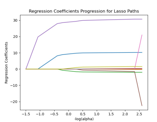
plot coefficient progression
m_log_alphas = -np.log10(model.alphas_) ax = plt.gca() plt.plot(m_log_alphas, model.coef_path_.T) plt.axvline(-np.log10(model.alpha_), linestyle='--', color='k', label='alpha CV') plt.ylabel('Regression Coefficients') plt.xlabel('-log(alpha)') plt.title('Regression Coefficients Progression for Lasso Paths')
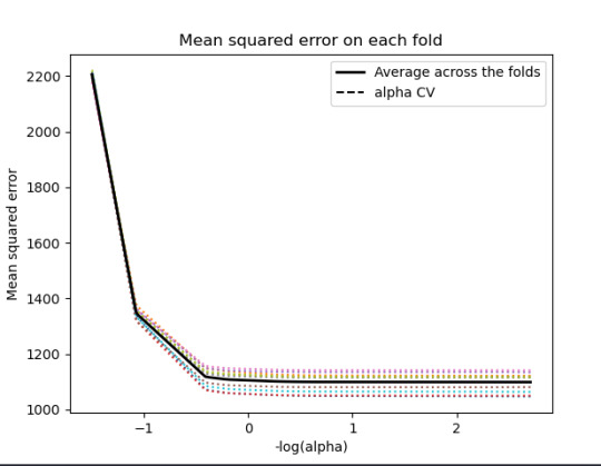
plot mean square error for each fold
m_log_alphascv = -np.log10(model.cv_alphas_) plt.figure() plt.plot(m_log_alphascv, model.mse_path_, ':') plt.plot(m_log_alphascv, model.mse_path_.mean(axis=-1), 'k', label='Average across the folds', linewidth=2) plt.axvline(-np.log10(model.alpha_), linestyle='--', color='k', label='alpha CV') plt.legend() plt.xlabel('-log(alpha)') plt.ylabel('Mean squared error') plt.title('Mean squared error on each fold')
MSE from training and test data
from sklearn.metrics import mean_squared_error train_error = mean_squared_error(tar_train, model.predict(pred_train)) test_error = mean_squared_error(tar_test, model.predict(pred_test)) print ('training data MSE') print(train_error) print ('test data MSE') print(test_error)
R-square from training and test data
rsquared_train=model.score(pred_train,tar_train) rsquared_test=model.score(pred_test,tar_test) print ('training data R-square') print(rsquared_train) print ('test data R-square') print(rsquared_test)
------------------------------------------------------------------------------
Graphs:
------------------------------------------------------------------------------
Analysing:
Output:
{'SEX': 10.217613940138108, 'S1Q1E': -0.31812083770240274, -ORIGIN OR DESCENT 'S1Q7A9': -1.9895640844032882, -PRESENT SITUATION INCLUDES RETIRED 'S1Q7A10': 0.30762235836398083, -PRESENT SITUATION INCLUDES IN SCHOOL FULL TIME 'S2AQ5A': 30.66524941440075, 'S2AQ1': -41.766164381325154, -DRANK AT LEAST 1 ALCOHOLIC DRINK IN LIFE 'S2BQ1A20': 73.94927622433774, - EVER HAVE JOB OR SCHOOL TROUBLES BECAUSE OF DRINKING 'S2CQ1': -33.74074926708572, -EVER SOUGHT HELP BECAUSE OF DRINKING 'S2CQ2A10': 1.6103002338271737} -EVER WENT TO EMPLOYEE ASSISTANCE PROGRAM (EAP)
training data MSE 1097.5883983117358 test data MSE 1098.0847471196266 training data R-square 0.50244242170729 test data R-square 0.4974333966086808
------------------------------------------------------------------------------
Conclusions:
I was looking at the questions, how often Brank beer in the last 12 Months?
We can see that the following variables are the most important variables to be able to answer the questions.
S2BQ1A20:EVER HAVE JOB OR SCHOOL TROUBLES BECAUSE OF DRINKING
S2AQ1:DRANK AT LEAST 1 ALCOHOLIC DRINK IN LIFE
S2CQ1:EVER SOUGHT HELP BECAUSE OF DRINKING
All the important variables are related to drinking. The Root squared for both the training and the test data is very small and very similar which means the training data set wasn't overfitted and not too biased.
30% was the training set and 70% was the test set, each set had 150 random states. The graph are showing 10 lasso regression coefficients
0 notes
Text
Linear regression alcohol consumption vs number of alcoholic parents
Code
import pandas import numpy import matplotlib.pyplot as plt from sklearn.linear_model import LinearRegression from sklearn.model_selection import train_test_split from sklearn.metrics import mean_squared_error, r2_score import statsmodels.api as sm import seaborn import statsmodels.formula.api as smf
print("start import") data = pandas.read_csv('nesarc_pds.csv', low_memory=False) print("import done")
upper-case all Dataframe column names --> unification
data.colums = map(str.upper, data.columns)
bug fix for display formats to avoid run time errors
pandas.set_option('display.float_format', lambda x:'%f'%x)
print (len(data)) #number of observations (rows) print (len(data.columns)) # number of variables (columns)
checking the format of your variables
setting variables you will be working with to numeric
data['S2DQ1'] = pandas.to_numeric(data['S2DQ1']) #Blood/Natural Father data['S2DQ2'] = pandas.to_numeric(data['S2DQ2']) #Blood/Natural Mother data['S2BQ3A'] = pandas.to_numeric(data['S2BQ3A'], errors='coerce') #Age at first Alcohol abuse data['S3CQ14A3'] = pandas.to_numeric(data['S3CQ14A3'], errors='coerce')
Blood/Natural Father was alcoholic
print("number blood/natural father was alcoholic")
0 = no; 1= yes; unknown = nan
data['S2DQ1'] = data['S2DQ1'].replace({2: 0, 9: numpy.nan}) c1 = data['S2DQ1'].value_counts(sort=False).sort_index() print (c1)
print("percentage blood/natural father was alcoholic") p1 = data['S2DQ1'].value_counts(sort=False, normalize=True).sort_index() print (p1)
Blood/Natural Mother was alcoholic
print("number blood/natural mother was alcoholic")
0 = no; 1= yes; unknown = nan
data['S2DQ2'] = data['S2DQ2'].replace({2: 0, 9: numpy.nan}) c2 = data['S2DQ2'].value_counts(sort=False).sort_index() print(c2)
print("percentage blood/natural mother was alcoholic") p2 = data['S2DQ2'].value_counts(sort=False, normalize=True).sort_index() print (p2)
Data Management: Number of parents with background of alcoholism is calculated
0 = no parents; 1 = at least 1 parent (maybe one answer missing); 2 = 2 parents; nan = 1 unknown and 1 zero or both unknown
print("number blood/natural parents was alcoholic") data['Num_alcoholic_parents'] = numpy.where((data['S2DQ1'] == 1) & (data['S2DQ2'] == 1), 2, numpy.where((data['S2DQ1'] == 1) & (data['S2DQ2'] == 0), 1, numpy.where((data['S2DQ1'] == 0) & (data['S2DQ2'].isna()), numpy.nan, numpy.where((data['S2DQ1'] == 0) & (data['S2DQ2'].isna()), numpy.nan, numpy.where((data['S2DQ1'] == 0) & (data['S2DQ2'] == 0), 0, numpy.nan)))))
c5 = data['Num_alcoholic_parents'].value_counts(sort=False).sort_index() print(c5)
print("percentage blood/natural parents was alcoholic") p5 = data['Num_alcoholic_parents'].value_counts(sort=False, normalize=True).sort_index() print (p5)
___________________________________________________________________Graphs_________________________________________________________________________
Diagramm für c5 erstellen
plt.figure(figsize=(8, 5)) plt.bar(c5.index, c5.values) plt.xlabel('Num_alcoholic_parents') plt.ylabel('Häufigkeit') plt.title('Häufigkeitsverteilung von Num_alcoholic_parents') plt.xticks(c5.index) plt.show()
Diagramm für p5 erstellen
plt.figure(figsize=(8, 5)) plt.bar(p5.index, p5.values*100) plt.xlabel('Num_alcoholic_parents') plt.ylabel('Häufigkeit (%)') plt.title('Häufigkeitsverteilung von Num_alcoholic_parents') plt.xticks(c5.index) plt.show()
print("lineare Regression")
Entfernen Sie Zeilen mit NaN-Werten in den relevanten Spalten.
data_cleaned = data.dropna(subset=['Num_alcoholic_parents', 'S2BQ3A'])
Definieren Sie Ihre unabhängige Variable (X) und Ihre abhängige Variable (y).
X = data_cleaned['Num_alcoholic_parents'] y = data_cleaned['S2BQ3A']
Fügen Sie eine Konstante hinzu, um den Intercept zu berechnen.
X = sm.add_constant(X)
Erstellen Sie das lineare Regressionsmodell.
model = sm.OLS(y, X).fit()
Drucken Sie die Zusammenfassung des Modells.
print(model.summary()) Result
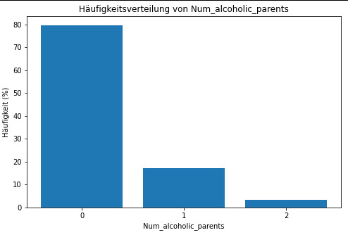
frequency distribution shows how many of the people from the study have alcoholic parents and if its only 1 oder both parents.
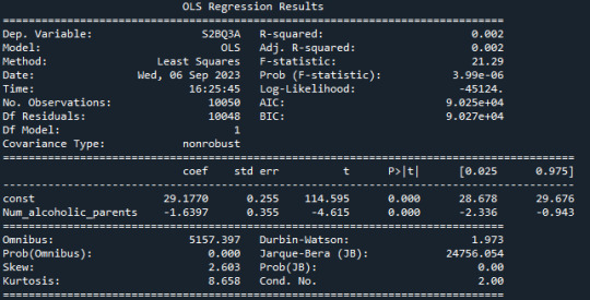
R-squared: The R-squared value is 0.002, indicating that only about 0.2% of the variation in "S2BQ3A" (quantity of alcoholic drinks consumed) is explained by the variable "Num_alcoholic_parents" (number of alcoholic parents). This suggests that there is likely no strong linear relationship between these two variables.
F-statistic: The F-statistic has a value of 21.29, and the associated probability (Prob (F-statistic)) is very small (3.99e-06). The F-statistic is used to assess the overall effectiveness of the model. In this case, the low probability suggests that at least one of the independent variables has a significant impact on the dependent variable.
Coefficients: The coefficients of the model show the estimated effects of the independent variables on the dependent variable. In this case, the constant (const) has a value of 29.1770, representing the estimated average value of "S2BQ3A" when "Num_alcoholic_parents" is zero. The coefficient for "Num_alcoholic_parents" is -1.6397, meaning that an additional alcoholic parent is associated with an average decrease of 1.6397 units in "S2BQ3A" (quantity of alcoholic drinks consumed).
P-Values (P>|t|): The p-values next to the coefficients indicate the significance of each coefficient. In this case, both the constant and the coefficient for "Num_alcoholic_parents" are highly significant (p-values close to zero). This suggests that "Num_alcoholic_parents" has a statistically significant impact on "S2BQ3A."
AIC and BIC: AIC (Akaike Information Criterion) and BIC (Bayesian Information Criterion) are model evaluation measures. Lower values indicate a better model fit. In this case, both AIC and BIC are relatively low, which could indicate the adequacy of the model.
In summary, there is a statistically significant but very weak negative relationship between the number of alcoholic parents and the quantity of alcoholic drinks consumed. This means that an increase in the number of alcoholic parents is associated with a slight decrease in the quantity of alcohol consumed, but it explains only a very limited amount of the variation in the quantity of alcohol consumed.
0 notes
Text
rom pandas import Series, DataFrame import pandas as pd import numpy as np import matplotlib.pylab as plt from sklearn.model_selection import train_test_split from sklearn import preprocessing from sklearn.cluster import KMeans
""" Data Management """ data = pd.read_csv("tree_addhealth")
upper-case all DataFrame column names
data.columns = map(str.upper, data.columns)
Data Management
data_clean = data.dropna()
subset clustering variables
cluster=data_clean[['ALCEVR1','MAREVER1','ALCPROBS1','DEVIANT1','VIOL1', 'DEP1','ESTEEM1','SCHCONN1','PARACTV', 'PARPRES','FAMCONCT']] cluster.describe()
standardize clustering variables to have mean=0 and sd=1
clustervar=cluster.copy() clustervar['ALCEVR1']=preprocessing.scale(clustervar['ALCEVR1'].astype('float64')) clustervar['ALCPROBS1']=preprocessing.scale(clustervar['ALCPROBS1'].astype('float64')) clustervar['MAREVER1']=preprocessing.scale(clustervar['MAREVER1'].astype('float64')) clustervar['DEP1']=preprocessing.scale(clustervar['DEP1'].astype('float64')) clustervar['ESTEEM1']=preprocessing.scale(clustervar['ESTEEM1'].astype('float64')) clustervar['VIOL1']=preprocessing.scale(clustervar['VIOL1'].astype('float64')) clustervar['DEVIANT1']=preprocessing.scale(clustervar['DEVIANT1'].astype('float64')) clustervar['FAMCONCT']=preprocessing.scale(clustervar['FAMCONCT'].astype('float64')) clustervar['SCHCONN1']=preprocessing.scale(clustervar['SCHCONN1'].astype('float64')) clustervar['PARACTV']=preprocessing.scale(clustervar['PARACTV'].astype('float64')) clustervar['PARPRES']=preprocessing.scale(clustervar['PARPRES'].astype('float64'))
split data into train and test sets
clus_train, clus_test = train_test_split(clustervar, test_size=.3, random_state=123)
k-means cluster analysis for 1-9 clusters
from scipy.spatial.distance import cdist clusters=range(1,10) meandist=[]
for k in clusters: model=KMeans(n_clusters=k) model.fit(clus_train) clusassign=model.predict(clus_train) meandist.append(sum(np.min(cdist(clus_train, model.cluster_centers_, 'euclidean'), axis=1)) / clus_train.shape[0])
""" Plot average distance from observations from the cluster centroid to use the Elbow Method to identify number of clusters to choose """
plt.plot(clusters, meandist) plt.xlabel('Number of clusters') plt.ylabel('Average distance') plt.title('Selecting k with the Elbow Method')
Interpret 3 cluster solution
model3=KMeans(n_clusters=3) model3.fit(clus_train) clusassign=model3.predict(clus_train)
plot clusters
from sklearn.decomposition import PCA pca_2 = PCA(2) plot_columns = pca_2.fit_transform(clus_train) plt.scatter(x=plot_columns[:,0], y=plot_columns[:,1], c=model3.labels_,) plt.xlabel('Canonical variable 1') plt.ylabel('Canonical variable 2') plt.title('Scatterplot of Canonical Variables for 3 Clusters') plt.show()
""" BEGIN multiple steps to merge cluster assignment with clustering variables to examine cluster variable means by cluster """
create a unique identifier variable from the index for the
cluster training data to merge with the cluster assignment variable
clus_train.reset_index(level=0, inplace=True)
create a list that has the new index variable
cluslist=list(clus_train['index'])
create a list of cluster assignments
labels=list(model3.labels_)
combine index variable list with cluster assignment list into a dictionary
newlist=dict(zip(cluslist, labels)) newlist
convert newlist dictionary to a dataframe
newclus=DataFrame.from_dict(newlist, orient='index') newclus
rename the cluster assignment column
newclus.columns = ['cluster']
now do the same for the cluster assignment variable
create a unique identifier variable from the index for the
cluster assignment dataframe
to merge with cluster training data
newclus.reset_index(level=0, inplace=True)
merge the cluster assignment dataframe with the cluster training variable dataframe
by the index variable
merged_train=pd.merge(clus_train, newclus, on='index') merged_train.head(n=100)
cluster frequencies
merged_train.cluster.value_counts()
""" END multiple steps to merge cluster assignment with clustering variables to examine cluster variable means by cluster """
FINALLY calculate clustering variable means by cluster
clustergrp = merged_train.groupby('cluster').mean() print ("Clustering variable means by cluster") print(clustergrp)
validate clusters in training data by examining cluster differences in GPA using ANOVA
first have to merge GPA with clustering variables and cluster assignment data
gpa_data=data_clean['GPA1']
split GPA data into train and test sets
gpa_train, gpa_test = train_test_split(gpa_data, test_size=.3, random_state=123) gpa_train1=pd.DataFrame(gpa_train) gpa_train1.reset_index(level=0, inplace=True) merged_train_all=pd.merge(gpa_train1, merged_train, on='index') sub1 = merged_train_all[['GPA1', 'cluster']].dropna()
import statsmodels.formula.api as smf import statsmodels.stats.multicomp as multi
gpamod = smf.ols(formula='GPA1 ~ C(cluster)', data=sub1).fit() print (gpamod.summary())
print ('means for GPA by cluster') m1= sub1.groupby('cluster').mean() print (m1)
print ('standard deviations for GPA by cluster') m2= sub1.groupby('cluster').std() print (m2)
mc1 = multi.MultiComparison(sub1['GPA1'], sub1['cluster']) res1 = mc1.tukeyhsd() print(res1.summary())
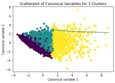
0 notes
Text
Código K- means craters of mars
-- coding: utf-8 --
""" Created on Fri Jun 16 19:08:39 2023
@author: ANGELA """ from pandas import Series, DataFrame import pandas import numpy as np import matplotlib.pylab as plt from sklearn.model_selection import train_test_split from sklearn import preprocessing from sklearn.cluster import KMeans
"""Data management"""
data = pandas.read_csv('marscrater_pds.csv', low_memory=False) data['LATITUDE_CIRCLE_IMAGE']=pandas.to_numeric(data['LATITUDE_CIRCLE_IMAGE'],errors='coerce') data['LONGITUDE_CIRCLE_IMAGE']=pandas.to_numeric(data['LONGITUDE_CIRCLE_IMAGE'],errors='coerce') data['DIAM_CIRCLE_IMAGE']=pandas.to_numeric(data['DIAM_CIRCLE_IMAGE'],errors='coerce') data['NUMBER_LAYERS']=pandas.to_numeric(data['NUMBER_LAYERS'],errors='coerce') data['DEPTH_RIMFLOOR_TOPOG']=pandas.to_numeric(data['DEPTH_RIMFLOOR_TOPOG'],errors='coerce')
upper-case all DataFrame column names
data.columns = map(str.upper, data.columns) data_clean =data.dropna()
target = data_clean.DEPTH_RIMFLOOR_TOPOG
select predictor variables and target variable as separate data sets
cluster= data_clean[['LATITUDE_CIRCLE_IMAGE','LONGITUDE_CIRCLE_IMAGE','DIAM_CIRCLE_IMAGE']] cluster.describe()
standardize clustering variables to have mean=0 and sd=1
clustervar=cluster.copy() clustervar['LATITUDE_CIRCLE_IMAGE']=preprocessing.scale(clustervar['LATITUDE_CIRCLE_IMAGE'].astype('float64')) clustervar['LONGITUDE_CIRCLE_IMAGE']=preprocessing.scale(clustervar['LONGITUDE_CIRCLE_IMAGE'].astype('float64')) clustervar['DIAM_CIRCLE_IMAGE']=preprocessing.scale(clustervar['DIAM_CIRCLE_IMAGE'].astype('float64'))
clustervar['DEPTH_RIMFLOOR_TOPOG']=preprocessing.scale(clustervar['DEPTH_RIMFLOOR_TOPOG'].astype('float64'))
split data into train and test sets
clus_train, clus_test = train_test_split(clustervar, test_size=.3, random_state=200)
k-means cluster analysis for 1-9 clusters
from scipy.spatial.distance import cdist clusters=range(1,10) meandist=[]
Calculate cluster
for k in clusters: model=KMeans(n_clusters=k) model.fit(clus_train) clusassign=model.predict(clus_train) meandist.append(sum(np.min(cdist(clus_train, model.cluster_centers_, 'euclidean'), axis=1)) / clus_train.shape[0])
""" Plot average distance from observations from the cluster centroid to use the Elbow Method to identify number of clusters to choose """
plt.plot(clusters, meandist) plt.xlabel('Number of clusters') plt.ylabel('Average distance') plt.title('Selecting k with the Elbow Method to date craters of mars')
Interpret 3 cluster solution
model3=KMeans(n_clusters=3) model3.fit(clus_train) clusassign=model3.predict(clus_train)
plot clusters
from sklearn.decomposition import PCA pca_2 = PCA(2) plot_columns = pca_2.fit_transform(clus_train) plt.scatter(x=plot_columns[:,0], y=plot_columns[:,1], c=model3.labels_,) plt.xlabel('Canonical variable 1') plt.ylabel('Canonical variable 2') plt.title('Scatterplot of Canonical Variables for 3 Clusters to date craters of mars') plt.show()
""" BEGIN multiple steps to merge cluster assignment with clustering variables to examine cluster variable means by cluster """
create a unique identifier variable from the index for the
cluster training data to merge with the cluster assignment variable
clus_train.reset_index(level=0, inplace=True)
create a list that has the new index variable
cluslist=list(clus_train['index'])
create a list of cluster assignments
labels=list(model3.labels_)
combine index variable list with cluster assignment list into a dictionary
newlist=dict(zip(cluslist, labels)) newlist
convert newlist dictionary to a dataframe
newclus=DataFrame.from_dict(newlist, orient='index') newclus
rename the cluster assignment column
newclus.columns = ['cluster']
now do the same for the cluster assignment variable
create a unique identifier variable from the index for the
cluster assignment dataframe
to merge with cluster training data
newclus.reset_index(level=0, inplace=True)
merge the cluster assignment dataframe with the cluster training variable dataframe
by the index variable
merged_train=pandas.merge(clus_train, newclus, on='index') merged_train.head(n=100)
cluster frequencies
merged_train.cluster.value_counts()
""" END multiple steps to merge cluster assignment with clustering variables to examine cluster variable means by cluster """
FINALLY calculate clustering variable means by cluster
clustergrp = merged_train.groupby('cluster').mean() print ("Clustering variable means by cluster") print(clustergrp)
validate clusters in training data by examining cluster differences in DEPTH_RIMFLOOR_TOPOG using ANOVA
first have to merge DEPTH_RIMFLOOR_TOPOG with clustering variables and cluster assignment data
DRT_data=data_clean['DEPTH_RIMFLOOR_TOPOG']
split DEPTH_RIMFLOOR_TOPOG data into train and test sets
DRT_train, DRT_test = train_test_split(DRT_data, test_size=.3, random_state=123) DRT_train1=pandas.DataFrame(DRT_train) DRT_train1.reset_index(level=0, inplace=True) merged_train_all=pandas.merge(DRT_train1, merged_train, on='index') sub1 = merged_train_all[['DEPTH_RIMFLOOR_TOPOG', 'cluster']].dropna()
import statsmodels.formula.api as smf import statsmodels.stats.multicomp as multi
DTRmod = smf.ols(formula='DEPTH_RIMFLOOR_TOPOG ~ C(cluster)', data=sub1).fit() print (DTRmod.summary())
print ('means for DEPTH_RIMFLOOR_TOPOG by cluster') m1= sub1.groupby('cluster').mean() print (m1)
print ('standard deviations for DEPTH_RIMFLOOR_TOPOG by cluster') m2= sub1.groupby('cluster').std() print (m2)
mc1 = multi.MultiComparison(sub1['GPA1'], sub1['cluster']) res1 = mc1.tukeyhsd() print(res1.summary())
Resultados
Los cluster posibles son 3, 5, 7 y 8 donde se evidencia un punto de quiebre en la ilustración, por lo que se realizó la prueba con 3 clusters y se evidencia que puede presentarse un overfiting al esta muy cerca y cobre puestos los clusters
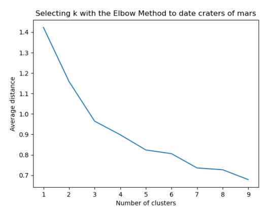
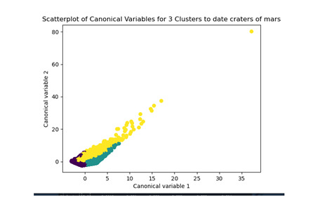
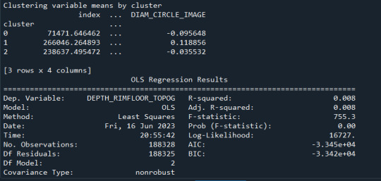

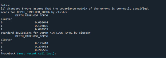
0 notes