#Cluster sampling vs other methods

[marketxcel]

Cluster Sampling: Types, Advantages, Limitations, and Examples

Explore the various types, advantages, limitations, and real-world examples of cluster sampling in our informative blog. Learn how this sampling method can help researchers gather data efficiently and effectively for insightful analysis.

[govindhtech]

Intel Extension For Scikit-learn: Time Series PCA & DBSCAN

Intel studies time series data clustering using density-based spatial clustering of applications with noise (DBSCAN) and PCA for dimensionality reduction. This approach detects patterns in time series data like city traffic flow without labelling. Intel Extension for Scikit-learn boosts performance. Machinery, human behaviour, and other quantitative elements often produce time series data patterns. Manually identifying these patterns is tough. PCA and DBSCAN are unsupervised learning methods that discover these patterns.

Data Creation

It generates synthetic waveform data for time series replication. Data consists of three waveforms supplemented with noise to simulate real-world unpredictability. The authors utilise Gaël Varoquaux's scikit-learn agglomerative clustering example. You may buy it under CC0 or BSD-3Clause.

Intel Extension for Scikit-learn speeds PCA and DBSCAN

PCA and DBSCAN may be accelerated with Intel Extension for Scikit-learn patching. Python module Scikit-learn does machine learning. The Intel Extension for Scikit-learn accelerates scikit-learn applications on Intel CPUs and GPUs in single- and multi-node setups. This plugin dynamically adjusts scikit-learn estimators to improve machine learning training and inference by 100x with equivalent mathematical soundness.

The Intel Extension for Scikit-learn uses the API, which may be activated via the command line or by modifying a few lines in your Python application before importing it:

To use patch_sklearn, import it from sklearnex.

Reduce Dimensionality using PCA

Intel uses PCA to reduce dimensionality and retain 99% of the dataset's variance before clustering 90 samples with 2,000 features:

It uses a pairplot to locate clusters in condensed data:

pd import pandas import seaborn sns

df = pd.DataFrame(XPC, columns=[‘PC1’, ‘PC2’, ‘PC3’, ‘PC4’]) sns.pairplot(df) plt.show()

A DBSCAN cluster

Intel chooses PC1 and PC2 for DBSCAN clustering because the pairplot splits the clusters. Also offered is a DBSCAN EPS parameter estimation. It chose 50 because the PC1 vs PC0 image suggests that the observed clusters should be separated by 50:

Clustered data may be plotted to assess DBSCAN's cluster detection.

Compared to Ground Truth

The graphic shows how effectively DBSCAN matches ground truth data and finds credible coloured groupings. Clustering recovered the data's patterns in this case. It effectively finds and categorises time series patterns using DBSCAN for clustering and PCA for dimensionality reduction. This approach allows data structure recognition without labelled samples.

Intel Scikit-learn Extension

Speed up scikit-learn for data analytics and ML

Python machine learning module scikit-learn is also known as sklearn. For Intel CPUs and GPUs, the Intel Extension for Scikit-learn seamlessly speeds single- and multi-node applications. This extension package dynamically patches scikit-learn estimators to improve machine learning methods.

The AI Tools plugin lets you use machine learning with AI packages.

This scikit-learn plugin lets you:

Increase inference and training 100-fold while retaining mathematical accuracy.

Continue using open-source scikit-learn API.

Enable and disable the extension with a few lines of code or the command line.

AI and machine learning development tools from Intel include scikit-learn and the Intel Extension for Scikit-learn.

Features

Replace present estimators with mathematically comparable accelerated ones to speed up scikit-learn (sklearn). Algorithm Supported

The Intel oneAPI Data Analytics Library (oneDAL) powers the accelerations, so you may run it on any x86 or Intel GPU.

Decide acceleration application:

Patch any compatible algorithm from the command line without changing code.

Two lines of Python code patch all compatible algorithms.

Your script should fix just specified algorithms.

Apply global patches and unpatches to all scikit-learn apps.

[mitcenter]

Descriptive vs Inferential Statistics: What Sets Them Apart?

Statistics is a critical field in data science and research, offering tools and methodologies for understanding data. Two primary branches of statistics are descriptive and inferential statistics, each serving unique purposes in data analysis. Understanding the differences between these two branches "descriptive vs inferential statistics" is essential for accurately interpreting and presenting data.

Descriptive Statistics: Summarizing Data

Descriptive statistics focuses on summarizing and describing the features of a dataset. This branch of statistics provides a way to present data in a manageable and informative manner, making it easier to understand and interpret.

Measures of Central Tendency: Descriptive statistics include measures like the mean (average), median (middle value), and mode (most frequent value), which provide insights into the central point around which data values cluster.

Measures of Dispersion: It also includes measures of variability or dispersion, such as the range, variance, and standard deviation. These metrics indicate the spread or dispersion of data points in a dataset, helping to understand the consistency or variability of the data.

Data Visualization: Descriptive statistics often utilize graphical representations like histograms, bar charts, pie charts, and box plots to visually summarize data. These visual tools can reveal patterns, trends, and distributions that might not be apparent from numerical summaries alone.

The primary goal of descriptive statistics is to provide a clear and concise summary of the data at hand. It does not, however, make predictions or infer conclusions beyond the dataset itself.

Inferential Statistics: Making Predictions and Generalizations

While descriptive statistics focus on summarizing data, inferential statistics go a step further by making predictions and generalizations about a population based on a sample of data. This branch of statistics is essential when it is impractical or impossible to collect data from an entire population.

Sampling and Estimation: Inferential statistics rely heavily on sampling techniques. A sample is a subset of a population, selected in a way that it represents the entire population. Estimation methods, such as point estimation and interval estimation, are used to infer population parameters (like the population mean or proportion) based on sample data.

Hypothesis Testing: This is a key component of inferential statistics. It involves making a claim or hypothesis about a population parameter and then using sample data to test the validity of that claim. Common tests include t-tests, chi-square tests, and ANOVA. The results of these tests help determine whether there is enough evidence to support or reject the hypothesis.

Confidence Intervals: Inferential statistics also involve calculating confidence intervals, which provide a range of values within which a population parameter is likely to lie. This range, along with a confidence level (usually 95% or 99%), indicates the degree of uncertainty associated with the estimate.

Regression Analysis and Correlation: These techniques are used to explore relationships between variables and make predictions. For example, regression analysis can help predict the value of a dependent variable based on one or more independent variables.

Key Differences and Applications

The primary difference between descriptive and inferential statistics lies in their objectives. Descriptive statistics aim to describe and summarize the data, providing a snapshot of the dataset's characteristics. Inferential statistics, on the other hand, aim to make inferences and predictions about a larger population based on a sample of data.

In practice, descriptive statistics are often used in the initial stages of data analysis to get a sense of the data's structure and key features. Inferential statistics come into play when researchers or analysts want to draw conclusions that extend beyond the immediate dataset, such as predicting trends, making decisions, or testing hypotheses.

In conclusion, both descriptive and inferential statistics are crucial for data analysis and statistical analysis, each serving distinct roles. Descriptive statistics provide the foundation by summarizing data, while inferential statistics allow for broader generalizations and predictions. Together, they offer a comprehensive toolkit for understanding and making decisions based on data.

[emergingindiaanalyticsnoida]

Statistical Foundations for Data Scientists: Key Concepts and Techniques

Introduction to Data Science and its Importance in the Digital Age

Welcome to the exciting world of data science, where numbers come alive and reveal hidden insights! In today’s digital age, data is king, and those who can harness its power hold the key to unlocking endless possibilities. But behind every successful data scientist lies a strong foundation in statistics. So buckle up as we dive deep into the statistical foundations that are essential for every aspiring data scientist to master!

Understanding the Role of Statistics in Data Science

In the realm of Data Science, statistics plays a crucial role in extracting meaningful insights from vast amounts of data.

Statistics provides the tools and techniques necessary to analyze data, uncover patterns, and make informed decisions based on evidence rather than intuition alone.

By utilizing statistical methods, Data Scientists can quantify uncertainty, identify trends, and test hypotheses to draw reliable conclusions about the phenomena they are studying.

From descriptive statistics that summarize key features of a dataset to inferential statistics that help generalize findings beyond the sample at hand, statisticians provide the foundation for sound data analysis.

Understanding statistical concepts like probability distributions, hypothesis testing, and regression analysis is essential for any Data Scientist looking to derive actionable insights from complex datasets.

Key Statistical Concepts for Data Scientists

When diving into the world of data science, understanding key statistical concepts is crucial. One fundamental concept is the distinction between descriptive and inferential statistics. Descriptive statistics help us summarize and describe data, while inferential statistics enable us to make predictions or inferences based on sample data.

Measures of central tendency such as mean, median, and mode provide insights into where the center of a dataset lies. Variability and standard deviation allow us to understand how spread out our data points are from the mean. These concepts are essential for interpreting and analyzing datasets effectively.

By grasping these key statistical concepts, data scientists can uncover patterns, trends, and relationships within their data. This knowledge forms the foundation for more advanced statistical techniques like hypothesis testing, regression analysis, and clustering — all valuable tools in extracting meaningful insights from complex datasets.

A. Descriptive vs Inferential Statistics

When diving into the world of data science, understanding the difference between descriptive and inferential statistics is fundamental. Descriptive statistics focus on summarizing and describing data through measures like mean, median, and mode. It provides insights into what the data is telling us at a specific point in time.

On the other hand, inferential statistics help make predictions or generalizations about a population based on sample data. It involves hypothesis testing to draw conclusions beyond the immediate data set. This branch of statistics allows us to infer trends or patterns that can be applied to larger datasets.

While descriptive statistics paint a clear picture of what has happened in the past, inferential statistics take it a step further by helping us understand what could happen in the future based on our current findings. Both play crucial roles in extracting valuable insights from data sets for decision-making processes.

B. Measures of Central Tendency

Measures of central tendency play a crucial role in summarizing data by identifying the center or average value. One commonly used measure is the mean, which calculates the arithmetic average of a dataset. It provides a single value that represents the entire set of observations.

Another essential measure is the median, which identifies the middle value when data points are arranged in ascending or descending order. Unlike the mean, it is not affected by extreme values, making it robust for skewed datasets.

The mode is yet another important measure that signifies the most frequently occurring value in a dataset. It can be particularly useful when analyzing categorical variables or identifying common patterns within data.

Each of these measures offers unique insights into the distribution and characteristics of data, helping data scientists make informed decisions based on central tendencies observed within their datasets.

C. Variability and Standard Deviation

Variability and standard deviation are crucial statistical concepts that data scientists rely on to understand the spread of data points in a dataset. Think of variability as the diversity or range within your data, showing how much individual values differ from the mean. Standard deviation quantifies this dispersion by calculating the average distance of each data point from the mean.

Data with high variability will have a larger standard deviation, indicating more significant differences between values. On the other hand, low variability results in a smaller standard deviation, meaning data points are closer to the mean. When analyzing datasets, understanding variability and standard deviation helps identify patterns, outliers, and trends that can guide decision-making processes.

By grasping these concepts effectively, data scientists can draw meaningful insights from their analyses and make informed recommendations based on robust statistical foundations.

Common Statistical Techniques used in Data Science

Statistical techniques play a crucial role in the field of data science by providing the tools needed to analyze and make sense of complex datasets. One common technique used is hypothesis testing, which allows data scientists to determine if there is a significant difference between groups or variables based on sample data. Regression analysis is another powerful statistical method that helps in understanding the relationships between variables and making predictions based on historical data.

Clustering is yet another essential technique where data points are grouped together based on similarities, enabling patterns and insights to emerge from large datasets. By applying these statistical methods, data scientists can uncover hidden trends, relationships, and patterns within their data, leading to valuable insights for decision-making processes.

A. Hypothesis Testing

Hypothesis testing is a vital statistical technique in the toolkit of data scientists. It allows us to make informed decisions based on data analysis rather than gut feelings or assumptions.

In hypothesis testing, we start by formulating a null hypothesis, assuming there is no significant difference between groups or variables. Then, we collect and analyze data to either reject or fail to reject this null hypothesis.

By setting up hypotheses and conducting tests with statistical significance levels, we can determine if our findings are due to chance or if they represent true relationships in the data.

This method helps us draw reliable conclusions from our datasets and provides a solid foundation for making evidence-based decisions in various industries like healthcare, finance, marketing, and beyond.

B. Regression Analysis

Regression Analysis is a powerful statistical technique that data scientists use to understand the relationship between variables. It helps predict the value of one variable based on the values of others. Imagine you want to forecast sales based on advertising spending; regression analysis can provide insights into this relationship.

There are different types of regression models, such as linear regression and logistic regression, each suited for specific scenarios. Linear regression predicts continuous outcomes, while logistic regression is used for binary outcomes like whether a customer will purchase a product or not.

By analyzing data patterns through regression analysis, data scientists can make informed decisions and develop predictive models. This method allows them to uncover trends, identify correlations, and ultimately derive valuable insights from complex datasets.

In essence, Regression Analysis plays a crucial role in the toolkit of every data scientist striving to extract meaningful information from vast amounts of data.

C. Clustering

Clustering is a powerful statistical technique that data scientists use to group similar data points together based on certain characteristics. By identifying patterns and relationships within datasets, clustering helps uncover hidden insights and trends that may not be apparent at first glance.

Through clustering algorithms like K-means or hierarchical clustering, data scientists can segment complex data into distinct clusters, enabling them to make more informed decisions and predictions. This technique is widely used in various industries such as marketing, healthcare, and finance to classify customers, patients, or financial transactions.

By applying clustering in real-world scenarios, businesses can optimize their marketing strategies by targeting specific customer segments with personalized campaigns. In healthcare, clustering helps identify patient groups with similar medical conditions for tailored treatment plans. Clustering plays a crucial role in extracting valuable information from large datasets and driving strategic decision-making processes.

How to Apply Statistical Methods in Real

As a data scientist, understanding statistical foundations is crucial for making informed decisions in the digital age. By grasping key concepts like descriptive versus inferential statistics, measures of central tendency, and variability, you can extract valuable insights from data.

Moreover, common statistical techniques such as hypothesis testing, regression analysis, and clustering play a vital role in uncovering patterns and relationships within datasets. By applying these methods effectively, data scientists can drive decision-making processes and enhance business strategies.

In real-world scenarios, statistical methods empower data scientists to analyze customer behavior trends, predict market outcomes, optimize resource allocation, and much more. Through the application of statistical techniques in practical settings, professionals can leverage the power of data to drive innovation and achieve tangible results.

Mastering statistical foundations equips data scientists with the tools needed to navigate complex datasets efficiently and extract meaningful insights that drive success in today’s data-driven world.

[drew-mga2022mi6021]

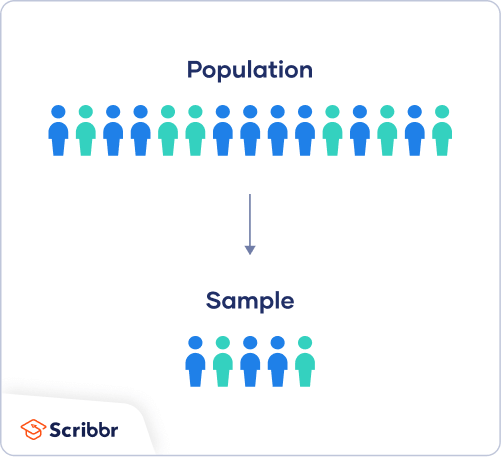
Research | Population vs Sample and Sample Strategies

via Scribbr

Within the context of research, a population is the entire group a researcher would want to draw conclusions on, whilst a sample is the group from which the data would be gathered to represent the population. The population can be defined based on a variety of factors, such as geographical location, age, income, etc. It can be very broad, or extremely specific based on the topic of research. Sampling itself can be divided into two sections;

Probability Sampling : A random selection of the population, allowing for strong statistical inferences about a given group.

Non-Probability Sampling : A Non random selection based on convenience or a certain criterion or criteria, allowing for easy collection of data.

Probability Sampling Methods

Probability Sampling is mainly used in quantitative research. It means that every member of the population has a chance of being selected. If the goal is to produce results representative of the whole population, probability sampling techniques are the most valid choice. These can be divided into four groups;

Simple Random Sample

Systematic Sample

Stratified Sample

Cluster Sample

The first technique dictates that any random member of the population has an equal chance of being selected. Therefore the sampling frame should include the whole population. To conduct this, RNG or other chance based techniques could be used to gather a sample. Systematic sampling is similar to simple random sampling, but it is usually slightly easier to conduct. Every member of the population is listed with a number, but instead of randomly generating numbers, individuals are chosen at regular intervals. It is important to make sure that there is no hidden pattern in the list that might skew the sample.

Stratified sampling involves dividing the population into subpopulations that may differ in important ways. It allows you draw more precise conclusions by ensuring that every subgroup is properly represented in the sample. This method involves separating the population into substrata based on characteristics such as age, gender, or other relevant factors. Based on the overall proportions of the population, the sample must be reflective of that ratio. So, the sample is formed by calculating the the number of people based on the size of the strata. After this, any of the above two sampling strategies could be used.

Cluster sampling also involves dividing the population into subgroups, but each subgroup should have similar characteristics to the whole sample. Instead of sampling individuals from each subgroup, you randomly select entire subgroups. While this method is better suited to dealing with large, dispersed populations, there is room for more error within the sample, as there could be substantial differences between clusters.

Non-Probability Sampling Methods

This sampling technique is based on non-random criteria, and not every individual has a chance to be included in the sample. This type of sampling is cheaper and easier to access, but runs a larger risk of sampling bias. If a non-probability sample is used, it must be as representative of the population as possible.

Non-probability sampling techniques are often used in qualitative research. The aim is not to test a hypothesis about a broad population, but to develop an initial understanding of a small or under-researched population. This too, can be divided into four groups;

Convenience Sample

Purposive Sample

Snowball Sample

Quota Sample

Convenience sampling is the most self-explanatory; it includes a population that is most accessible to the researcher. While it is easier, there is no way to guarantee generalisable results. Another method of sampling similar to this is voluntary response sampling, which involves voluntary action to help the researcher (eg;- an online survey). Alas, this method of selection is also somewhat biased, as some people are inherently more likely to volunteer than others, and thus are likely to have stronger opinions on a given topic.

Purposive sampling involves selecting a demography that is most useful towards the topic of research being conducted. It is often used in qualitative research, where the researcher wants to gain detailed knowledge about a specific phenomenon rather than make statistical inferences, or where the population is very small and specific. When using this method, a strong rationale and criteria need to be made clear based on inclusion and exclusion.

If a population is harder to access, a snowball sample can be used to recruit participants via other participants. This is also susceptible to sampling bias, as there is no way to guarantee representation of the entire population based on the reliance of other participants to recruit more people.

A quota is a non-random selection of a predetermined number or proportion of units. This is the basic premise of quota sampling. To find a quota, the population must be divided into mutually exclusive strata, and individuals would be recruited until the quota is reached. These units share specific characteristics, determined prior to forming each strata. The aim of quota sampling is to control what or who makes up the sample.

via labroots

So how can this be applied to my primary research methods? In terms of the survey, first we must determine the population. The primary purpose of this survey is to gather data on the general Sri Lankan population's attitudes towards their daily commute to school or work. The secondary purpose is to garner if the average Sri Lankan student or salaryman enjoys their daily routine, and whether they would be doing something different. Since the demography is more vague (mostly being based on geographical location), the responses would be a result of voluntary response sampling; the only factors that I can control are the platforms that I post the survey on and whether or not participants share the survey on their own public networks.

These sampling strategies are more applicable to my focus and control group initiatives. The purpose of these two groups is to gather qualitative information on the population's attitudes towards a Solarpunk future, whether these attitudes change based on animated content, and to measure the change between those who have seen the animation and those who haven't. The population in this case would be those at university. Why? This is because it is statistically likely that those who attend AOD are culturally diverse Sri Lankans, between the ages of 16 and 25 (Gen Z), belong to families of a moderate to high income bracket (which would heighten their access to information), and are more versed in non-traditional problem solving skills as a result of majoring in design.

As I am looking into qualitative research, I would have to use a non-probability sampling strategy. Convenience sampling would be ruled out as it is a more unreliable strategy, as would quota and snowball sampling. This leaves purposive sampling, which fits well into what I am trying to do; gather data on a small specific population on a niche concept/idea. For the purpose of this research, as mentioned earlier, I would like to gather a section of the current L4 batch (which as it happens, is representative of the population of AOD). This is due to their cultural diversity, age (as Gen Z, they are more likely to be progressive and environmentally conscious), and most importantly their experience in design- which at this point is not as much as the average designer but more than the average person their age. Due to the nature of them being exposed in large part to the standard education system, which prioritises subjects such as math, science, etc., and just breaking into the design field, these students could offer fresh perspectives on the topic of my research.

This could be taken a step further; looking at the L4s, I could conduct multi-stage sampling by including an element of stratified sampling; depending on if I can procure the necessary data on those from my campus.

Now that I have narrowed down what kind of strategies I want to use for my primary research, I can move on to curating a new set of questions based on this information.

[streamacademe]

Bonus post: Stats 101 - testing data for normality & significance tests for categorical and continuous variables.

Understanding and analysing data can be a tremendously daunting task, so I thought I would put together a simple go-to guide on how to approach your data, whether it be numerical or categorical. 📈📊

This post will cover:

Types of data

Contingency tables and significance tests for categorical data

Testing for normality in continuous data

Significance tests for continuous variables

NB: Remember to keep your data organised, especially if you are using software packages like ‘R’, MATLAB, etc. 

Before I move on, I would like to thank the University of Sheffield core bioinformatics group for most of the content below. 💡

Types of data

There are two main types:

Numerical - data that is measurable, such as time, height, weight, amount, and so on. You can identify numerical data by seeing if you can average or order the data in either ascending or descending order.

Continuous numerical data has an infinite number of possible values, which can be represented as whole numbers or fractions e.g. temperature, age.

Discrete numerical data is based on counts. Only a finite number of values is possible, and the values cannot be subdivided e.g. number of red blood cells in a sample, number of flowers in a field. 

Categorical - represents types of data that may be divided into groups e.g. race, sex, age group, educational level. 

Nominal categorical data is used to label variables without providing any quantitative value e.g smoker or non smoker. 

Ordinal categorical data has variables that exist in naturally occurring ordered categories and the distances between the categories is not known e.g. heat level of a chilli pepper, movie ratings, anything involving a Likert scale.

Contingency tables & significance tests for categorical variables

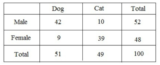
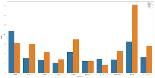
Contingency tables (also called crosstabs or two-way tables) are used in statistics to summarise the relationship between several categorical variables. 

An example of a contingency table:

A great way to visualise categorical data is to use a bar plot/chart, which looks something like this:

There are two main hypothesis tests for categorical data:

Chi-squared test

Fisher exact test

Chi-squared test:

Compares the distribution of two categorical variables in a contingency table to see if they are related e.g. smoking and prevalence of lung cancer. 

Measures difference between what is actually observed in the data and what would be expected if there was truly no relationship between the variables.

Fisher exact test:

Is used instead of Chi-squared when >20% of cells have expected values of <5, or any cell has a count of <1.

If you want to compare several contingency tables for repeated tests of independence i.e. when you have data that you've repeated at different times or locations, you can use the Cochran-Mantel-Haenszel test. 

More detail:

In this situation, there are three nominal categorical variables: the two variables of the contingency test of independence, and the third nominal variable that identifies the repeats (such as different times, different locations, or different studies). For example, you conduct an experiment in winter to see whether legwarmers reduce arthritis. With just one set of people, you'd have two nominal variables (legwarmers vs. control, reduced pain vs. same level of pain), each with two values. If you repeated the same experiment in spring, with a new group, and then again in summer, you would have an added variable: different seasons and groups. You could just add the data together and do a Fisher's exact test, but it would be better to keep each of the three experiments separate. Maybe legwarmers work in the winter but not in the summer, or maybe your first set of volunteers had worse arthritis than your second and third sets etc. In addition, combining different studies together can show a "significant" difference in proportions when there isn't one, or even show the opposite of a true difference. This is known as Simpson's paradox. To avoid this, it's better to use the Cochran-Mantel-Haenszel for this type of data.

Testing for normality in continuous data

The first thing you should do before you do ANYTHING else with your continuous data, is determine whether it is or isn’t normally distributed, this will in turn help you choose the correct significance test to analyse your data. 

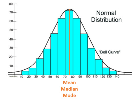
A normal (also known as parametric) distribution is a symmetric distribution where most of the observations cluster around the central peak and the probabilities for values further away from the mean taper off equally in both directions. If plotted, this will look like a symmetrical bell-shaped graph:

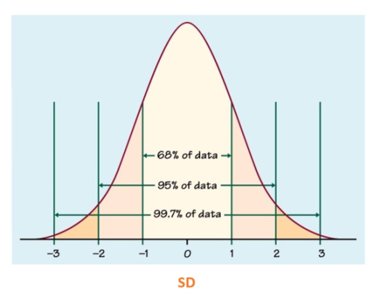
A standard deviation (SD) can be calculated to measure the amount of variation or dispersion of a set of values from the mean. The main and most important purpose of this is to understand how spread out a data set is; a high SD implies that, on average, data points are all pretty far from the average. The opposite is true for a low SD means most points are very close to the average. Generally, smaller variability is better because it represents more precise measurements and yields more accurate analyses.. 

In a normal distribution, SD will look something like this:

In a normal distribution, skewness (measure of assymetry) and kurtosis (the sharpness of the peak) should be equal to or close to 0, otherwise it becomes a variable distribution.

Testing for normality

Various graphical methods are available to assess the normality of a distribution. The main ones are:

A histogram, which will look something like this:

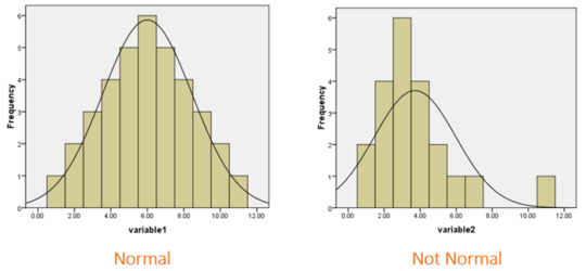
Histograms help visually identify whether the data is normally distributed based on the aforementioned skewness and kurtosis. 

A Q-Q plot:

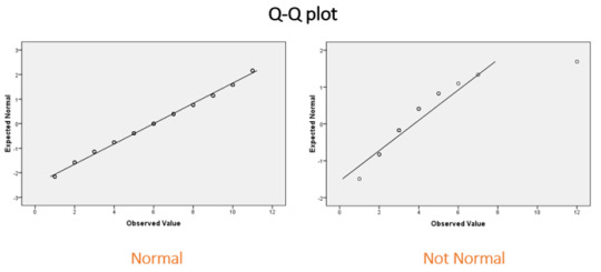
Q-Q plots allow to compare the quantiles of a data set against a theoretical normal distribution. If the majority of points lie on the diagonal line then the data are approximately normal.

and...

A box plot:

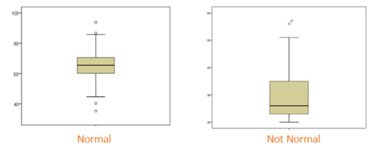
A box plot is an excellent way of displaying continuous data when you are interested in the spread of your data. The thick horizontal bar indicates the median, the top and bottom of the box indicate the interquartile range, and the whiskers represent the spread of data outside of this interquartile range. The dots beyond the whiskers represent outliers, which represent observations that are distant from other observations.

A disadvantage of the box plot is that you don’t see the exact data points. However, box plots are very useful in large datasets where plotting all of the data may give an unclear picture of the shape of your data.

A violin plot is sometimes used in conjunction with the box plot to show density information.

Keep in mind that for real-life data, the results are unlikely to give a perfect plot, so some degree of judgement and prior experience with the data type are required. 

Significance tests

Aside from graphical methods, there are also significance tests, which are used to test for normality. These tests compare data to a normal distribution, whereby if the result is significant the distribution is NOT normal. 

The three most common tests are:

Shapiro-Wilk Test (sample size <5000)

Anderson-Darling Test (sample size > or = 20)

Kolmogorov-Smirnov Test (sample size > or = 1000)

Significance tests for continuous variables

A quick guide for choosing the appropriate test for your data set:

t-test - normally distributed (parametric) data

There are three types of t-test

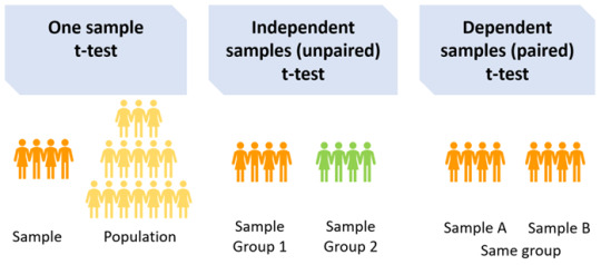
One sample t-test: Compares the mean of the sample with a pre-specified value (population mean) e.g. if the average score of medical students in UK universities is 72 and you want to test whether the average score of medical students in your university is higher/lower, you would need to specify the population mean, in this case 72, when running your t-test.   

A two-sample t-test: Should be used if you want to compare the measurements of two populations. There are two types of the two-sample t-test: paired (dependent) and independent (unpaired). To make the correct choice, you need to understand your underlying data.

Dependent samples t-test (paired): Compares the mean between two dependent groups e.g. comparing the average score of medical students at the University of Sheffield before and after attending a revision course, or comparing the mean blood pressure of patients before and after treatment. Independent samples t-test (unpaired): Compares the mean between two independent groups e.g. average score of medical students between University of Sheffield and the University of Leeds, or comparing the mean response of two groups of patients to treatment vs. control in a clinical trial.

There are several assumptions for the independent (unpaired) t-test:

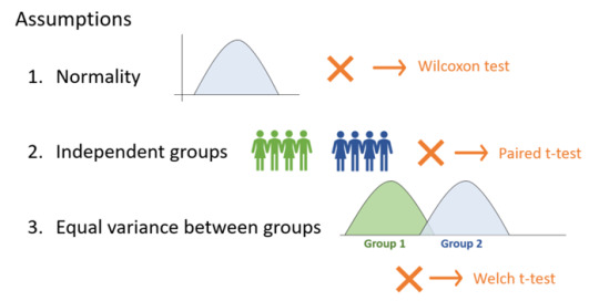
The t-test assumes that the data has equal variance and relies on the data to be normally-distributed. If there isn’t sufficient confidence in this assumption, there are different statistical tests that can be applied. Rather than calculating and comparing the means and variances of different groups they are rank-based methods. However, they still come with a set of assumptions and involve the generation of test statistics and p-values.

Welch t-test, for instance, assumes differences in variance. 

Wilcoxon test (also commonly known as the Mann-Whitney U test) can be used when the data is not normally distributed. This test should not be confused with the Wilcoxon signed rank test (which is used for paired tests). 

The assumptions of the Wilcoxon/Mann-Whitney U test are as follows:

The dependent variable is ordinal or continuous.

The data consist of a randomly selected sample of independent observations from two independent groups.

The dependent variables for the two independent groups share a similar shape.

Summary of the above:

ANOVA - normally distributed (parametric) data

Like the t-test, there are several types of ANOVA tests:

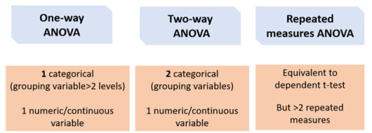
One-way ANOVA:

Equivalent to the independent t-test but for > 2 groups. If you want to compare more than two groups, a one-way ANOVA can be used to simultaneously compare all groups, rather than carrying out several individual two-sample t-tests e.g. to compare the mean of average scores of medical students between the University of Sheffield, the University of Leeds, and the University of Manchester.

The main advantage of doing this is that it reduces the number of tests being carried out, meaning that the type I error rate is also reduced.

Two-way ANOVA:  2 categorical (grouping variables) e.g. comparing the average score of medical students between the University of Sheffield, the University of Leeds, and the University of Manchester AND between males and females.

Repeated measures ANOVA

Equivalent to a paired t-test but for >2 repeated measures e.g. comparing the average score of medical students at University of Sheffield for mid-terms, terms, and finals.

If any of the above ANOVA tests produce a significant result, you also need to carry out a Post-Hoc test.

Post-Hoc test e.g. Tukey HSD

A significant ANOVA result it tells us that there is at least on difference in the groups. However, it does not tell us which group is different. For this, we can apply a post-hoc test such as the Tukey HSD (honest significant difference) test, which is a statistical tool used to determine which sets of data produced a statistically significant result...

For example, for the average scores of medical students between the University of Sheffield, the University of Leeds, and the University of Manchester, the Tukey HSD output may look something like this:

This shows a significant difference between medical students in Manchester and Sheffield and between Leeds and Manchester but not Leeds and Sheffield.

Kruskal Wallis and Friedman tests 

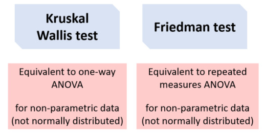
Data that does not meet the assumptions of ANOVA (e.g. normality) can be tested using a non-parametric alternative. The Kruskal-Wallis test is derived from the one-way ANOVA, but uses ranks rather than actual observations. It is also the extension of the Mann-Whitney U test to greater than two groups. Like the one-way ANOVA, this will only tell us that at least one group is different and not specifically which group(s). The Post-Hoc Dunn test is recommended, which also performs a multiple testing correction. For the Friedman test, you can use the Wilcoxon signed-ranks Post-Hoc test. And that is your go-to guide to on how to approach your data! I really hope you find it useful; it definitely helps clarify things for me. ✨

GOOD LUCK!

[gisciencestudent]

Annotated Bibliography of Relevant Sources

Burgan, R, van Wagtendonk, J, Keane, Robert E, Burgan, Robert, & van Wagtendonk, Jan. (2001). Mapping wildland fuels for fire management across multiple scales: Integrating remote sensing, GIS, and biophysical modeling. International Journal of Wildland Fire, 10(3-4), 301–319. https://doi.org/10.1071/WF01028

This study compares the advantages and disadvantages of four different methods of fuel mapping: field reconnaissance, direct remote sensing, indirect remote sensing and biophysical modeling. None of these methods appear to be highly accurate or consistent in and of themselves. Yet, all of these methods represent a means of collecting data for synthesis within a geographic information system for the purpose of creating a map that is useful to land management. The authors propose a strategy which involves classifying biophysical setting, species composition and stand structure to assign fuel models, but acknowledge the enduring need for sensor technology that can penetrate a forest canopy to effectively analyze complex surface fuels.

Church, Richard, Adams, Benjamin, Bassett, Danielle, & Brachman, Micah L. (2019). Wayfinding during a wildfire evacuation. Disaster Prevention and Management., ahead-of-print(ahead-of-print). https://doi.org/10.1108/DPM-07-2019-0216

This will be an interesting article to read when it is published, because it is an example of using GIS to synthesize and analyze empirical data from a wildfire evacuation for the purpose of helping emergency managers to develop more effective wildfire evacuation plans. The authors used network analysis to compare volunteers’ selected routes with the shortest distance routes available, and found that only 31 percent of evacuees took a shortest distance route, and that factors such as the elevation of exits and downhill slope could have impacted wayfinding processes. Although this study is more of a spatiotemporal snapshot, more generalizable results could be produced with additional research.

Coops, Nicholas C., Ferster, Colin J, & Coops, Nicholas C. (2014). Assessing the quality of forest fuel loading data collected using public participation methods and smartphones. International Journal of Wildland Fire, 23(4), 585–590. https://doi.org/10.1071/WF13173

This study looks at the potential for citizens to contribute forest structure and fuels input data for use in the applied geographic information systems used by land managers. Citizen contributions could be especially helpful in data collection over broad areas because accurate characterization of forest fuels is dependent on frequent field measurements, as fuels are spatially variable, can change rapidly due to changing conditions, and are difficult to sense remotely under dense canopy. Eighteen volunteers were recruited at the University of British Colombia, and nine of those had extensive working experience in either wildfire suppression or fuels management. The volunteers used an app on their smartphones to collect and report data. For most components, professional measurements were only slightly closer to reference measurements than volunteered measurements, however, non-professional participants notably overestimated aspect and slope. Overall, when appropriate training is provided and adequate controls for accuracy are incorporated, this study found volunteer data collection to be suitable to help inform forest management decisions.

Danzer, SR, Watts, JM, Stone, S, Yool, SR, Miller, Jay D, Danzer, Shelley R, … Yool, Stephen R. (2003). Cluster analysis of structural stage classes to map wildland fuels in a Madrean ecosystem. Journal of Environmental Management., 68(3), 239–252. https://doi.org/10.1016/S0301-4797(03)00062-8

The authors of this study highlight the importance of quality baseline fuels data since we are not yet capable of assessing understory fuels with remotely sensed data. This assessment therefore combines field data collections with GIS, remote sensing, and hierarchical clustering to map the variability of fuels within and across vegetation types of 156 plots from a mountain range in the southwestern U.S. Vegetation classification was validated using an independent sample of 479 randomly located points and demonstrated substantial accuracy with a Kappa value of .80. However, the overall map, created by combining the land cover/vegetation type classification and fuel classes within vegetation type classifications received a relatively low Kappa of .50. This reduction in accuracy could be attributed to GPS errors, ecological overlap between adjacent vegetation types, and/or confusion of fuel classes in areas where overstory canopies obscured the understory.

Dean, DJ, Blackard, Jock A, & Dean, Denis J. (1999). Comparative accuracies of artificial neural networks and discriminant analysis in predicting forest cover types from cartographic variables. Computers and Electronics in Agriculture., 24(3), 131–151. https://doi.org/10.1016/S0168-1699(99)00046-0

The authors compare an artificial neural networks (ANNs) approach to GIS with a conventional model based on discriminant analysis (DA) with regards to effectiveness at predicting forest cover types. In this study, elevation of each 30x30-m raster cell was obtained directly from USGS digital elevation model (DEM) data. Results demonstrated that both ANN and DA models tended to confuse ponderosa pine, Douglas-fir, and cottonwood/willow cover types with each other, potentially due to geographic proximity. However, overall, the ANN model, with a predictive accuracy of 71.1 percent, was shown to be superior to the DA model, with a predictive accuracy of 58.4 percent.

Eva, E. K. (2010). A method for mapping fire hazard and risk across multiple scales and its application in fire management. Ecological Modelling., 221(1), 2–18. https://doi.org/info:doi/

This study presents an effective approach for mapping fire risk across large, complex geographies containing diverse ecosystems on multiple scales. The author uses FIREHARM, which is a C++ program capable of computing changes in fire characteristics over time using climate data, to predict fuel moisture and corresponding fire behavior, danger, and effects. This model does not provide spatially explicit information concerning fire spread. Instead, it assumes that every pixel or polygon experiences a head fire and simulates the resulting fire characteristics based on ensuing weather factors. A landscape is represented by series of polygons. Each polygon defines an area of similar characteristics (vegetation, fuel, site conditions), is assigned attributes related to fire behavior, and is also assigned a tree list (with attributes of species, diameter, height) which combine to estimate tree mortality for a region. In 2004, FIREHARM was validated by the results of a comparison with 54 sample plots from the Cooney Ridge and Mineral Primm wildfires, producing adequate predictions of fuel consumption within approximately 14 days. The model also had a 60 percent chance of accuracy in predicting canopy vs. non-canopy fire and scorch height and fire severity predictions compared well with observed conditions.

Gatzojannis, S, Galatsidas, S, Kalabokidis, Kostas D, Gatzojannis, Stylianos, & Galatsidas, Spyros. (2002). Introducing wildfire into forest management planning: towards a conceptual approach. Forest Ecology and Management, 158(1-3), 41–50. https://doi.org/10.1016/S0378-1127(00)00715-5

This study explains the process of using a geographic information system to synthesis existing information for the purpose of calculating fire danger and fire resistance per unit area (1 km2) and to map distribution within a forest. First, data is collected, next data is grouped into thematic layers, and finally the layers are synthesized for evaluation. The input data required to produce such a map involves taking an inventory of factors with both horizontal and vertical spatial distribution. Homogeneous information layers, such as landscape, are broken down into a series of variables (vegetation zones, land cover structure, aspect, slope, altitude). External factors include climate, landscape, human impact, and other special factors. Internal factor information layers relate to forest stand structure and describe fire resistance at the forest floor, understory, low crown, middle crown, and high crown levels. The mapping of these factors allows for spatial delineation of fire danger zones which decision makers in determining operational objectives and priorities for large geographical areas.

Ilavajhala, Shriram, Wong, Min Minnie, Justice, Christopher O., Davies, DK, Ilavajhala, S, Min Minnie Wong, & Justice, CO. (2009). Fire Information for Resource Management System: Archiving and Distributing MODIS Active Fire Data. IEEE Transactions on Geoscience and Remote Sensing a Publication of the IEEE Geoscience and Remote Sensing Society., 47(1), 72–79. https://doi.org/10.1109/TGRS.2008.2002076

This paper describes the ways in which the combined technologies of remote sensing and GIS are able to deliver Moderate-resolution Imaging Spectroradiometer (MODIS) active fire data to resource managers and even e-mail customized alerts to users. When used as a mobile service, Fire Information for Resource Management System (FIRMS) is an application that can deliver fire information to field staff regarding potential danger. For example, in South Africa, when a fire is detected either using data from MODIS or from a weather satellite, a text message is sent to relevant personnel who can decide if/what action may be required. This strategy makes satellite-derived FIRMS data more accessible to natural resource managers, scientists, and policy makers who use the data for monitoring purposes and for strategic planning.

Kalabokidis, K. (2013). Virtual Fire: A web-based GIS platform for forest fire control. Ecological Informatics., 16, 62–69. https://doi.org/info:doi/

This research project, supported by the University of Athens in Greece and funded by Microsoft Research, describes the high-tech but user-friendly Virtual Fire system, a web-based GIS platform, which allows firefighting forces to share and utilize real-time data (provided by GPS, satellite, camera) for the purpose of locating resources (vehicles, aircrafts, water tanks) and associated shortest routes, monitoring fire ignition probability, and identifying high risk areas. Data from automatic weather stations also aids in fire prevention and early warning. With the ability to conveniently access this information in synthesized form, managers can design more effective and efficient operational plans. Future considerations involve moving to a cloud-based platform, which would allow for expansion to a broader area and the increased incorporation of mobile devices.

Karlsson Martin, Oskar, Galiana Martin, Luis, Montiel Molina, Cristina, Karlsson Martín, Oskar, & Galiana Martín, Luis. (2019). Regional fire scenarios in Spain: Linking landscape dynamics and fire regime for wildfire risk management. Journal of Environmental Management., 233, 427–439. https://doi.org/10.1016/j.jenvman.2018.12.066

The authors of this study apply socioecological systems theory to the wildfire generations model, which describes and explains the appearance and transformation of large wildfires in relation to landscape dynamics within Mediterranean climatic regions. There is a focus on acknowledging the ways in which humans directly and indirectly affect fire regimes. National forest inventory data and existing maps are the data used to create fire scenarios for the Central Mountain Range in Spain via ArcGIS and SPSS23. Land use and land cover features, which relate certain fuel structures to certain fire behaviors, are assigned to 91 discrete geographical units. The resulting visual comparisons can be used to help managers optimize prevention and suppression strategies.

Koukoulas, Sotirios, Kazanis, Dimitrios, & Arianoutsou, Margarita. (2011). Evaluating Post-Fire Forest Resilience Using GIS and Multi-Criteria Analysis: An Example from Cape Sounion National Park, Greece. Environmental Management., 47(3), 384–397. https://doi.org/10.1007/s00267-011-9614-7

The ability to assess an ecosystem’s resilience, or its capacity to endure disturbances without a state change, is becoming more important in the face of an accelerated decrease in biodiversity and with the projected effects of climate change. This study uses geographic information systems (GIS) to assess post-fire resilience by synthesizing bioindicators, such as forest cover, density, and species richness with geo-indicators, such as fire history, slope, and parent material. The significance of each factor was assessed using sensitivity analysis in order to produce a map of areas at risk- “risk hotspots” – of losing resilience, allowing managers to prioritize resources in restoration efforts.

Kulakowski, D, Veblen, TT, Bigler, Christof, Kulakowski, Dominik, & Veblen, Thomas T. (2005). MULTIPLE DISTURBANCE INTERACTIONS AND DROUGHT INFLUENCE FIRE SEVERITY IN ROCKY MOUNTAIN SUBALPINE FORESTS. Ecology., 86(11), 3018–3029. https://doi.org/10.1890/05-0011

GIS technologies are especially helpful for spatially predicting indicators such as fire severity, which can be the result of complex interactions. This study examines the possible combined effects of interactions between the disturbances of fire, insect outbreaks, and storm blowdown upon fire severity. Pairwise overlay analyses were performed in order to assess these associations. The regression models created, unlike bivariate overlay analysis, allowed for the simultaneous predictions, hypothesis tests and assessment of effects. Results showed that local forest cover type was a significant factor affecting fire spread and severity in the Rocky Mountains, with Spruce-fir stands having the highest probability of burning at high severity. Maps created in GIS show weather variability only significantly affecting fire when fuel build up is sufficient. Pre-fire disturbance and topography were also found to influence burn severity and explain variability.

Michener, W. K. (1997). Quantitatively Evaluating Restoration Experiments: Research Design, Statistical Analysis, and Data Management Considerations. Restoration Ecology : the Journal of the Society for Ecological Restoration., 5(4), 324–337. https://doi.org/10.1046/j.1526-100X.1997.00546.x

Ecological restoration projects (i.e. post-wildfire disturbance) can be very difficult to design and analyze quantitatively due to several factors: experimental units are often heterogeneous, multiple non-uniform treatments may be applied iteratively, replication is difficult or impossible, the effects of extrinsic and intrinsic disturbances may be poorly understood, and the goal of focus is typically the variability in system responses rather than mean responses. This author provides thorough explanations of each of these challenges, along with a variety of ways in which they might be addressed, including via the application of GIS technologies. GIS is described as a powerful tool in relation to this discipline because of its ability to quickly synthesis data using multiple layers, rename and reclassify attributes, analyze spatial coincidence and proximity, and provide quantitative and statistical measurements which can be used to identify potential restoration sites and to visualize and interpret results.

Schroeder, P, Kern, JS, Brown, Sandra L, Schroeder, Paul, & Kern, Jeffrey S. (1999). Spatial distribution of biomass in forests of the eastern USA. Forest Ecology and Management, 123(1), 81–90. https://doi.org/10.1016/S0378-1127(99)00017-1

Biomass is defined by the net difference between photosynthetic production and consumption (respiration, mortality, harvest, herbivory). This measurement is an important indicator of the carbon stored in forests, which can be released as atmospheric carbon into the air during a disturbance (i.e. wildfire) or function as atmospheric carbon sinks during periods of regeneration post-disturbance. While accurate measurements of biomass provide valuable information for decision makers and land managers, large scale estimations can be challenging (remote sensing techniques have met with little success). The authors of this widely-cited study decided to use preciously established methods to convert US forest inventory volume data into above and belowground biomass, downloaded from the USFS Forest Inventory and Analysis (FIA) database, which they then mapped in a geographic information system (GIS) by county. These maps provide a vivid visual representation of forest biomass density patterns over space which can be useful in predicting changes to the global carbon cycle and evaluating potential for increased biomass-carbon storage.

Smith, JE, Weinstein, DA, Laurence, JA, Woodbury, Peter B, Smith, James E, Weinstein, David A, & Laurence, John A. (1998). Assessing potential climate change effects on loblolly pine growth: A probabilistic regional modeling approach. Forest Ecology and Management, 107(1-3), 99–116. https://doi.org/10.1016/S0378-1127(97)00323-X

In this study, a geographic information system was used to integrate regional data including forest distribution, growth rate, and stand characteristics, provided by the USDA Forest Service, with current and predicted climate data in order to produce four different models predicting the potential effects of climate change upon the loblolly pine across the southern U.S. Results indicated a high likelihood of a 19 to 95 percent decrease in growth rates, varying substantially per region and primarily influenced by a relative change in carbon assimilation and CO2 concentrations. In this case, GIS seems particularly useful for synthesizing existing information from regional surveys and account for uncertainties to produce ecological risk assessments at large scales in a way that is useful to policy and decision makers (vs. lengthy reports that are difficult to parse through).

Williams, D, Barry, D, Kasischke, Eric S, Williams, David, & Barry, Donald. (2002). Analysis of the patterns of large fires in the boreal forest region of Alaska. International Journal of Wildland Fire, 11(2), 131–144. https://doi.org/10.1071/WF02023

This study represents the first attempt to spatially correlate the distribution of fire activity in Alaska with climate, topographic, and vegetation cover features using GIS to provide a realistic assignment of fire cycle (frequency) for 11 distinct Alaskan ecoregions (where 96% of all fire activity occurs). GIS technologies can make use of Alaska’s state-wide initiative to digitize maps of fire perimeters from fire events from 1950 to 1999. Perimeter maps are created using a combination of ground and aerial surveys, and aerial photography or satellite imagery. Geospatial analysis showed fire frequency to be influenced by the complex interaction of elevation, aspect, lightening strike frequency, precipitation, forest cover, and growing season temperature.

Please send comments and questions to Melissa Hannah at hannahm@oregonstate.edu or click "Comments Are Welcome" at the top of the page.

[ayearinlanguage]

A Year in Language, Day 220: Lojban Lojban is a constructed language also know as "the logical language". It has possibly the most developed grammar of any conlang. Its grammar is based on predicate logic and can actually be parsed by systems designed for programming languages. The core vocabulary was created algorithmically, by comparing weighted samples of the 6 most populous world languages (at the time); Arabic, English, Hindi, Russian, Chinese (Mandarin), and Spanish. Lojban was originally devised as a theoretical method to test the hypothesis of language relativity, sometimes also knows as the Sapir-Whorf hypothesis i.e. does the language we speak effect the way we think? Lojban would do this by being the "neutral" language; its grammar is just universal logic and it is capable of expressing every kind of specificity or vagueness found in real world languages. For example: some languages, like most Polynesian languages, distinguish alienable and inalienable possession, the difference in having a car or house vs having a mother or arm. Other languages, like English, don't make this distinction. Thus Lojban can show possession that is explicitly alienable, explicitly inalienable, or unspecified either way. There is a well known (in relevant circles) joke about Lojbanists: How man Lojbanists does it take to change a lightbulb? Two: one to figure out what to change it into and another to figure out what kind of bulb emits broken light. The joke plays on the comprehensiveness and rigid exactness of Lojban grammar. The duplicity of meanings and fuzzy bordered definitions common to natural languages are not tolerated in the almost computer language. Many Lojbanists consider this to be a beutiful aspect of the language, helping people expand their way of thinking. Lojban grammar is complex and often compared to coding, and indeed it has many words that are direct verbal transcriptions of logic and math functions. The core is built of "gismu" the, for lack of better word, verb roots that were derived by algorithm from the six languages above. Gismu can be immediatly recognized by their word structure i.e. number of syllables, presence of consonant clusters, and stress location. A fascinating class of words are the "attitudinals" which belong to the class of Lojban grammatical particles called "cmavo". Attitudinals are words that express direct emotion. English equivalents would be words like "aww" in "aww, that's so sweet" or "Oy" as in "oy, I can't take much more of this". Of course, unlike in English, Lajban attitudinals are numerous, exacting, and can take affixes to derive additional meaning. The inclusion of these phrases into the grammar shows insight into the kind of people who create Lojban: The appropriate use of attitudinals in any language is very hard to teach to foreign speakers, and often something that is acquired through social instincts. The only possible truly fluent users of Lojban attitudinals would be theoretical native speakers growing up in a culturally diverse environment. Such a situation is likely to never exist, and yet these words were added with rigor. The origin of Lojban is a dramatic story. It was originally Loglan (logical language) which started development by one Dr James Cooke Brown in 1955. However upon amassing a following who wished to take the language in places he did not agree with there was a schism which came to legal action when Brown attempted to trademark the language. Though this would end up not standing in court the new sect would rebrand as Lojban. For a more in depth look at both Lojban and the story behind it I highly recommend reading "In the Land of Constructed Language" by Akira Okrent.

[perfectlytinyworkspace]

Metagenomics

purpose: sequence genomes of an entire community when...

...we can't culture the organisms in-vitro to get enough DNA for sequencing, i.e., symbiotic organism conditions require interaction w/ host

...we need to answer questions about the effects of microorganisms on the environment

...we need to look at biological characteristics of symbiotic & competitive relationships

...we need to investigate the effects of the microbiome on human health [i.e., relation between disease and gut microbiome/other 'worlds']

difficulties in sequencing a whole community:

bias for easier-to-sequence individuals

need to correct for genome length

community boundaries & variability

absence of reference genomes & markers

horizontal gene transfer [these should be dropped from meta-data]

avoid some of these issues via targeted approach instead of WGS

metagenomics mechanism: sample collection » data processing

1. collect sample – soil/water, skin swab, stool sample, surgical biopsy, etc.

» more biomass = more DNA = easier to sequence

» consider host:microbe biomass ratio when collecting | mucosal membrane communities present ratio challenge

2. extract DNA via chemical/physical lysis » differing levels of lysis ease can introduce early bias in community's measured genomic ratios

3. sequence DNA via 2nd [multiple samples simultaneously! so add indexing labels lol] or 3rd gen sequencing

4. assembly

5. analysis via several different processes

» binning contigs by taxonomy:

for species with available reference genes & sequences, align contigs to known genomic sequences/markers

machine learning/clustering to bring unsequenced species w/ no known references together

generally conducted using analysis of k-mer frequencies and characteristics

» sequenced species: species w/ known genomes can be identified w/o genome assembly simply through matching seq to ref genome

» classify genes by function to gather practical information about community

6. quantify species & functional genes from analysis | relative quantification only because absolute quantities cannot be determined :(

7. Statistic relation [multivariant statistics & machine learning techniques] to previously collected sample metadata to validate background & respond to hypothesis

principle component analysis (PCA) – clustering samples by species/gene composition ratios/frequencies to determine broad changes in species compositions within community as related to differing host environments

correlation studies between different species/genes using gathered metadata

challenges of linking metadata w/ metagenomics + potential solutions:

species bias in the community || soln: different analyses & seq methods

variability & noise [age, sex, diet, phenotype, enviro, medication, etc]/ distinguishing false positives || soln: standardize health records & metadata, conduct longitudinal & controlled animal studies

causality vs correlation: disease causes community? community causes disease? one occurs in tandem with the other but not because of it?

practical metagenomics applications:

environmental science: carbon/nitrogen cycling & global warming role

basic biology: species competition & symbiosis

health science: antibiotic discovery, impacts on human disease

inflammatory & autoimmune diseases [crohn's disease, ulcerative colitis, colon cancer]

autism spectrum disorder, mental health conditions

[sciforce]

Reinforcement Learning and Asynchronous Actor-Critic Agent (A3C) Algorithm, Explained

While supervised and unsupervised machine learning is a much more widespread practice among enterprises today, reinforcement learning (RL), as a goal-oriented ML technique, finds its application in mundane real-world activities. Gameplay, robotics, dialogue systems, autonomous vehicles, personalization, industrial automation, predictive maintenance, and medicine are among RL's target areas. In this blog post, we provide a concrete explanation of RL, its applications, and Asynchronous Actor-Critic Agent (A3C), one of the state-of-the art algorithms developed by Google's DeepMind.

Key Terms and Concepts

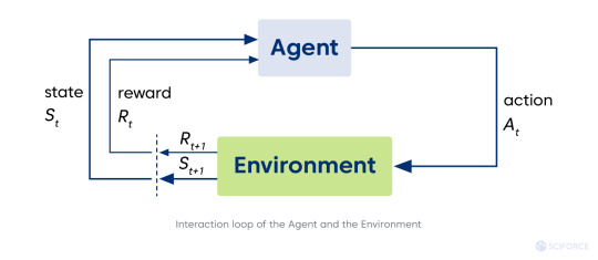
Reinforcement learning refers to the type of machine learning technique enabling an agent to learn to interact with an environment (area outside the agent's borders) by trial and error using reward (feedback from its actions and experiences). The agent seeks ways to maximize the reward via interacting with the environment instead of analyzing the data provided. The agent is a learning controller taking actions in the environment and receives feedback in the form of reward.

The environment, space where the agent gets everything needed from a given state. The environment can be static or dynamic, and its changes can be stochastic and deterministic correspondingly. It is usually formulated as Markov decision process (MDP), a mathematical framework for decision-making development.

However, real-world situations often do not convey information to commit a decision (some context is left behind the currently observed scene). Hence, the Partially Observable Markov Decision Processes (POMDPs) framework comes on the scene. In POMDP the agent needs to take into account probability distribution over states. In cases where it’s impossible to know that distribution, RL researchers use a sequence of multiple observations and actions to represent a current state (i.e., stack of image frames from a game) to better understand a situation. It makes possible to use RL methods as if we are dealing with MDP.

The reward is a scalar value that agents receive from the environment, and it depends on the environment’s current state (St ), the action the agent has performed grounding on the current state (At ), and the following state of the environment (St+1):

Policy (π) stands for an agent’s strategy of behavior at a given time. It is a mapping from the state to the actions to be taken to reach the next state. Speaking formally, it is a probability distribution over actions in a given state, meaning the likelihood of every action in a particular state. In short, policy holds an answer to the “How to act?” question for an agent.

State-value function and action-value function are the ways to assess the policy, as RL aims to learn the best policy. Value function V holds an answer to the question “How good current state is?”, namely an expected return starting from the state (S) and following policy (π).

Sebastian Dittert defines the action-value of a state as “the expected return if the agent chooses action A according to a policy π.” Correspondingly, it is the answer to “How good current action is?”

Thus, the goal of an agent is to find the policy () maximizing the expected return (E[R]). Through the multiple iterations, the agent’s strategy becomes more successful.

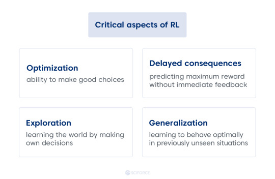
One of the most crucial trade-offs for RL is balancing between exploration and exploitation. In short, exploration in RL aims at collecting experience from new, previously unseen regions. It potentially holds cons like a risk, nothing new to learn, and no guarantee to get any useful further information. On the contrary, exploitation updates model parameters according to gathered experience. In its turn, it does not provide any new data and could not be efficient in case of scarce rewards. An ideal approach is making an agent explore the environment until being able to commit an optimal decision.

Reinforcement Learning vs. Supervised and Unsupervised Learning

Comparing RL with AI planning, the latter does cover all aspects, but not the exploration. It leads to computing the right sequence of decisions based on the model indicating the impact on the environment.

Supervised machine learning involves only optimization and generalization via learning from the previous experience, guided with the correct labels. The agent is learning from its experience based on the given dataset. This ML technique is more task-oriented and applicable for recognition, predictive analytics, and dialogue systems. It is an excellent option to solve the problems having the reference points or ground truth.

Similarly, unsupervised machine learning also involves only optimization and generalization but having no labels referring to the environment. It is data-oriented and applicable for anomaly and pattern discovery, clustering, autoencoders, association, and hyper-personalization pattern of AI.

Asynchronous Advantage Actor-Critic (A3C) Algorithm

The A3C algorithm is one of RL's state-of-the-art algorithms, which beats DQN in few domains (for example, Atari domain, look at the fifth page of a classic paper by Google Deep Mind). Also, A3C can be beneficial in experiments that involve some global network optimization with different environments in parallel for generalization purposes. Here is the magic behind it:

Asynchronous stands for the principal difference of this algorithm from DQN, where a single neural network interacts with a single environment. On the contrary, in this case, we've got a global network with multiple agents having their own set of parameters. It creates every agent's situation interacting with its environment and harvesting the different and unique learning experience for overall training. That also deals partially with RL sample correlation, a big problem for neural networks, which are optimized under the assumption that input samples are independent of each other (not possible in games).

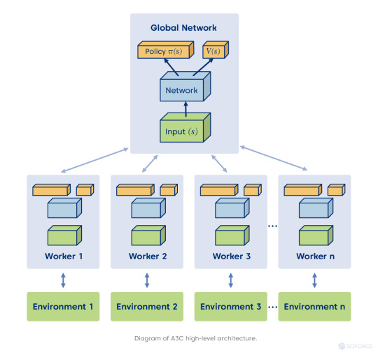
Actor-Critic stands for two neural networks — Actor and Critic. The goal of the first one is in optimizing the policy (“How to act?”), and the latter aims at optimizing the value (“How good action is?”). Thus, it creates a complementary situation for an agent to gain the best experience of fast learning.

Advantage: imagine that advantage is the value that brings us an answer to the question: “How much better the reward for an agent is than it could be expected?” It is the other factor of making the overall situation better for an agent. In this way, the agent learns which actions were rewarding or penalizing for it. Formally it looks like this:

Q(s, a) stands for the expected future reward of taking action at a particular state

V(s) stands for the value of being in a specific state

Challenges and Opportunities

Reinforcement learning’s first application areas are gameplay and robotics, which is not surprising as it needs a lot of simulated data. Meanwhile, today RL applies for mundane tasks like planning, navigation, optimization, and scenario simulation in various verticals chains. For instance, Amazon used it for their logistics and warehouse operations’ optimization and for developing autonomous drone delivery.

Simultaneously, RL still poses challenging questions for industries to answer later. Given its exploratory nature, it is not applicable in some areas yet. Here are some reasons:

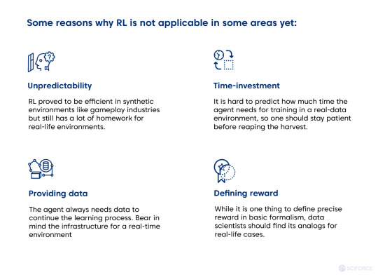
Meanwhile, RL seems to be worth time and resources investment as industry players like Amazon show. Just give it some time, since investment in knowledge always requires it.

[annieboltonworld]

Juniper Publishers- Open Access Journal of Environmental Sciences & Natural Resources

Hydrogeochemical Processes of Evolution Of Ground Water In A Small Tropical Coral Island Of Amini, Union Territory Of Lakshadweep, India

Authored by Joji VS

Abstract

In the small tropical island of Amini ground water occurs under phreatic condition and is seen as a thin lens floating over the saline water. The coral sands and coral limestone act as principal aquifers. The depth of the wells varies from 1.6 to 5.5 mbgl and depth to the water table 1.20 to 4.80 mbgl. The ground water is generally alkaline and EC varies from 465 to 999 micromhos /cm at 25o C. The ground water is under Na+- SO42- type and shallow to deep meteoric percolation types and generally alkaline in nature. The factors affecting the quality of ground water are rainfall, tides, ground water recharge and draft, human and animal wastes, oil spills and fertilizers. Water samples collected from different parts of the island during pre-monsoon and post monsoon seasons. The water sample results of chemical analysis indicate that water type ranges from Ca-HCO3 (recharge type) to Ca-Mg-Cl type (reverse ion exchange water type). The hydrochemistry is mainly controlled by evaporation, partly influenced by water-rock interaction and aquifer materials. The evaporation process played major role in the evolution of water chemistry. The ground water in the study area is generally suitable irrigation for all types of soil.

Keywords: Atoll; Fresh water lens; Chloro alkali indices; Base exchange indices and Irrigation

Introduction

The Lakshadweep islands (LD islands) are a group of tiny coral islands, located in the Arabian Sea, about 400 km from the main land (southern tip of the Indian peninsula). They spread over a distance of 300 km, consists of 36 coral islands and a number of sunken banks, open coral reef and sand banks. These islands are typically a chain of low islands surrounding a shallow lagoon, consisting of large recent sediments on top of older coral limestone. Amini Island has a delicate ecosystem with very limited fresh water resources. Though the island receives high rainfall, lack of surface storage and the limited ground water storage capacity, where fresh water is occurring as a small lens floating over saline water, makes fresh water a precious commodity. High porosity of the aquifers allow mixing of freshwater with sea water and due to high population density, waste water gets mixed with the fresh water in the aquifer, make the management of the limited fresh water resources multifaceted.

The purpose of the study is to assess the evolution of ground water resources of the island and to know the hydro geological characteristics. The Small Island hydro geological and hydro chemical studies were carried out by many authors at international and regional levels. These include Nura Umar Kura et al. 2013 on Evaluation of Factors Influencing the Groundwater Chemistry in a Small Tropical Island of Malaysia [1], applied factor analysis tool to the hydro chemical data set of Manukan Island in order to extract the principal factors corresponding to the different sources of variation in the hydrochemistry, Belkhiria et al. 2012 studied geochemical evolution of groundwater in an alluvial aquifer in the case of El Eulma aquifer, East Algeria, [2] used application of multivariate statistical techniques in the assessment of groundwater quality in seawater intrusion area in Bafra Plain, Turkey [3] carried out assessment of groundwater quality for Veppanthattai taluk, Perambalur district, Tamil Nadu using Remote Sensing and GIS, [4] on fresh water - salt water relation, [5] Appraisal of groundwater resources in an island condition and many others. The present study is an attempt to highlight hydro geochemical processes of evolution groundwater in a small tropical coral island of Amini, Union Territory of Lakshadweep, India.

Study area

Amini Island is the sixth largest of the inhabited islands of the UT of Lakshadweep, with an area of 2.50 Km2 and is elliptical in shape. Amini island is located between Kadmath and Kavarati (in the N-S direction) and between Agathi and Androth (in the E-W direction) in a NE-SW alignment, about 11 km south of Kadmath island. It is about 58 km SW of Kiltan Island. It is 294 km from Mangalore, 324 km from Kozhikode and 407 km from Kochi. It is located between north latitudes 110 07' 00" and 11008'00" and east longitude 720 44' 00" and 720 45' 00". The climate of Amini is similar to the climatic conditions of Kerala. March to May is the hottest period of the year. The temperature ranges from 25oC to 35oC and humidity ranging from 70 -76 per cent for most of the year. The average rainfall received is 1600 mm a year. Monsoon prevails here from 15th May to 15th September. During the monsoon time, boats are not allowed outside the lagoon because of the violent sea. The presence of the reef maintains calm at the lagoon.

The location map of LD islands including Amini Island is compiled (Figure 1) and various salient features of Amini are compiled (Table 1). The coral island is the work of minute sea organisms called coral polyps and they congregate in large colonies. When the organisms die, their skeletons, which are made of limestone, form big clusters, some of which rise above the water. Charles Darwin first described the different types of coral reef after his voyage by HMS Beagle among the Galapagos Isles in Pacific Ocean (Subsidence theory for the origin of coral In oceanic island fresh ground water occurs as a lens floating over saline water. The hydro dynamic balance of fresh and saline water determines the shape and movement of interface and may be controlled by some of the following factors viz. water table fluctuation due to diurnal tides, seasonal fluctuation of water table due to recharge or draft, dispersion and molecular diffusion. Due to these factors there is an alternate up and down movement of the interface.

Materials and Methods

The base map of Amini and various layers were prepared by using Map Info 6.5 techniques and in the ground water resource of Amini has been computed based on the methodology recommended by the GEC 1997. The recharge to ground water lens = rain fall - interception - evapotranspiration and Ground water utilisation = Evapotranspiration + mixing + pumping + outflow, for water balance study monthly water budgeting or weekly water budgeting gives appropriate value of recharge. The main consumer of ground water is coconut palms because one coconut tree consumes 40 lpd and density of coconut trees is 25 000 - 35000 sq. km but draft through plant is slow, steady and spread uniformly.

The various hydro geological parameters collected during the field study and water level data observed during low and high tide. The pre-monsoon groundwater samples collected from shallow aquifers (dug wells) in polyethylene bottles and analysed for pH, EC, F-, Cl-, NO3-, HCO3-, SO42-, Ca2+, Mg2+, Na+, and K+ as per standard procedures (APHA, 1995) and the in-situ measurements of EC and pH were carried out by using EC and pH meters. The total dissolved solids were estimated by ionic calculation methods. The F-, Cl- and NO3- ions were determined by ion selective electrode; HCO3- by potentiometric titration; SO42- by modified titration method after [6,7]; Ca2+ and Mg2+ in absorption mode while Na+ and K+ in emission mode of the atomic absorption spectrophotometer. The analytical results were tested for accuracy by calculating the Normalized Inorganic Charge Balance [8]. The analytical precision was such that the ion charge balance was little above ±5% for the samples. The quality of the analysis was ensured by standardization using blank, spike, and duplicate samples.

Results and Discussion

The major factors influence the hydrological characteristics of the island are climate, humidity, temperature, evapotranspiration, physiography, hydro geological aspects, soil, vegetation, population geomorphology, aquifer nature and human interference. The major hydrochemistry is discussed below.

Climate, humidity, temperature, evapotranspiration, physiography, hydro geological aspects, soil, vegetation, population, geomorphology, aquifer nature and human interference

The climate of a small island is one of the major influences on the availability of naturally occurring freshwater resources [9]. The rainfall distribution, quantity and its spatial and temporal variations and the evapotranspiration play an important role on the availability of the freshwater resources. The climate of Amini is similar to the climatic conditions of Kerala. March to May is the hottest period of the year. The temperature ranges from 25oC to 35oC and humidity ranging from 70 -76 per cent for most of the year. The average rainfall received is 1600 mm a year. Monsoon prevails here from 15th May to 15th September. The monsoon period raises temperature to the mercury level between 2730 degrees. During the monsoon time, boats are not allowed outside the lagoon because of the violent sea. The presence of the reef maintains calm at the lagoon. The evapotranspiration is very high and most of the months except in high rainfall season it exceeds the rainfall making the water surplus on the negative side.

The entire LD islands lay on the northern edge of the 2500 km long North-South aligned submarine Lakshadweep- Chagos ridge. The island has coarse sandy soil of high porosity and permeability resulting in little or no surface runoff. The vegetation of LD islands consists of coconut trees, bushes and grasses. The Amini Island is a typical atoll and height of the land above msl is about 1-2 m and the coral sands and the coral limestone act as principal aquifers. The Ghyben-Herzberg relation determines the depth of the interface between fresh water and sea water. The water level data of monitoring wells in Amini Island reveals that depth of the wells ranges from 1.6 to 5.5 mbgl and the DTW ranges between 1.2 to 4.8 mbgl whereas diurnal fluctuation in water level due to tides is in the range of 0 to 80 cms. The climate water balance method of recharge estimation widely used for estimating the recharge on small islands Falkland 1992. Human activities influence both the availability of freshwater and water quality.

Hydro geochemical processes

The hydro geochemical processes of ground water and its evolution have been examined. The groundwater of different geological horizons can be classified depending upon their ionic strength of select anions and [10] categorized groundwater based on the meq/l content of Cl- , SO42- , and HCO3- . The water is Normal chloride type if Cl- is <15 meq/l, Normal sulphate type if SO42- is <6 meq/l and Normal bicarbonate type if HCO3- varies between 2 and 7 meq/l. Distribution of groundwater samples based on the Soltan's classification has indicated that majority of the samples are of Normal chloride type, followed by Normal bicarbonate type (values rounded off) and concentration of salts in natural waters depend on the geology, environment, and movement of water [11,12].

The base exchange indices, r1(r1 = Na+ - Cl-/ SO42- meq/ l) and r2 (r2 = K+ + Na+ - Cl- SO42- meq/l) after [13] could be applied for the further classification of groundwater. The groundwater can be grouped as Na+ - HCO3- type if r1 > 1 and Na+- SO4- type with r1 < 1; r2 < 1- groundwater is of deep meteoric percolation type and >1, shallow meteoric percolation type. The groundwater of the area comes Na+- SO4 - type type and deep meteoric percolation type except a few one which is deep meteoric percolation type, chemical analysis data of ground water and other details are compiled (Tables 2 & 3). Hydro chemical evolution study based on Na+ / Cl- molar ratio Na+ / Cl- molar ratio will be 1 if halite dissolution is responsible for sodium dominance in groundwater and >1 if Na+ is released from silicate weathering process [14]. The Na+ / Cl- molar ratio is <1 in many samples of the season, indicating that halite dissolution was the primary process responsible for the release of Na+ into the groundwater.

Hydro chemical facies

The groundwater is further evaluated to determine its facies by plotting the percentages of select chemical constituents in Modified Piper diagram [15]. The plots for the PRS season indicated distribution within the fields 5 and 6 of the Chadha's diagram (Figures 2a & 2b) and are characterized by alkaline earths and weak acidic anions exceed both alkali metals and strong acidic anions, respectively i.e (Ca+Mg)+ (CO3+HCO3)> (Na +K) +( Cl+SO4) and the sample at Ammini - Sidiqui Palli with alkaline earths exceed alkali metals and strong acidic anions exceed weak acidic anions ie (Ca+Mg)>(Na+K)>(Cl+SO4)>(CO3+HCO3). All the water samples of PSM are falling under field 5. All the samples except Ammini - Sidiqui Palli falling under Sub-field I and are Ca-HCO3 Type / recharge type water but that of Ammini - Sidiqui Palli falling under sub-field II Sub-field II and is Ca-Mg-Cl type, reverse ion exchange type. The plots also suggest that among cations Ca+ and Na+ and anions HCO3- and Cl - dominate the ionic concentration in groundwater.

Hydro geochemical evaluation

The high sodium content among cations in the groundwater for the period could be due to halite dissolution which was further enhanced by evaporation and/or evapotranspiration processes. The Na+ /Cl- molar ratio will be 1 if halite dissolution is responsible for sodium dominance in groundwater and >1 if Na+ is released from silicate weathering process Meybeck 1987. The Na+ / Cl- molar ratio is >1 in the samples of water can only evolve to brine rich in NaCl if it encounters highly soluble chloride minerals, typically associated with evaporative deposits / evaporates [16]. As all the groundwater samples of the season with Na+ /Cl- molar ratio less than one or nearer to one, halite dissolution is responsible for sodium dominance in groundwater of the small coral island of Amini, Union Territory of Lakshadweep.

Evolution of groundwater

[17] plots, in which TDS vs Na+ /(Na+ +Ca2+ ) for cations and TDS vs Cl- /(Cl- + HCO3 - ) for anion were plotted to know evolution process of the groundwater and the influence of host rock on ground water chemistry. It is revealed that the samples, occupied the evaporation dominance field. The rock water interaction played minimum role in the evolution of water chemistry, which was dominated by evaporation process during PRM and PSM. The geological location is one of the most important factors affecting the groundwater quality [18].

Chloro alkali indices

The role of aquifer material in the evolution of groundwater chemical composition has been examined by determining the chloro alkali indices for cations (CAI-1) and anions (CAI-2). The CAI-1 [Cl- - (Na+ + K+ )]Cl- and CAI-2 [Cl- - (Na+ + K+ )/(SO42- + HCO3- + CO3 - + NO- )], developed by [19], relate the ion exchange process between ground water and aquifer material. The CAI-1 and CAI-2 are negative in the samples indicating the ion exchange between Na+ -K+ in water and Ca2+ -Mg2+ in rocks [20]. It is imperative to understand the modifications in water chemistry during its movement and residency time for better evaluation of the hydrochemistry of any area more so when different geological formations are involved in a watershed or river basin [21]. As CAI-1 and CAI-2 are negative in the samples of PSM indicating the ion exchange predominance in the study area during post-monsoon and positive values during PRM shown lesser role of ion exchange during pre-monsoon.

Irrigation Suitability: The irrigation suitability of ground water has been attempted based on the study of electrical conductivity (EC), Sodium Adsorption Ratio (SAR), Percent Sodium (% Na), Permeability index (PI), Kelley's Index (KI), Soluble Sodium Percentage (SSP) and Magnesium Ratio (MR) methodologies (Table 4) and Wilcox classification of irrigation water and U S Salinity diagram for irrigation Water, methodology and analytical results are compiled (Table 5).

Electrical conductivity: The EC is a measure of salinity hazard to crops and classified into five major types, as per Raghunath 1987 and that the samples in the study area are under excellent, good, permissible and doubtful categories.

Sodium Absorption Ratio, SAR: The sodium alkali hazard or Sodium Absorption Ratio (SAR) of water is an indicator of sodium hazard in irrigation water Gholami and Srikantaswamy 2009. As per Richard 1954, the computed SAR values show that all the samples are excellent.

Percent Sodium (% Na): The % Na is used to assess the ground water quality, because a higher level of sodium in irrigation water may increase the exchange of sodium content of irrigated soil and affect soil permeability, structure and create toxic condition for plants [22,23] and Todd 1980. Based on the relative proportions of cation concentration, samples come under excellent to good categories and can be used for irrigation on almost all types of soil.

Permeability index, PI: Doneen 1964 has classified the irrigation water quality into three classes based on permeability- class I, II and III and all the samples come under Class II and suitable for irrigation in all types of soil.

Kelley's Index, KI: Kelley 1940 and Paliwal 1967 proposed the suitability of irrigation water quality based on the sodium concentration against calcium and magnesium. The water is suitable for irrigation if KI value is <1; water with KI value of >1 is considered as of poor quality for irrigation and >2 KI makes the water unsuitable for irrigation. Both cation exchange and reverse ion exchange are encouraged by aquifer materials and land use practices, in waterlogged area, marshy/swampy land, creek, mud/tidal flat represented by Montmorillonite clays, which lead to the release of Na or Ca into groundwater and adsorption of Ca or Na, respectively Alison et al. 1992. In all samples KI values are below 1 indicating the water in the study area is suitable for irrigation.

Soluble Sodium Percentage, SSP: Water with less than or equal to 50 SSP value is of good quality and more than 50 is not suitable for irrigation as permeability will be very low [24-26]. In the study area all the water samples with SSP values less than 50.

Magnesium Ratio MR: Water with less than or equal to 50 MR value is of good quality and >50 is considered unsuitable for irrigation Lloyd and Heathcote et al. 1985. In the study area majority of the water samples except one water sample with MR values less than 50.

Conclusion

Hydrogeochemical processes of evolution of groundwater in in the small coral island ofAmini, Union Territory ofLakshadweep, India has been examined. The Amini island is of coral origin (a typical atoll) and ground water occurs under phreatic condition floats as thin lens over saline water and is abstracted mainly by open dug wells. The DWT in the island varies from 1.20 to 4.80 mbgl and depth of the wells varies from less than two meters to about 5.5 mbgl and is controlled by tides. The ground water in the island is generally alkaline ranges from 465 to 999 micromhos / cm at 25 o C. The factors affecting the quality are rainfall, tides, ground water recharge and draft, human and animal wastes, oil spills and fertilizers. The groundwater samples of different areas are of Na- SO4 Type and deep meteoric percolation type. The ground water in the area is mainly Ca-HCO3 type / recharge type water and Ca-Mg-Cl type (reverse ion exchange water type. The hydrochemistry is mainly controlled by evaporation, followed by water-rock interaction and aquifer material.

For more articles in Open Access Journal of Environmental Sciences & Natural Resources please click on: https://juniperpublishers.com/ijesnr/index.php

[iampaulbrown]

Supervised vs unsupervised machine learning

Supervised and unsupervised learning are the two different types of tasks in machine learning. In short supervised learning is done when we have prior knowledge of what the output values for our samples should be, and therefore, the goal of supervised learning is to learn a function that best approximates the relationship between input and output observable in the data. Unsupervised learning, on the other hand, does not have labeled outputs, so its goal is to infer the natural structure present within a set of data points.

Supervised Learning

Supervised learning is typically done in the context of classification, when we want to map input to output labels, or regression, when we want to map input to a continuous output. Common algorithms in supervised learning include logistic regression, naive bayes, support vector machines, artificial neural networks, and random forests. In both regression and classification, the goal is to find specific relationships or structure in the input data that allow us to effectively produce correct output data. 

When conducting supervised learning, the main considerations are model complexity, and the bias-variance tradeoff. Note that both of these are interrelated.

Model complexity refers to the complexity of the function you are attempting to learn - similar to the degree of a polynomial. The proper level of model complexity is generally determined by the nature of your training data. If you have a small amount of data, or if your data is not uniformly spread throughout different possible scenarios, you should opt for a low-complexity model. This is because a high-complexity model will overfit if used on a small number of data points. 

The bias-variance tradeoff also relates to model generalisation. In any model, there is a balance between bias, which is the constant error term, and variance, which is the amount by which the error may vary between different training sets. So, high bias and low variance would be a model that is consistently wrong 20% of the time, whereas a low bias and high variance model would be a model that can be wrong anywhere from 5%-50% of the time, depending on the data used to train it.

Unsupervised Learning

The most common tasks within unsupervised learning are clustering, representation learning, and density estimation. In all of these cases, we wish to learn the inherent structure of our data without using explicitly-provided labels. Some common algorithms include k-means clustering, principal component analysis, and auto-encoders. Since no labels are provided, there is no specific way to compare model performance in most unsupervised learning methods.

Two common use-cases for unsupervised learning are exploratory analysis and dimensionality reduction.

Unsupervised learning is very useful in exploratory analysis because it can automatically identify structure in data. For example, if an analyst were trying to segment consumers, unsupervised clustering methods would be a great starting point for their analysis. In situations where it is either impossible or impractical for a human to propose trends in the data, unsupervised learning can provide initial insights that can then be used to test individual hypotheses.

Dimensionality reduction, which refers to the methods used to represent data using less columns or features, can be accomplished through unsupervised methods. In representation learning, we wish to learn relationships between individual features, allowing us to represent our data using the latent features that interrelate our initial features. This sparse latent structure is often represented using far fewer features than we started with, so it can make further data processing much less intensive, and can eliminate redundant features.

So in summary:

Supervised: All data is labeled and the algorithms learn to predict the output from the input data.

Unsupervised: All data is unlabelled and the algorithms learn to inherent structure from the input data.

[newscheckz]

What is semi-supervised machine learning?

New Post has been published on https://newscheckz.com/what-is-semi-supervised-machine-learning/

What is semi-supervised machine learning?

Machine learning has proven to be very efficient at classifying images and other unstructured data, a task that is very difficult to handle with classic rule-based software.

But before machine learning models can perform classification tasks, they need to be trained on a lot of annotated examples.

Data annotation is a slow and manual process that requires humans to review training examples one by one and giving them their right labels.

In fact, data annotation is such a vital part of machine learning that the growing popularity of the technology has given rise to a huge market for labeled data.

From Amazon’s Mechanical Turk to startups such as LabelBox, ScaleAI, and Samasource, there are dozens of platforms and companies whose job is to annotate data to train machine learning systems.

Fortunately, for some classification tasks, you don’t need to label all your training examples.

Instead, you can use semi-supervised learning, a machine learning technique that can automate the data-labeling process with a bit of help.

Supervised vs unsupervised vs semi-supervised machine learning

You only need labeled examples for supervised machine learning tasks, where you must specify the ground truth for your AI model during training. Examples of supervised learning tasks include image classification, facial recognition, sales forecasting, customer churn prediction, and spam detection.

Unsupervised learning, on the other hand, deals with situations where you don’t know the ground truth and want to use machine learning models to find relevant patterns. Examples of unsupervised learning include customer segmentation, anomaly detection in network traffic, and content recommendation.

Semi-supervised learning stands somewhere between the two. It solves classification problems, which means you’ll ultimately need a supervised learning algorithm for the task.

But at the same time, you want to train your model without labeling every single training example, for which you’ll get help from unsupervised machine learning techniques.

Semi-supervised learning with clustering and classification algorithms

One way to do semi-supervised learning is to combine clustering and classification algorithms.

Clustering algorithms are unsupervised machine learning techniques that group data together based on their similarities.

The clustering model will help us find the most relevant samples in our data set. We can then label those and use them to train our supervised machine learning model for the classification task.

Say we want to train a machine learning model to classify handwritten digits, but all we have is a large data set of unlabeled images of digits.

Annotating every example is out of the question and we want to use semi-supervised learning to create your AI model.

First, we use k-means clustering to group our samples. K-means is a fast and efficient unsupervised learning algorithm, which means it doesn’t require any labels.

K-means calculates the similarity between our samples by measuring the distance between their features.

In the case of our handwritten digits, every pixel will be considered a feature, so a 20×20-pixel image will be composed of 400 features.

  K-means clustering is a machine learning algorithm that arranges unlabeled data points around a specific number of clusters.

  When training the k-means model, you must specify how many clusters you want to divide your data into. Naturally, since we’re dealing with digits, our first impulse might be to choose ten clusters for our model.

But bear in mind that some digits can be drawn in different ways. For instance, here are different ways you can draw the digits 4, 7, and 2.

You can also think of various ways to draw 1, 3, and 9.

Therefore, in general, the number of clusters you choose for the k-means machine learning model should be greater than the number of classes.

In our case, we’ll choose 50 clusters, which should be enough to cover different ways digits are drawn.

After training the k-means model, our data will be divided into 50 clusters. Each cluster in a k-means model has a centroid, a set of values that represent the average of all features in that cluster.

We choose the most representative image in each cluster, which happens to be the one closest to the centroid. This leaves us with 50 images of handwritten digits.

Now, we can label these 50 images and use them to train our second machine learning model, the classifier, which can be a logistic regression model, an artificial neural network, a support vector machine, a decision tree, or any other kind of supervised learning engine.

Training a machine learning model on 50 examples instead of thousands of images might sound like a terrible idea.

But since the k-means model chose the 50 images that were most representative of the distributions of our training data set, the result of the machine learning model will be remarkable.

In fact, the above example, which was adapted from the excellent book Hands-on Machine Learning with Scikit-Learn, Keras, and Tensorflow, shows that training a regression model on only 50 samples selected by the clustering algorithm results in a 92-percent accuracy (you can find the implementation in Python in this Jupyter Notebook).

In contrast, training the model on 50 randomly selected samples results in 80-85-percent accuracy.

But we can still get more out of our semi-supervised learning system. After we label the representative samples of each cluster, we can propagate the same label to other samples in the same cluster.

Using this method, we can annotate thousands of training examples with a few lines of code. This will further improve the performance of our machine learning model.

Other semi-supervised machine learning techniques

There are other ways to do semi-supervised learning, including semi-supervised support vector machines (S3VM), a technique introduced at the 1998 NIPS conference.

S3VM is a complicated technique and beyond the scope of this article. But the general idea is simple and not very different from what we just saw: You have a training data set composed of labeled and unlabeled samples.

S3VM uses the information from the labeled data set to calculate the class of the unlabeled data, and then uses this new information to further refine the training data set.

  The semi-supervised support vector machine (S3VM) uses labeled data to approximate and adjust the classes of unlabeled data.

  If you’re are interested in semi-supervised support vector machines, see the original paper and read Chapter 7 of Machine Learning Algorithms, which explores different variations of support vector machines (an implementation of S3VM in Python can be found here).

An alternative approach is to train a machine learning model on the labeled portion of your data set, then using the same model to generate labels for the unlabeled portion of your data set. You can then use the complete data set to train an new model.

The limits of semi-supervised machine learning

Semi-supervised learning is not applicable to all supervised learning tasks. As in the case of the handwritten digits, your classes should be able to be separated through clustering techniques.

Alternatively, as in S3VM, you must have enough labeled examples, and those examples must cover a fair represent the data generation process of the problem space.

But when the problem is complicated and your labeled data are not representative of the entire distribution, semi-supervised learning will not help.

For instance, if you want to classify color images of objects that look different from various angles, then semi-supervised learning might help much unless you have a good deal of labeled data (but if you already have a large volume of labeled data, then why use semi-supervised learning?).

Unfortunately, many real-world applications fall in the latter category, which is why data labeling jobs won’t go away any time soon.

But semi-supervised learning still has plenty of uses in areas such as simple image classification and document classification tasks where automating the data-labeling process is possible.

Semi-supervised learning is a brilliant technique that can come handy if you know when to use it.

This article was originally published by Ben Dickson on TechTalks, a publication that examines trends in technology, how they affect the way we live and do business, and the problems they solve. But we also discuss the evil side of technology, the darker implications of new tech and what we need to look out for. You can read the original article here. 

[globalmediacampaign]

Enabling low code graph data apps with Amazon Neptune and Graphistry

One of the common challenges to unlocking the value of graph databases is building easy-to-use, customer-facing data tools that expose graph-powered insights in impactful and visual ways. Data engineers need to inspect data quality, data scientists need to perform discovery and inspect models, analysts need to investigate connections, and managers need insight into what’s going on. The ability for a project to make data easily accessible is often the difference between reaching many users in your organization vs. having little return on your project. However, all too often, creating these data applications isn’t easy, as trying to combine the required components together quickly turns into a slog. Recently, Graphistry released a new open-source tool, graph-app-kit, which aims to solve this problem by providing a low code way to create powerful data applications for your Amazon Neptune managed graph database. graph-app-kit pairs the simplicity of a Streamlit data app, with point-and-click visual analytics tools of the GPU-accelerated Graphistry platform, all backed by a robust and scalable graph database in Neptune. The combination enables you to investigate your graph while performing analytical operations, such as viewing key clusters, as shown in the following animation. The GPU acceleration provided by Graphistry means even large Neptune results can be visually analyzed in a web browser. In this post, we demonstrate how to use graph-app-kit to generate a full-stack dashboard, complete with GPU-backed graph analytics on top of Neptune. We cover the process of launching Neptune, configuring and launching graph-app-kit, and building your first dashboard, by only modifying a few lines of code. For our data, we build upon the identity graph used in the post Building a customer identity graph with Amazon Neptune to construct an interactive enterprise-ready data dashboard that can be made available to business users like security and fraud, sales and marketing, and supply chain and logistics. Overview of solution Before we dive into the details, let’s first take a moment to answer the question: What is graph-app-kit? graph-app-kit is an open-source software project that integrates best-of-breed tools in the Python data science ecosystem: Streamlit dashboarding with Jupyter notebook authoring Tabular and graph analytics packages, including the RAPIDS GPU ecosystem with cuDF, cuGraph, and Graphistry for GPU visual graph analytics Database adapters, such as for Neptune, for a robust and scalable graph database optimized for storing billions or relationships and querying them with millisecond latency The core of graph-app-kit is a Docker host used to run all these technologies. Docker provides standardized configuration, launching, and operation, resulting in a quick-to-deploy system. The architecture of a deployed graph-app-kit instance consists of five containers: The first of these containers is a reverse proxy server, using Caddy, which directs incoming requests to one of four backend containers. Two of these containers run Streamlit dashboards, one configured to serve public-facing dashboards and the other configured to serve private password-protected dashboards. The remaining two containers are part of the Graphistry platform. One of these containers runs the Graphistry platform, while the other runs a Jupyter server that is used to interact with both Graphistry. The following diagram shows the architecture of the launched graph-app-kit stack for Neptune. This post covers the latest version of graph-app-kit, but for any future changes and potential customizations, we suggest you refer to the graph-app-kit tutorials in the GitHub repo. To get started deploying this stack, we have provided AWS CloudFormation templates for both Neptune and graph-app-kit, which make it easy to launch and manage your stacks. When you create this stack, you will be responsible for AWS charges incurred. Launching Neptune (optional if using an existing cluster) The first step in our deployment is to create our Neptune cluster and load the identity dataset. This data, such as the device identifiers, browsers, cookies, and history of sites visited or mobile apps used, represents a unique identity for a collection of users. This data also contains known demographics about the user based on information provided through various account profiles. This data is highly connected and is similar to what you might find via web server logs or clickstream data, as shown below. To use a GPU, you must selection an AWS region with a GPU quota. If you already have a Neptune instance with identity data, you can skip ahead to the next step. Launch Neptune with the preloaded identity data from the identity graph tutorial. Choose the stack for your preferred Region: Region View Launch US East (Ohio) View US East (N. Virginia) View US West (Oregon) View EU (Ireland) View In the Capabilities section, select the two check-boxes that grant the stack permissions to create the AWS Identity and Access Management (IAM) roles. Choose Create stack. The process of creating your stack may take up to 20 minutes to complete. When the process is complete, open the generated Identity-Graph-Sample stack’s Outputs It displays the values you need to configure graph-app-kit: VPC – ID vpc-abc PublicSubnet1 – ID subnet-abc DBClusterReadEndpoint – URL abc.cluster-ro-xyz.zzz.neptune.amazonaws.com To facilitate a fast bulk load of the sizable identity dataset, this CloudFormation script uses a Neptune cluster with an r5.12xlarge instance. After you complete this step, we recommend resizing the Neptune instance size to an r5.2xlarge to reduce the overall cost. You can view the Amazon Neptune costs on the pricing page. Launching graph-app-kit The CloudFormation template uses the Graphistry Core offering in the AWS Marketplace, which requires you accept its terms and conditions. After we launch Neptune, we’re ready to configure and launch graph-app-kit. Launch graph-app-kit for the Region where your Neptune cluster resides and you have GPU EC2 instances enabled: Region View Launch US East (Ohio) View US East (N. Virginia) View US West (Oregon) View EU (Ireland) View Fill in the launch settings using the output values you recorded earlier and select the instance size. Make sure that the VPC and subnet chosen are capable of connecting to the VPC of your Neptune cluster and that the subnet is the public subnet, so that you are able to access graph-app-kit from the internet. The least expensive self-managed GPU and Graphistry configuration for graph-app-kit is g4dn.xlarge (EC2 pricing information). To further lower costs by going CPU-only and with a free Graphistry Hub account, see Configuration 2: Minimal. Choose Create Stack to begin the stack creation. If your account isn’t configured for GPU capacity, you can launch a minimal CPU-only version of graph-app-kit with a subset of the components. Launching graph-app-kit may take up to 10 minutes to complete. To monitor the progress of the installation, SSH into the instance (user ubuntu) and run the following code: tail -f /var/log/cloud-init-output.log -n 1000 When the stack creation is complete, the public IP address is available on the stack’s Outputs tab on the AWS CloudFormation console. With graph-app-kit deployed, the following features are now available: All public dashboards can be viewed at http://[the.public.ip.address]/public/dash Private dashboards are available after logging in at http://[the.public.ip.address]/private/dash You can access notebooks to live-edit dashboards at http://[the.public.ip.address]/notebook Administrator functions are located at http://[the.public.ip.address]/admin The default login credentials for protected pages are admin / i-theInstanceID and should be changed upon first login. Sample Gremlin dashboard graph-app-kit runs Python-based dashboards using Streamlit. Let’s take a look at one of the dashboards that comes out of the box with graph-app-kit. From the drop-down menu, choose Gremlin: Simple Sample. A view is shown with a layout consisting controls on the left that filter the data, in this case a slider for the number of edges to show, and a main content area that shows filtered data, in this case the Graphistry browser. Changing the filtering controls causes the dashboard to populate the Graphistry browser with data from the Neptune database. Creating a new dashboard One of the top use cases for a graph data app is enabling users to filter data by predefined attributes and visually explore the resulting graph. We’ve looked at a very simple dashboard with a single filter, but in many cases, you want to have multiple different criteria to refine your filter. Let’s see how we can extend that view to add additional filters to our dashboard. For this post, we copy and modify the existing view of our sample Gremlin database to add the ability to filter our results by state. The process of creating most new dashboards is easy to accomplish and involves the following steps: Clone the existing view, in this case the Gremlin sample. Register the new view in Streamlit. Add or modify any filtering UI controls. For this post, we add a drop-down menu to filter by state. Update the view’s query to incorporate the filter control values. Cloning the Gremlin sample view using Jupyter’s file browser To create our new view, named Blog Search Demo, we copy an existing Gremlin sample view. You can accomplish this by a variety of methods, but for this post, we use Jupyter, which is included as part of graph-app-kit. Go to http://[the.public.ip.address]/notebook/tree/notebooks/graph-app-kit/public/views/ , and log in. From the New drop-down folder, choose Folder. Choose the generated folder Untitled. Choose Rename. Enter blog_search_demo. Navigate to http://[the.public.ip.address]/notebook/tree/notebooks/graph-app-kit/public/views/demo_neptune_01_minimal_gremlin. Choose Duplicate and Duplicate selected. Select our newly duplicated file and choose Move. Move it to /notebooks/graph-app-kit/public/views/blog_search_demo. Go to your new folder blog_search_demo and select the copied file. Rename it to _init_py. Registering the new view in Streamlit Now that we have created a copy of this view, we need to register this view with Streamlit by giving it a name and unique application ID. The name property is the name of the dashboard in the UI, and app_id is used for the lexicographic sort order of dashboards on the dashboard drop-down menu. To change these properties for our new view, complete the following steps: Using Jupyter’s file browser, choose the file _init_.py to open it for editing. At the top of the file, make the following changes: For app_id, change app_neptune_01 to blog_search. For name, change GREMLIN: Simple Sample to Blog - Faceted search. Save the file. Go to http://[[the.public.ip.address]]/public/dash. From the drop-down menu, choose Blog – Faceted Search to refresh your browser to the new view. Adding the filter control Most graph-app-kit views are variants of the same flow: show filters, pass their settings to a query runner, then pass the query results to a main area results renderer. In our example, we need to add a new filter control to the sidebar_area() method and incorporate the new filter into our query, which we complete in the following sections. Our first step is to add a new filtering control to the sidebar by editing the sidebar_area() method. Out of the box, Streamlit comes with a variety of different filter controls such as sliders, drop-downs, and text boxes, which we can use to add additional filtering criteria to our application. For this post, we add a new drop-down menu containing the states to the UI by adding the st.sidebar.selectbox() call to our method. If we want the filter value to be part of the URL, such as for when sharing links, we can also copy the URL init and set pattern used in the next lines for the num_edges UI control. Finally, we expose the filter controls’ value by returning from sidebar_area() method. See the following code: def sidebar_area(): state = st.sidebar.selectbox( 'Find users from this state?', [ 'All States', 'Alabama', 'Alaska', … Additional States omitted for brevity... 'Wisconsin', 'Wyoming' ]) num_edges_init = urlParams.get_field('num_matches', 10000) … Updating the Gremlin query to incorporate the filter With our new filter UI control in place, we update the query to utilize this new filter. First, we add the new filter setting state into the method signature for run_filters(). Next, we add an additional step to our Gremlin traversal to include the filtering criteria when it is set. The following code shows our updated method: def run_filters(num_edges, state): g, conn = gremlin_helper.connect_to_neptune() logger.info('Querying neptune') t = g.V().inE() if not state == "All States": t = t.has('visited', 'state', state) res = t.limit(num_edges).outV().path().by( __.valueMap().with_(WithOptions.tokens)).toList() nodes_df, edges_df = path_to_df(res) ... When we save the file and reload the browser, our users can now filter data by state and see the results. The following screenshot shows the interactive dashboard with custom state filter. Examining this visualization quickly reveals the top clusters in the filtered identity graph. Although not covered in this post, graph-app-kit also includes examples of how to integrate additional GPU-accelerated analytics projects common in the RAPIDS ecosystem, such as cuGraph and BlazingSQL. The dashboard examples show using GPU acceleration to make analytical and machine learning UIs interactive on larger data. Conclusion When you add up the blue lines of code, this was surprisingly little work. graph-app-kit took care of the plumbing, all the way through deployment, data pipeline, and the UI. Your team can focus on just repeating the short graph-app-kit process for your custom view. Being able to quickly share purpose-built tools means more of your users can finally leverage the power of graph analysis and drive insights from their business data. In this post, we showed you how to do the following: Launch a full graph dashboarding stack in your private cloud Create a new Streamlit view straight from Jupyter Add a new UI filter control Run a custom Gremlin graph query over your Neptune graph database Show the results with GPU-accelerated interactive graph visualization using Graphistry’s Python client As you bring graph data to more of your organization, join us in the Graphistry community chat and feel free to contribute your extensions! If you have any questions, comments, or other feedback, we’re always available through your Amazon account manager or via the Neptune Discussion Forums. About the Authors Leo Meyerovich is the founder and CEO of Graphistry Inc for 100X’ing investigations with GPU-accelerated visual graph analytics and workflow automation. His previous research in high-performance computing, security verification, and programming language design received awards including SIGPLAN 10 Year Test of Time and multiple best-paper awards.     Dave Bechberger is a Sr. Graph Architect with the Amazon Neptune team. He used his years of experience working with customers to build graph database-backed applications as inspiration to co-author “Graph Databases in Action” by Manning.     Taylor Riggan is a Sr. Specialist Solutions Architect focusing on graph databases at AWS. He works with customers of all sizes to help them learn and use purpose-built NoSQL databases via the creation of reference architectures, sample solutions, and delivering hands-on workshops.   https://aws.amazon.com/blogs/database/enabling-low-code-graph-data-apps-with-amazon-neptune-and-graphistry/

[back7up]

Medical Education Curriculum Model Support for Medical Student Retention Capacity

Medicine education is a vast and continuously evolving with appropriate medical curriculum required to support the learning process of medical students. Nowadays, many curriculum models are developed and used in medical education. However, the development of a new curriculum model must be accompanied by an evaluation process to obtain feedback and adjust the curriculum regularly.

This research was conducted at a medical education institution with a bachelor’s degree medical program, which carried out two curriculum models as part of the transition period following the curriculum redesign process. The old curriculum gives material in one full semester with integrated modules and the new curriculum with a cluster system (1-2 basic courses offered in a certain period) and system-organ blocks.

Currently, there are still no studies comparing the old curriculum and new curriculum in terms of retention capacity. So this is our basis to find out which curriculum model supports medical students in terms of retention capacity.

We used two groups of students (2nd year and 3rd year) as a sample in this study. The chosen subject is Clinical Pathology. This topic is one of the necessary medical science materials given at relatively the same time to both groups.

In the first group (3rd-year students), clinical Pathology courses are given for 14 weeks, along with seven other subjects. Whereas in the second group (2nd-year students), Clinical Pathology courses are provided for six weeks along with one other course. The material and method of examination evaluation between the first and second groups are the same.

Retention tests were conducted five months after the two groups had completed the Clinical Pathology course. This test consists of 25 multiple choice questions that cover the entire Clinical Pathology material. Correct answers will be given a value of +1, and there are no penalties for blank or incorrect answers. The fundamental difference between a retention test and a final course exam is a retention test; the questions are aimed at testing students’ understanding of Clinical Pathology material. This test does not assess the ability of students to memorize the topic.

The retention test was attended by 280 students, consisting of 138 3rd year students and 142 2nd year students. From the test results, it was found that the mean retention test scores in the first group were significantly higher than the second group (10.93 ± 3.57 vs. 8.56 ± 3.19, p

Based on the above results, it can be concluded that the ability of the retention of knowledge about the clinical pathology of students in the first group is better than the second group. Some of the things that we suspect cause differences between the first group and the second group are: (1) Load of material and available time, (2) Number of courses carried out simultaneously, and (3) Other factors that affect individual learning experiences.

Regarding the material load and the time needed to process it, there is a cognitive load theory proposed by Merriënboer et al. (2010). It was stated that the human brain only has limited capacity to store information in a moment (working memory) in a certain period. For data to be processed into long-term memory, repetition is needed so that working memory is not ignored or forgotten, but is converted to long-term memory.

The variation in the number of courses given in parallel can also affect student retention abilities. With the increasing number of courses, students are expected to be able to integrate the knowledge gained from one course to another, so they get a general picture of the material they are learning.

Besides, other factors that play a role are individual learning experiences. Such as (1) Individual factors consisting of motivation, learning routines, and habits of repeating material after lecture; (2) teaching factors such as teaching style, guidance given by instructors, and the use of instruments in the teaching process; (3) Learning environment; and (4) Other factors such as family problems or health problems.

The medical curriculum model may have a significant impact on the capacity of medical student retention capacity. To have better retention capabilities, we must consider the material and time to process it. (*)

Authors: Jovian Philip Swatan, Fundhy Sinar Ikrar Prihatanto, Nancy Margarita Rehatta, and Atika

Journal articles can be accessed through the following pages: https://doi.org/10.3946/kjme.2019.145

This article was originally published on http://news.unair.ac.id/en/2020/03/04/medical-education-curriculum-model-support-for-medical-student-retention-capacity/

[mariebenz]

How Best to Measure Patient Persistence with Medications? Self Report or Pharmacy Fill?

MedicalResearch.com Interview with:

Dr. Fanaroll Alexander C. Fanaroff, MD, MHS Assistant Professor of Medicine, Division of Cardiovascular Medicine University of Pennsylvania MedicalResearch.com: What is the background for this study? Response: This is a secondary analysis of the ARTEMIS, a cluster randomized trial of copayment assistance for P2Y12 inhibitors in patients that had myocardial infarction. One of the primary endpoints of ARTEMIS was persistence with P2Y12 inhibitors: Did the patient continue to take a P2Y12 inhibitor over the entire 1 year following MI? In ARTEMIS, we captured persistence data in two ways, patient report and pharmacy fill records. What we did in this study was to look at the agreement between persistence as measured by these two methods. MedicalResearch.com: What are the main findings? Response: Overall, 15% of patients self-reported non-persistence, but 48% of patients were non-persistent by pharmacy fill data. When we looked at agreement between the methods, the two methods quite frequently did not agree:  50% of patients were persistent by both methods, 13.5% were non-persistent by both methods, 34.8% reported that they were persistent but were non-persistent by pharmacy fill, and 1.8% reported that they were non-persistent but were actually persistent by pharmacy fill records. Both methods are subject to bias: Self-report is subject to social desirability bias (where patients misrepresent medication taking behavior to please investigators) and recall bias (where patients don't remember their medications). Pharmacy fill data is subject to missing data if a pharmacy is not included in the database, or other reasons. Because of these biases, we next tried to understand which method of measuring persistence -- pharmacy fill records or self-report -- was "correct."  To do this, we used two other methods of measuring persistence that were captured in ARTEMIS: copayment assistance vouchers and P2Y12 inhibitor serum drug levels. We had serum drug levels for a random sample of patients in ARTEMIS, and we found limited agreement beyond chance between serum drug levels and persistence as measured by pharmacy fill and patient report, which did not help sort out which method was more "correct." In the intervention arm, patients used vouchers to have copayments for P2Y12 inhibitors waived, and we were able to track when vouchers were used. Using the voucher data, 20% of patients that self-reported persistence but were characterized by pharmacy fill data as non-persistent actually were persistent, suggesting that pharmacy fill data underestimates persistence by roughly that amount. Lastly, we looked at clinical outcomes by persistence category, and found that patients persistent by both methods had the best outcomes, patients non-persistent by both methods had the worst outcomes, and patients with discordant persistence had outcomes intermediate between concordantly persistent and non-persistent patients. MedicalResearch.com: What should readers take away from your report? Response: Electronic health records increasingly have a mechanism for enabling physicians to check pharmacy fill records for patients to track persistence with medications. Our results show that this data is important, as it identifies more patients than self-report, but that it needs to be interpreted somewhat cautiously: Many patients non-persistent by pharmacy fill are actually persistent. The best way to understand persistence is to incorporate both patient self-report and pharmacy fill data, recognizing that patients non-persistent by both methods will have the worst outcomes.   MedicalResearch.com: What recommendations do you have for future research as a result of this work? Response: Currently, health systems employ a number of  interventions to increase medication persistence. Future research should look at the best way to target these interventions to patients that are non-persistent with medications, including methods that use both patient report and pharmacy fill data. No disclosures relevant to this research Citation:  Fanaroff AC, Peterson ED, Kaltenbach LA, et al. Agreement and Accuracy of Medication Persistence Identified by Patient Self-report vs Pharmacy Fill: A Secondary Analysis of the Cluster Randomized ARTEMIS Trial. JAMA Cardiol. Published online March 04, 2020. doi:10.1001/jamacardio.2020.0125   Last Modified:       The information on MedicalResearch.com is provided for educational purposes only, and is in no way intended to diagnose, cure, or treat any medical or other condition. Always seek the advice of your physician or other qualified health and ask your doctor any questions you may have regarding a medical condition. In addition to all other limitations and disclaimers in this agreement, service provider and its third party providers disclaim any liability or loss in connection with the content provided on this website.   Read the full article