#DataFrame Column Removal

[codewithnazam]

How to Drop a Column in Python: Simplifying Data Manipulation

Dive into our latest post on 'Drop Column Python' and master the art of efficiently removing DataFrame columns in Python! Perfect for data analysts and Python enthusiasts. #PythonDataFrame #DataCleaning #PandasTutorial 🐍🔍

Hello, Python enthusiasts and data analysts! Today, we’re tackling a vital topic in data manipulation using Python – how to effectively use the Drop Column Python method. Whether you’re a seasoned programmer or just starting out, understanding this technique is crucial in data preprocessing and analysis. In this post, we’ll delve into the practical use of the drop() function, specifically…

[himanitech]

Wielding Big Data Using PySpark

Introduction to PySpark

PySpark is the Python API for Apache Spark, a distributed computing framework designed to process large-scale data efficiently. It enables parallel data processing across multiple nodes, making it a powerful tool for handling massive datasets.

Why Use PySpark for Big Data?

Scalability: Works across clusters to process petabytes of data.

Speed: Uses in-memory computation to enhance performance.

Flexibility: Supports various data formats and integrates with other big data tools.

Ease of Use: Provides SQL-like querying and DataFrame operations for intuitive data handling.

Setting Up PySpark

To use PySpark, you need to install it and set up a Spark session. Once initialized, Spark allows users to read, process, and analyze large datasets.

Processing Data with PySpark

PySpark can handle different types of data sources such as CSV, JSON, Parquet, and databases. Once data is loaded, users can explore it by checking the schema, summary statistics, and unique values.

Common Data Processing Tasks

Viewing and summarizing datasets.

Handling missing values by dropping or replacing them.

Removing duplicate records.

Filtering, grouping, and sorting data for meaningful insights.

Transforming Data with PySpark

Data can be transformed using SQL-like queries or DataFrame operations. Users can:

Select specific columns for analysis.

Apply conditions to filter out unwanted records.

Group data to find patterns and trends.

Add new calculated columns based on existing data.

Optimizing Performance in PySpark

When working with big data, optimizing performance is crucial. Some strategies include:

Partitioning: Distributing data across multiple partitions for parallel processing.

Caching: Storing intermediate results in memory to speed up repeated computations.

Broadcast Joins: Optimizing joins by broadcasting smaller datasets to all nodes.

Machine Learning with PySpark

PySpark includes MLlib, a machine learning library for big data. It allows users to prepare data, apply machine learning models, and generate predictions. This is useful for tasks such as regression, classification, clustering, and recommendation systems.

Running PySpark on a Cluster

PySpark can run on a single machine or be deployed on a cluster using a distributed computing system like Hadoop YARN. This enables large-scale data processing with improved efficiency.

Conclusion

PySpark provides a powerful platform for handling big data efficiently. With its distributed computing capabilities, it allows users to clean, transform, and analyze large datasets while optimizing performance for scalability.

For Free Tutorials for Programming Languages Visit-https://www.tpointtech.com/

[onemanscienceband]

when i'm in the middle of a programming headache i sometimes return to the question of why do libraries like tidyverse or pandas give me so many headaches

and the best I can crystallize it is like this: the more you simplify something, the more restricted you make its use case, which means any time you want to deviate from the expected use case, it's immediately way harder than it seemed at the start.

like. i have a list and I want to turn it into a dataframe. that's easy, as long as each item in the list represents a row for the dataframe*, you're fine. but what if you want to set a data type for each column at creation time? there's an interface for passing a list of strings to be interpreted as column names, but can I pass a list of types as well?

as far as I can tell, no! there might have been one back in the early 2010s, but that was removed a long time ago.

so instead of doing:

newFrame = pd.DataFrame(dataIn,cols=colNames,types=typeNames)

I have to do this:

newFrame = pd.DataFrame(dataIn,cols=colNames) for colName in ["col1","col2","col3"]: newFrame[colName] = newFrame[colName].astype("category")

like, the expected use case is just "pass it the right data from the start", not "customize the data as you construct the frame". it'd be so much cleaner to just pass it the types I want at creation time! but now I have to do this in-place patch after the fact, because I'm trying to do something the designers decided they didn't want to let the user do with the default constructor.

*oh you BET I've had the headache of trying to build a dataframe column-wise this way

[pabloatech]

4th week: plotting variables

I put here as usual the python script, the results and the comments:

Python script:

Created on Tue Jun 3 09:06:33 2025

@author: PabloATech """

libraries/packages

import pandas import numpy import seaborn import matplotlib.pyplot as plt

read the csv table with pandas:

data = pandas.read_csv('C:/Users/zop2si/Documents/Statistic_tests/nesarc_pds.csv', low_memory=False)

show the dimensions of the data frame:

print() print ("length of the dataframe (number of rows): ", len(data)) #number of observations (rows) print ("Number of columns of the dataframe: ", len(data.columns)) # number of variables (columns)

variables:

variable related to the background of the interviewed people (SES: socioeconomic status):

biological/adopted parents got divorced or stop living together before respondant was 18

data['S1Q2D'] = pandas.to_numeric(data['S1Q2D'], errors='coerce')

variable related to alcohol consumption

HOW OFTEN DRANK ENOUGH TO FEEL INTOXICATED IN LAST 12 MONTHS

data['S2AQ10'] = pandas.to_numeric(data['S2AQ10'], errors='coerce')

variable related to the major depression (low mood I)

EVER HAD 2-WEEK PERIOD WHEN FELT SAD, BLUE, DEPRESSED, OR DOWN MOST OF TIME

data['S4AQ1'] = pandas.to_numeric(data['S4AQ1'], errors='coerce')

NUMBER OF EPISODES OF PATHOLOGICAL GAMBLING

data['S12Q3E'] = pandas.to_numeric(data['S12Q3E'], errors='coerce')

HIGHEST GRADE OR YEAR OF SCHOOL COMPLETED

data['S1Q6A'] = pandas.to_numeric(data['S1Q6A'], errors='coerce')

Choice of thee variables to display its frequency tables:

string_01 = """ Biological/adopted parents got divorced or stop living together before respondant was 18: 1: yes 2: no 9: unknown -> deleted from the analysis blank: unknown """

string_02 = """ HOW OFTEN DRANK ENOUGH TO FEEL INTOXICATED IN LAST 12 MONTHS

Every day

Nearly every day

3 to 4 times a week

2 times a week

Once a week

2 to 3 times a month

Once a month

7 to 11 times in the last year

3 to 6 times in the last year

1 or 2 times in the last year

Never in the last year

Unknown -> deleted from the analysis BL. NA, former drinker or lifetime abstainer """

string_02b = """ HOW MANY DAYS DRANK ENOUGH TO FEEL INTOXICATED IN THE LAST 12 MONTHS: """

string_03 = """ EVER HAD 2-WEEK PERIOD WHEN FELT SAD, BLUE, DEPRESSED, OR DOWN MOST OF TIME:

Yes

No

Unknown -> deleted from the analysis """

string_04 = """ NUMBER OF EPISODES OF PATHOLOGICAL GAMBLING """

string_05 = """ HIGHEST GRADE OR YEAR OF SCHOOL COMPLETED

No formal schooling

Completed grade K, 1 or 2

Completed grade 3 or 4

Completed grade 5 or 6

Completed grade 7

Completed grade 8

Some high school (grades 9-11)

Completed high school

Graduate equivalency degree (GED)

Some college (no degree)

Completed associate or other technical 2-year degree

Completed college (bachelor's degree)

Some graduate or professional studies (completed bachelor's degree but not graduate degree)

Completed graduate or professional degree (master's degree or higher) """

replace unknown values for NaN and remove blanks

data['S1Q2D']=data['S1Q2D'].replace(9, numpy.nan) data['S2AQ10']=data['S2AQ10'].replace(99, numpy.nan) data['S4AQ1']=data['S4AQ1'].replace(9, numpy.nan) data['S12Q3E']=data['S12Q3E'].replace(99, numpy.nan) data['S1Q6A']=data['S1Q6A'].replace(99, numpy.nan)

create a recode for number of intoxications in the last 12 months:

recode1 = {1:365, 2:313, 3:208, 4:104, 5:52, 6:36, 7:12, 8:11, 9:6, 10:2, 11:0} data['S2AQ10'] = data['S2AQ10'].map(recode1)

print(" ") print("Statistical values for varible 02 alcohol intoxications of past 12 months") print(" ") print ('mode: ', data['S2AQ10'].mode()) print ('mean', data['S2AQ10'].mean()) print ('std', data['S2AQ10'].std()) print ('min', data['S2AQ10'].min()) print ('max', data['S2AQ10'].max()) print ('median', data['S2AQ10'].median()) print(" ") print("Statistical values for highest grade of school completed") print ('mode', data['S1Q6A'].mode()) print ('mean', data['S1Q6A'].mean()) print ('std', data['S1Q6A'].std()) print ('min', data['S1Q6A'].min()) print ('max', data['S1Q6A'].max()) print ('median', data['S1Q6A'].median()) print(" ")

plot01 = seaborn.countplot(x="S2AQ10", data=data) plt.xlabel('Alcohol intoxications past 12 months') plt.title('Alcohol intoxications in the Past 12 Months in the NESARC Study')

plot02 = seaborn.countplot(x="S1Q6A", data=data) plt.xlabel('Highest grade (1-14)') plt.title('Highest grade or year of school completed')

I create a copy of the data to be manipulated later

sub1 = data[['S2AQ10','S1Q6A']]

create bins for no intoxication, few intoxications, …

data['S2AQ10'] = pandas.cut(data.S2AQ10, [0, 6, 36, 52, 104, 208, 365], labels=["very few","some", "often", "quite often", "very often", "permanent"])

change format from numeric to categorical

data['S2AQ10'] = data['S2AQ10'].astype('category')

print ('intoxication category counts') c1 = data['S2AQ10'].value_counts(sort=False, dropna=True) print(c1)

bivariate bar graph C->Q

plot03 = seaborn.catplot(x="S2AQ10", y="S1Q6A", data=data, kind="bar", ci=None) plt.xlabel('Alcohol intoxications') plt.ylabel('Highest grade')

c4 = data['S1Q6A'].value_counts(sort=False, dropna=False) print("c4: ", c4) print(" ")

I do sth similar but the way around:

creating 3 level education variable

def edu_level_1 (row): if row['S1Q6A'] <9 : return 1 # high school if row['S1Q6A'] >8 and row['S1Q6A'] <13 : return 2 # bachelor if row['S1Q6A'] >12 : return 3 # master or higher

sub1['edu_level_1'] = sub1.apply (lambda row: edu_level_1 (row),axis=1)

change format from numeric to categorical

sub1['edu_level'] = sub1['edu_level'].astype('category')

plot04 = seaborn.catplot(x="edu_level_1", y="S2AQ10", data=sub1, kind="boxen") plt.ylabel('Alcohol intoxications in the past 12 months') plt.xlabel('Highest grade') plt.grid() plt.show()

Results and comments:

length of the dataframe (number of rows): 43093 Number of columns of the dataframe: 3008

Statistical values for variable "alcohol intoxications of past 12 months":

mode: 0 0.0 dtype: float64 mean 9.115493905630748 std 40.54485720135516 min 0.0 max 365.0 median 0.0

Statistical values for variable "highest grade of school completed":

mode 0 8 dtype: int64 mean 9.451024528345672 std 2.521281770664422 min 1 max 14 median 10.0

intoxication category counts very few 6026 some 2042 often 510 quite often 272 very often 184 permanent 276 Name: S2AQ10, dtype: int64

c4: (counts highest grade)

8 10935 6 1210 12 5251 14 3257 10 8891 13 1526 7 4518 11 3772 5 414 4 931 3 421 9 1612 2 137 1 218 Name: S1Q6A, dtype: int64

Plots: Univariate highest grade:

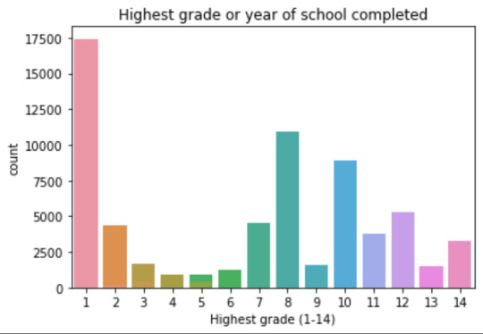
mean 9.45 std 2.5

-> mean and std. dev. are not very useful for this category-distribution. Most interviewed didn´t get any formal schooling, the next larger group completed the high school and the next one was at some college but w/o degree.

Univariate number of alcohol intoxications:

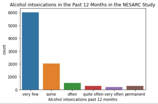
mean 9.12 std 40.54

-> very left skewed, most of the interviewed persons didn´t get intoxicated at all or very few times in the last 12 months (as expected)

Bivariate: the one against the other:

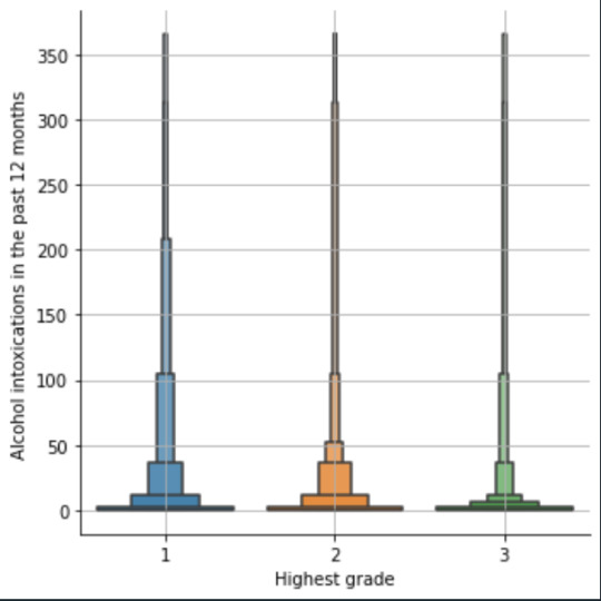
This bivariate plot shows three categories:

1: high school or lower

2: high school to bachelor

3: master or PhD

And the frequency of alcohol intoxications in the past 12 months.

The number of intoxications is higher in the group 1 for all the segments, but from 1 to 3 every group shows occurrences in any number of intoxications. More information and a more detailed analysis would be necessary to make conclusions.

[learning-code-ficusoft]

Data Analysis with Python: A Beginner’s Guide to Pandas

Data Analysis with Python: 

A Beginner’s Guide to Pandas Pandas is a foundational library in Python for data analysis, offering robust tools to work with structured data. 

It simplifies tasks like data cleaning, exploration, and transformation, making it indispensable for beginners and experts alike. 

What is Pandas?

 Pandas is an open-source Python library built for:

 Data Manipulation: Transforming and restructuring datasets. 

Data Analysis: Aggregating, summarizing, and deriving insights from data. Handling Tabular Data: Easily working with structured data, such as tables or CSV files. 

By leveraging Pandas, analysts can focus on solving problems rather than worrying about low-level data-handling complexities. 

Core Concepts in Pandas Data Structures:

 Series: A one-dimensional array with labeled indices. 

Example Use Case: 

Storing a list of items with labels (e.g., prices of products). 

DataFrame: A two-dimensional structure with labeled rows and columns. 

Example Use Case: Representing a table with rows as observations and columns as attributes. 

Data Handling: Loading Data: Pandas supports importing data from various sources like CSV, Excel, SQL databases, and more. 

Data Cleaning: 

Removing duplicates, handling missing values, and correcting data types. 

Data Transformation: 

Filtering, sorting, and applying mathematical or logical operations to reshape datasets. 

Exploratory Data Analysis (EDA): With Pandas, analyzing data trends and patterns becomes simple. 

Examples include: Summarizing data with describe(). Grouping and aggregating data using groupby().

 Why Use Pandas for Data Analysis?

 Ease of Use: 

Pandas provides intuitive, high-level methods for working with data, reducing the need for complex programming. 

Versatility: It supports handling various data formats and seamlessly integrates with other libraries like NumPy, Matplotlib, and Seaborn. Efficiency: Built on top of NumPy, Pandas ensures fast data operations and processing. 

Key Advantages for Beginners Readable Code: 

Pandas uses simple, readable syntax, making it easy for beginners to adopt. Comprehensive 

Documentation: Extensive resources and community support help users quickly learn the library. 

Real-World Applications: Pandas is widely used in industries for financial analysis, machine learning, and business intelligence. 

Theoretical Importance of Pandas Pandas abstracts complex data manipulation into easy-to-use methods, empowering users to: Handle data from raw formats to structured forms. Perform detailed analysis without extensive programming effort. 

Build scalable pipelines for data processing and integration. 

This makes Pandas an essential tool for anyone stepping into the world of data analysis with Python.

WEBSITE: https://www.ficusoft.in/python-training-in-chennai/

[fromdevcom]

Pandas DataFrame Cleanup: Master the Art of Dropping Columns Data cleaning and preprocessing are crucial steps in any data analysis project. When working with pandas DataFrames in Python, you'll often encounter situations where you need to remove unnecessary columns to streamline your dataset. In this comprehensive guide, we'll explore various methods to drop columns in pandas, complete with practical examples and best practices. Understanding the Basics of Column Dropping Before diving into the methods, let's understand why we might need to drop columns: Remove irrelevant features that don't contribute to analysis Eliminate duplicate or redundant information Clean up data before model training Reduce memory usage for large datasets Method 1: Using drop() - The Most Common Approach The drop() method is the most straightforward way to remove columns from a DataFrame. Here's how to use it: pythonCopyimport pandas as pd # Create a sample DataFrame df = pd.DataFrame( 'name': ['John', 'Alice', 'Bob'], 'age': [25, 30, 35], 'city': ['New York', 'London', 'Paris'], 'temp_col': [1, 2, 3] ) # Drop a single column df = df.drop('temp_col', axis=1) # Drop multiple columns df = df.drop(['city', 'age'], axis=1) The axis=1 parameter indicates we're dropping columns (not rows). Remember that drop() returns a new DataFrame by default, so we need to reassign it or use inplace=True. Method 2: Using del Statement - The Quick Solution For quick, permanent column removal, you can use Python's del statement: pythonCopy# Delete a column using del del df['temp_col'] Note that this method modifies the DataFrame directly and cannot be undone. Use it with caution! Method 3: Drop Columns Using pop() - Remove and Return The pop() method removes a column and returns it, which can be useful when you want to store the removed column: pythonCopy# Remove and store a column removed_column = df.pop('temp_col') Advanced Column Dropping Techniques Dropping Multiple Columns with Pattern Matching Sometimes you need to drop columns based on patterns in their names: pythonCopy# Drop columns that start with 'temp_' df = df.drop(columns=df.filter(regex='^temp_').columns) # Drop columns that contain certain text df = df.drop(columns=df.filter(like='unused').columns) Conditional Column Dropping You might want to drop columns based on certain conditions: pythonCopy# Drop columns with more than 50% missing values threshold = len(df) * 0.5 df = df.dropna(axis=1, thresh=threshold) # Drop columns of specific data types df = df.select_dtypes(exclude=['object']) Best Practices for Dropping Columns Make a Copy First pythonCopydf_clean = df.copy() df_clean = df_clean.drop('column_name', axis=1) Use Column Lists for Multiple Drops pythonCopycolumns_to_drop = ['col1', 'col2', 'col3'] df = df.drop(columns=columns_to_drop) Error Handling pythonCopytry: df = df.drop('non_existent_column', axis=1) except KeyError: print("Column not found in DataFrame") Performance Considerations When working with large datasets, consider these performance tips: Use inplace=True to avoid creating copies: pythonCopydf.drop('column_name', axis=1, inplace=True) Drop multiple columns at once rather than one by one: pythonCopy# More efficient df.drop(['col1', 'col2', 'col3'], axis=1, inplace=True) # Less efficient df.drop('col1', axis=1, inplace=True) df.drop('col2', axis=1, inplace=True) df.drop('col3', axis=1, inplace=True) Common Pitfalls and Solutions Dropping Non-existent Columns pythonCopy# Use errors='ignore' to skip non-existent columns df = df.drop('missing_column', axis=1, errors='ignore') Chain Operations Safely pythonCopy# Use method chaining carefully df = (df.drop('col1', axis=1) .drop('col2', axis=1) .reset_index(drop=True)) Real-World Applications Let's look at a practical example of cleaning a dataset: pythonCopy# Load a messy dataset df = pd.read_csv('raw_data.csv')

# Clean up the DataFrame df_clean = (df.drop(columns=['unnamed_column', 'duplicate_info']) # Remove unnecessary columns .drop(columns=df.filter(regex='^temp_').columns) # Remove temporary columns .drop(columns=df.columns[df.isna().sum() > len(df)*0.5]) # Remove columns with >50% missing values ) Integration with Data Science Workflows When preparing data for machine learning: pythonCopy# Drop target variable from features X = df.drop('target_variable', axis=1) y = df['target_variable'] # Drop non-numeric columns for certain algorithms X = X.select_dtypes(include=['float64', 'int64']) Conclusion Mastering column dropping in pandas is essential for effective data preprocessing. Whether you're using the simple drop() method or implementing more complex pattern-based dropping, understanding these techniques will make your data cleaning process more efficient and reliable. Remember to always consider your specific use case when choosing a method, and don't forget to make backups of important data before making permanent changes to your DataFrame. Now you're equipped with all the knowledge needed to effectively manage columns in your pandas DataFrames. Happy data cleaning!

[juancerqueirabr]

Limpeza e tratamento de dados são etapas essenciais no processo de análise de dados. Utilizando Python, podemos empregar bibliotecas como pandas para executar essas tarefas de forma eficiente. A seguir, apresento um guia básico sobre como limpar e tratar dados utilizando pandas:

### Passo 1: Importar Bibliotecas Necessárias

```python

import pandas as pd

import numpy as np

```

### Passo 2: Carregar os Dados

Carregue seus dados em um DataFrame. Por exemplo, se seus dados estiverem em um arquivo CSV:

```python

df = pd.read_csv('seu_arquivo.csv')

```

### Passo 3: Examinar os Dados

Verifique as primeiras linhas do DataFrame para ter uma ideia dos dados:

```python

print(df.head())

```

### Passo 4: Verificar Valores Faltantes

Identifique valores ausentes em suas colunas:

```python

print(df.isnull().sum())

```

### Passo 5: Tratamento de Valores Faltantes

Existem várias abordagens para lidar com valores ausentes:

- **Remover Linhas/Colunas com Valores Faltantes**:

```python

df.dropna(inplace=True) # Remove linhas com qualquer valor faltante

# df.dropna(axis=1, inplace=True) # Remove colunas com qualquer valor faltante

```

- **Substituir Valores Faltantes**:

```python

df.fillna(value='substituto', inplace=True) # Substitui valores faltantes com 'substituto'

df['coluna'].fillna(df['coluna'].mean(), inplace=True) # Substitui valores faltantes pela média da coluna

```

### Passo 6: Remover Duplicatas

Remova linhas duplicadas:

```python

df.drop_duplicates(inplace=True)

```

### Passo 7: Correção de Tipos de Dados

Verifique e converta tipos de dados, se necessário:

```python

print(df.dtypes)

# Exemplo de conversão

df['coluna'] = df['coluna'].astype('int')

```

### Passo 8: Manipulação de Strings

Limpe e padronize strings:

```python

df['coluna'] = df['coluna'].str.strip() # Remove espaços em branco no início e no fim

df['coluna'] = df['coluna'].str.lower() # Converte para minúsculas

```

### Passo 9: Tratamento de Outliers

Identifique e trate outliers. Um método comum é usar o IQR (Intervalo Interquartil):

```python

Q1 = df['coluna'].quantile(0.25)

Q3 = df['coluna'].quantile(0.75)

IQR = Q3 - Q1

df = df[~((df['coluna'] < (Q1 - 1.5 * IQR)) | (df['coluna'] > (Q3 + 1.5 * IQR)))]

```

### Passo 10: Renomear Colunas

Renomeie colunas para tornar os nomes mais descritivos:

```python

df.rename(columns={'antigo_nome': 'novo_nome'}, inplace=True)

```

### Exemplo Completo

Aqui está um exemplo completo que reúne algumas dessas etapas:

```python

import pandas as pd

# Carregar os dados

df = pd.read_csv('seu_arquivo.csv')

# Examinar os dados

print(df.head())

# Verificar valores faltantes

print(df.isnull().sum())

# Tratar valores faltantes

df.fillna(df.mean(), inplace=True)

# Remover duplicatas

df.drop_duplicates(inplace=True)

# Corrigir tipos de dados

df['data'] = pd.to_datetime(df['data'])

# Limpar strings

df['nome'] = df['nome'].str.strip().str.lower()

# Tratar outliers

Q1 = df['valor'].quantile(0.25)

Q3 = df['valor'].quantile(0.75)

IQR = Q3 - Q1

df = df[~((df['valor'] < (Q1 - 1.5 * IQR)) | (df['valor'] > (Q3 + 1.5 * IQR)))]

# Renomear colunas

df.rename(columns={'nome_antigo': 'nome_novo'}, inplace=True)

# Verificar o resultado final

print(df.head())

```

Esses passos fornecem uma base sólida para a limpeza e tratamento de dados com Python. Dependendo dos dados e do contexto, você pode precisar adaptar e expandir essas etapas.

[codeshive]

STAT451 HW1: Practice with Python, hard-margin SVM, and linear regression solved

1. Use a hard-margin SVM to classify cars as having automatic or manual transmissions. Read http://www.stat.wisc.edu/~jgillett/451/01/mtcars30.csv into a DataFrame. (This is the mtcars data frame from R with two of its rows removed to get linearly separable data.) Make a 30×2 numpy array X from the mpg (miles per gallon) and wt (weight in 1000s of pounds) columns. Make an array y from the am…

[codingprolab]

STAT451 HW1: Practice with Python, hard-margin SVM, and linear regression

1. Use a hard-margin SVM to classify cars as having automatic or manual transmissions. Read http://www.stat.wisc.edu/~jgillett/451/01/mtcars30.csv into a DataFrame. (This is the mtcars data frame from R with two of its rows removed to get linearly separable data.) Make a 30×2 numpy array X from the mpg (miles per gallon) and wt (weight in 1000s of pounds) columns. Make an array y from the am…

[asquaretechnologies]

Beginner’s Guide: Data Analysis with Pandas

Data analysis is the process of sorting through all the data, looking for patterns, connections, and interesting things. It helps us make sense of information and use it to make decisions or find solutions to problems. When it comes to data analysis and manipulation in Python, the Pandas library reigns supreme. Pandas provide powerful tools for working with structured data, making it an indispensable asset for both beginners and experienced data scientists.

What is Pandas?

Pandas is an open-source Python library for data manipulation and analysis. It is built on top of NumPy, another popular numerical computing library, and offers additional features specifically tailored for data manipulation and analysis. There are two primary data structures in Pandas:

• Series: A one-dimensional array capable of holding any type of data.

• DataFrame: A two-dimensional labeled data structure similar to a table in relational databases.

It allows us to efficiently process and analyze data, whether it comes from any file types like CSV files, Excel spreadsheets, SQL databases, etc.

How to install Pandas?

We can install Pandas using the pip command. We can run the following codes in the terminal.

After installing, we can import it using:

How to load an external dataset using Pandas?

Pandas provide various functions for loading data into a data frame. One of the most commonly used functions is pd.read_csv() for reading CSV files. For example:

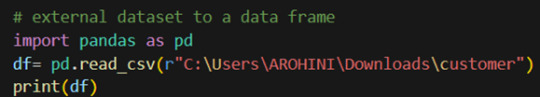
The output of the above code is:

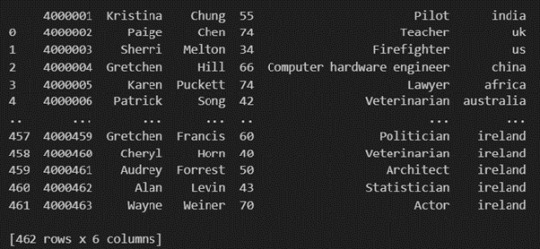
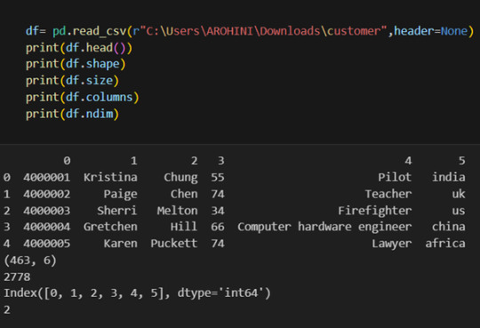
Once your data is loaded into a data frame, you can start exploring it. Pandas offers numerous methods and attributes for getting insights into your data. Here are a few examples:

df.head(): View the first few rows of the DataFrame.

df.tail(): View the last few rows of the DataFrame.

http://df.info(): Get a concise summary of the DataFrame, including data types and missing values.

df.describe(): Generate descriptive statistics for numerical columns.

df.shape: Get the dimensions of the DataFrame (rows, columns).

df.columns: Access the column labels of the DataFrame.

df.dtypes: Get the data types of each column.

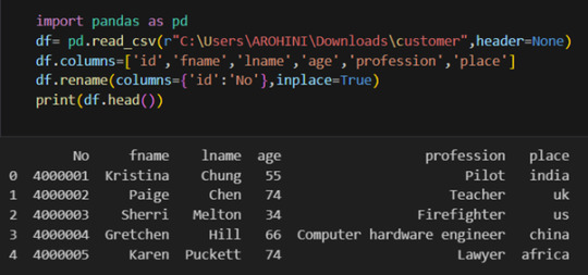
In data analysis, it is essential to do data cleaning. Pandas provide powerful tools for handling missing data, removing duplicates, and transforming data. Some common data-cleaning tasks include:

Handling missing values using methods like df.dropna() or df.fillna().

Removing duplicate rows with df.drop_duplicates().

Data type conversion using df.astype().

Renaming columns with df.rename().

Pandas excels in data manipulation tasks such as selecting subsets of data, filtering rows, and creating new columns. Here are a few examples:

Selecting columns: df[‘column_name’] or df[[‘column1’, ‘column2’]].

Filtering rows based on conditions: df[df[‘column’] > value].

Sorting data: df.sort_values(by=’column’).

Grouping data: df.groupby(‘column’).mean().

With data cleaned and prepared, you can use Pandas to perform various analyses. Whether you’re computing statistics, performing exploratory data analysis, or building predictive models, Pandas provides the tools you need. Additionally, Pandas integrates seamlessly with other libraries such as Matplotlib and Seaborn for data visualization

[subashdhoni86]

Dummy Variables & One Hot Encoding

Handling Categorical Variables with One-Hot Encoding in Python

Introduction:

Machine learning models are powerful tools for predicting outcomes based on numerical data. However, real-world datasets often include categorical variables, such as city names, colors, or types of products. Dealing with categorical data in machine learning requires converting them into numerical representations. One common technique to achieve this is one-hot encoding. In this tutorial, we will explore how to use pandas and scikit-learn libraries in Python to perform one-hot encoding and avoid the dummy variable trap.

1. Understanding Categorical Variables and One-Hot Encoding:

Categorical variables are those that represent categories or groups, but they lack a numerical ordering or scale. Simple label encoding assigns numeric values to categories, but this can lead to incorrect model interpretations. One-hot encoding, on the other hand, creates binary columns for each category, representing their presence or absence in the original data.

2. Using pandas for One-Hot Encoding:

To demonstrate the process, let's consider a dataset containing information about home prices in different towns.

import pandas as pd

# Assuming you have already loaded the data

df = pd.read_csv("homeprices.csv")

print(df.head())

The dataset looks like this:

       town area  price

0 monroe township 2600 550000

1 monroe township 3000 565000

2 monroe township 3200 610000

3 monroe township 3600 680000

4 monroe township 4000 725000

Now, we will use `pd.get_dummies` to perform one-hot encoding for the 'town' column:

dummies = pd.get_dummies(df['town'])

merged = pd.concat([df, dummies], axis='columns')

final = merged.drop(['town', 'west windsor'], axis='columns')

print(final.head())

The resulting DataFrame will be:

  area  price monroe township robinsville

0 2600 550000        1      0

1 3000 565000        1      0

2 3200 610000        1      0

3 3600 680000        1      0

4 4000 725000        1      0

3. Dealing with the Dummy Variable Trap:

The dummy variable trap occurs when there is perfect multicollinearity among the encoded variables. To avoid this, we drop one of the encoded columns. However, scikit-learn's `OneHotEncoder` automatically handles the dummy variable trap. Still, it's good practice to handle it manually.

# Manually handle dummy variable trap

final = final.drop(['west windsor'], axis='columns')

print(final.head())

The updated DataFrame after dropping the 'west windsor' column will be:

  area  price monroe township robinsville

0 2600 550000        1      0

1 3000 565000        1      0

2 3200 610000        1      0

3 3600 680000        1      0

4 4000 725000        1      0

4. Using sklearn's OneHotEncoder:

Alternatively, we can use scikit-learn's `OneHotEncoder` to handle one-hot encoding:

from sklearn.preprocessing import OneHotEncoder

from sklearn.compose import ColumnTransformer

# Assuming 'df' is loaded with town names already label encoded

X = df[['town', 'area']].values

y = df['price'].values

# Specify the column(s) to one-hot encode

ct = ColumnTransformer([('town', OneHotEncoder(), [0])], remainder='passthrough')

X = ct.fit_transform(X)

# Remove one of the encoded columns to avoid the trap

X = X[:, 1:]

5. Building a Linear Regression Model:

Finally, we build a linear regression model using the one-hot encoded data:

from sklearn.linear_model import LinearRegression

model = LinearRegression()

model.fit(X, y)

# Predicting home prices for new samples

sample_1 = [[0, 1, 3400]] 

sample_2 = [[1, 0, 2800]] 

Conclusion:

One-hot encoding is a valuable technique to handle categorical variables in machine learning models. It converts categorical data into a numerical format, enabling the use of these variables in various algorithms. By understanding the dummy variable trap and appropriately encoding the data, we can build accurate predictive models. In this tutorial, we explored how to perform one-hot encoding using both pandas and scikit-learn libraries, providing clear examples and code snippets for easy implementation.

@talentserve

[analysisbyzee]

Classification Decision Tree for Heart Attack Analysis

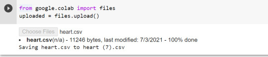
Primarily, the required dataset is loaded. Here, I have uploaded the dataset available at Kaggle.com in the csv format.

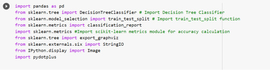
All python libraries need to be loaded that are required in creation for a classification decision tree. Following are the libraries that are necessary to import:

The following code is used to load the dataset. read_csv() function is used to load the dataset.

column_names = ['age','sex','chest pain','resting blood pressure','cholestrol','fasting blood sugar','resting ecg','max heart rate','excercise included','old peak','slp','caa','THALL','output']

data= pd.read_csv("heart.csv",header=None,names=column_names)

data = data.iloc[1: , :] # removes the first row of dataframe

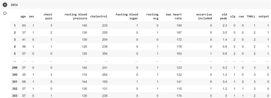
Now, we divide the columns in the dataset as dependent or independent variables. The output variable is selected as target variable for heart disease prediction system. The dataset contains 13 feature variables and 1 target variable.

feature_cols = ['age','sex','chest pain','chest pain','resting blood pressure','cholestrol','fasting blood sugar','resting ecg','max heart rate','excercise included','old peak','slp','caa','THALL']

pred = data[feature_cols] # Features

tar = data.output # Target variable

Now, dataset is divided into a training set and a test set. This can be achieved by using train_test_split() function. The size ratio is set as 60% for the training sample and 40% for the test sample.

pred_train, pred_test, tar_train, tar_test = train_test_split(X, y, test_size=0.4, random_state=1)

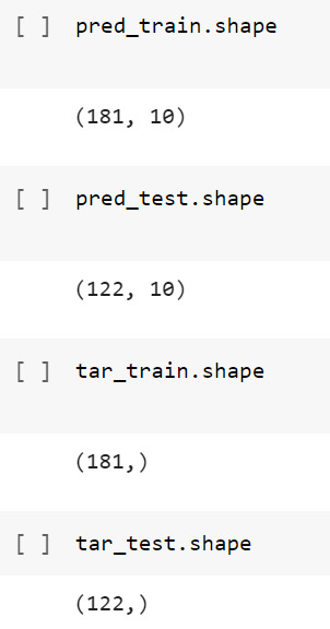
Using the shape function, we observe that the training sample has 181 observations (nearly 60% of the original sample) and 10 explanatory variables whereas the test sample contains 122 observations(nearly 40 % of the original sample) and 10 explanatory variables.

Now, we need to create an object claf_mod to initialize the decision tree classifer. The model is then trained using the fit function which takes training features and training target variables as arguments.

# To create an object of Decision Tree classifer

claf_mod = DecisionTreeClassifier()

# Train the model

claf_mod = claf_mod.fit(pred_train,tar_train)

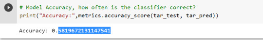
To check the accuracy of the model, we use the accuracy_score function of metrics library. Our model has a classification rate of 58.19 %. Therefore, we can say that our model has good accuracy for finding out a person has a heart attack.

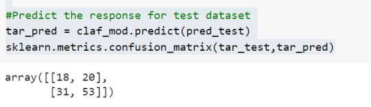
To find out the correct and incorrect classification of decision tree, we use the confusion matrix function. Our model predicted 18 true negatives for having a heart disease and 53 true positives for having a heart attack. The model also predicted 31 false negatives and 20 false positives for having a heart attack.

To display the decision tree we use export_graphviz function. The resultant graph is unpruned.

dot_data = StringIO()

export_graphviz(claf_mod, out_file=dot_data,

filled=True, rounded=True,

special_characters=True,class_names=['0','1'])

graph = pydotplus.graph_from_dot_data(dot_data.getvalue())

graph.write_png('heart attack.png')

Image(graph.create_png())

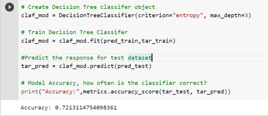
To get a prune graph, we changed the criterion as entropy and initialized the object again. The maximum depth of the tree is set as 3 to avoid overfitting.

# Create Decision Tree classifer object

claf_mod = DecisionTreeClassifier(criterion="entropy", max_depth=3)

# Train Decision Tree Classifer

claf_mod = claf_mod.fit(pred_train,tar_train)

#Predict the response for test dataset

tar_pred = claf_mod.predict(pred_test)

By optimizing the performance, the classification rate of the model increased to 72.13%.

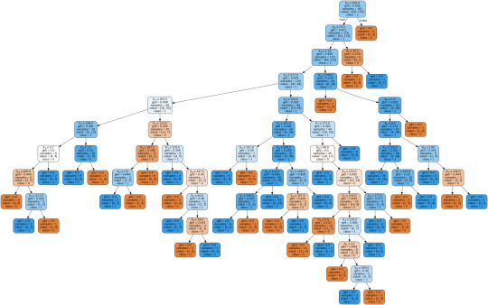
By passing the object again into export_graphviz function, we obtain the prune graph.

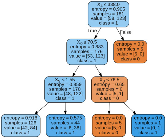
From the above graph, we can infer that :

1) individuals having cholesterol less than 338 mg/dl, age less than or equal to 70.5 years, and whose previous peak was less than or equal to 1.55: 84 of them are more likely to have a heart attack whereas 42 of them will less likely to have a heart attack.

2) individuals having cholesterol less than 338 mg/dl, age less than or equal to 70.5 years, and whose previous peak was more than 1.55: 6 of them will less likely to have a heart attack whereas 38 of them are more likely to have a heart attack.

3) individuals having cholesterol less than 338 mg/dl and age less than or equal to 76.5 years: are less likely to have a heart attack

4) individuals having cholesterol less than 338 mg/dl and age more than 76.5 years: are more likely to have a heart attack

5) individuals having cholesterol more than 338 mg/dl : are less likely to have a heart attack

The Whole Code:

from google.colab import files uploaded = files.upload()

import pandas as pd from sklearn.tree import DecisionTreeClassifier # Import Decision Tree Classifier from sklearn.model_selection import train_test_split # Import train_test_split function from sklearn.metrics import classification_report import sklearn.metrics #Import scikit-learn metrics module for accuracy calculation from sklearn.tree import export_graphviz from sklearn.externals.six import StringIO from IPython.display import Image import pydotplus

column_names = ['age','sex','chest pain','resting blood pressure','cholestrol','fasting blood sugar','resting ecg','max heart rate','excercise included','old peak','slp','caa','THALL','output'] data= pd.read_csv("heart.csv",header=None,names=column_names) data = data.iloc[1: , :] # removes the first row of dataframe (In this case, ) #split dataset in features and target variable feature_cols = ['age','sex','chest pain','chest pain','resting blood pressure','cholestrol','fasting blood sugar','resting ecg','max heart rate','excercise included','old peak','slp','caa','THALL'] pred = data[feature_cols] # Features tar = data.output # Target variable pred_train, pred_test, tar_train, tar_test = train_test_split(X, y, test_size=0.4, random_state=1) # 60% training and 40% test pred_train.shape pred_test.shape tar_train.shape tar_test.shape

# To create an object of Decision Tree classifer claf_mod = DecisionTreeClassifier() # Train the model claf_mod = claf_mod.fit(pred_train,tar_train) #Predict the response for test dataset tar_pred = claf_mod.predict(pred_test) sklearn.metrics.confusion_matrix(tar_test,tar_pred) # Model Accuracy, how often is the classifier correct? print("Accuracy:",metrics.accuracy_score(tar_test, tar_pred)) dot_data = StringIO() export_graphviz(claf_mod, out_file=dot_data, filled=True, rounded=True, special_characters=True,class_names=['0','1']) graph = pydotplus.graph_from_dot_data(dot_data.getvalue()) graph.write_png('heart attack.png') Image(graph.create_png())

# Create Decision Tree classifer object claf_mod = DecisionTreeClassifier(criterion="entropy", max_depth=3) # Train Decision Tree Classifer claf_mod = claf_mod.fit(pred_train,tar_train) #Predict the response for test dataset tar_pred = claf_mod.predict(pred_test) # Model Accuracy, how often is the classifier correct? print("Accuracy:",metrics.accuracy_score(tar_test, tar_pred)) from sklearn.externals.six import StringIO from IPython.display import Image from sklearn.tree import export_graphviz import pydotplus dot_data = StringIO() export_graphviz(claf_mod, out_file=dot_data, filled=True, rounded=True, special_characters=True, class_names=['0','1']) graph = pydotplus.graph_from_dot_data(dot_data.getvalue()) graph.write_png('improved heart attack.png') Image(graph.create_png())

[pabloatech]

Week 3:

I put here the script, the results and its description:

PYTHON:

Created on Thu May 22 14:21:21 2025

@author: Pablo """

libraries/packages

import pandas import numpy

read the csv table with pandas:

data = pandas.read_csv('C:/Users/zop2si/Documents/Statistic_tests/nesarc_pds.csv', low_memory=False)

show the dimensions of the data frame:

print() print ("length of the dataframe (number of rows): ", len(data)) #number of observations (rows) print ("Number of columns of the dataframe: ", len(data.columns)) # number of variables (columns)

variables:

variable related to the background of the interviewed people (SES: socioeconomic status):

biological/adopted parents got divorced or stop living together before respondant was 18

data['S1Q2D'] = pandas.to_numeric(data['S1Q2D'], errors='coerce')

variable related to alcohol consumption

HOW OFTEN DRANK ENOUGH TO FEEL INTOXICATED IN LAST 12 MONTHS

data['S2AQ10'] = pandas.to_numeric(data['S2AQ10'], errors='coerce')

variable related to the major depression (low mood I)

EVER HAD 2-WEEK PERIOD WHEN FELT SAD, BLUE, DEPRESSED, OR DOWN MOST OF TIME

data['S4AQ1'] = pandas.to_numeric(data['S4AQ1'], errors='coerce')

Choice of thee variables to display its frequency tables:

string_01 = """ Biological/adopted parents got divorced or stop living together before respondant was 18: 1: yes 2: no 9: unknown -> deleted from the analysis blank: unknown """

string_02 = """ HOW OFTEN DRANK ENOUGH TO FEEL INTOXICATED IN LAST 12 MONTHS

Every day

Nearly every day

3 to 4 times a week

2 times a week

Once a week

2 to 3 times a month

Once a month

7 to 11 times in the last year

3 to 6 times in the last year

1 or 2 times in the last year

Never in the last year

Unknown -> deleted from the analysis BL. NA, former drinker or lifetime abstainer """

string_02b = """ HOW MANY DAYS DRANK ENOUGH TO FEEL INTOXICATED IN THE LAST 12 MONTHS:

"""

string_03 = """ EVER HAD 2-WEEK PERIOD WHEN FELT SAD, BLUE, DEPRESSED, OR DOWN MOST OF TIME:

Yes

No

Unknown -> deleted from the analysis """

replace unknown values for NaN and remove blanks

data['S1Q2D']=data['S1Q2D'].replace(9, numpy.nan) data['S2AQ10']=data['S2AQ10'].replace(99, numpy.nan) data['S4AQ1']=data['S4AQ1'].replace(9, numpy.nan)

create a subset to know how it works

sub1 = data[['S1Q2D','S2AQ10','S4AQ1']]

create a recode for yearly intoxications:

recode1 = {1:365, 2:313, 3:208, 4:104, 5:52, 6:36, 7:12, 8:11, 9:6, 10:2, 11:0} sub1['Yearly_intoxications'] = sub1['S2AQ10'].map(recode1)

create the tables:

print() c1 = data['S1Q2D'].value_counts(sort=True) # absolute counts

print (c1)

print(string_01) p1 = data['S1Q2D'].value_counts(sort=False, normalize=True) # percentage counts print (p1)

c2 = sub1['Yearly_intoxications'].value_counts(sort=False) # absolute counts

print (c2)

print(string_02b) p2 = sub1['Yearly_intoxications'].value_counts(sort=True, normalize=True) # percentage counts print (p2) print()

c3 = data['S4AQ1'].value_counts(sort=False) # absolute counts

print (c3)

print(string_03) p3 = data['S4AQ1'].value_counts(sort=True, normalize=True) # percentage counts print (p3)

RESULTS:

Biological/adopted parents got divorced or stop living together before respondant was 18: 1: yes 2: no 9: unknown -> deleted from the analysis blank: unknown

2.0 0.814015 1.0 0.185985 Name: S1Q2D, dtype: float64

HOW MANY DAYS DRANK ENOUGH TO FEEL INTOXICATED IN THE LAST 12 MONTHS:

0.0 0.651911 2.0 0.162118 6.0 0.063187 12.0 0.033725 11.0 0.022471 36.0 0.020153 52.0 0.019068 104.0 0.010170 208.0 0.006880 365.0 0.006244 313.0 0.004075 Name: Yearly_intoxications, dtype: float64

EVER HAD 2-WEEK PERIOD WHEN FELT SAD, BLUE, DEPRESSED, OR DOWN MOST OF TIME:

Yes

No

Unknown -> deleted from the analysis

2.0 0.697045 1.0 0.302955 Name: S4AQ1, dtype: float64

Description:

In regard to computing: the unknown answers were substituted by nan and therefore not considered for the analysis. The original responses to the number of yearly intoxications, which were not a direct figure, were transformed by mapping to yield the actual number of yearly intoxications. For doing this, a submodel was also created.

In regard to the content:

The first variable is quite simple: 18,6% of the respondents saw their parents divorcing before they were 18 years old.

The second variable is the number of yearly intoxications. The highest frequency is as expected not a single intoxication in the last 12 months (65,19%). The more the number of intoxications, the smaller the probability, with an only exception: 0,6% got intoxicated every day and 0,4% got intoxicated almost everyday. I would have expected this numbers flipped.

The last variable points a relatively high frequency of people going through periods of sadness: 30,29%. However, it isn´t yet enough to classify all these periods of sadness as low mood or major depression. A further analysis is necessary.

[learning-code-ficusoft]

A Beginner’s Guide to Pandas: Data Manipulation Made Easy

A Beginner’s Guide to Pandas: 

Data Manipulation Made Easy Pandas is one of the most powerful and widely used Python libraries for data manipulation and analysis. 

It simplifies working with structured data, making it an essential tool for anyone in data science, machine learning, or data analysis. 

What is Pandas? 

Pandas is an open-source library that provides data structures and data analysis tools for Python. The core data structures in Pandas are: 

Series: A one-dimensional array-like object that can hold any data type. 

DataFrame: 

A two-dimensional, size-mutable, and potentially heterogeneous tabular data structure with labeled axes (rows and columns).

 Key Features of Pandas: 

Data Cleaning:

 Pandas makes it easy to clean and preprocess data, such as handling missing values, filtering, and transforming data. 

Data Exploration: 

With simple commands, you can explore datasets by calculating statistics, summarizing data, and visualizing distributions.

 Data Manipulation: 

Pandas excels in reshaping, merging, and joining datasets, allowing for complex transformations with minimal code. 

Commonly Used Pandas Functions: 

read_csv(): Loads data from a CSV file into a DataFrame. 

dropna(): Removes missing values from the dataset. 

groupby(): Groups data by a specific column and performs aggregate functions. 

merge(): Combines two DataFrames based on common columns or indices. 

Why Learn Pandas? 

Efficiency: 

Pandas is highly optimized for performance and handles large datasets with ease. 

Versatility:

 It integrates well with other libraries like NumPy, Matplotlib, and Scikit-learn, providing a seamless workflow for data analysis and machine learning projects.

 Ease of Use: 

The syntax is intuitive, and the library is well-documented, making it easy for beginners to get started. 

conclusion

 mastering Pandas opens the door to efficient data manipulation and analysis, making it an essential tool for anyone working with data in Python. 

Whether you are cleaning data, analyzing trends, or preparing datasets for machine learning, Pandas will simplify the process.