#pandas how to remove a column

[codewithnazam]

How to Drop a Column in Python: Simplifying Data Manipulation

Dive into our latest post on 'Drop Column Python' and master the art of efficiently removing DataFrame columns in Python! Perfect for data analysts and Python enthusiasts. #PythonDataFrame #DataCleaning #PandasTutorial 🐍🔍

Hello, Python enthusiasts and data analysts! Today, we’re tackling a vital topic in data manipulation using Python – how to effectively use the Drop Column Python method. Whether you’re a seasoned programmer or just starting out, understanding this technique is crucial in data preprocessing and analysis. In this post, we’ll delve into the practical use of the drop() function, specifically…

[squish36-writes-and-draws]

Import Cygnus Oscuro

Summary: Creative Writing Final. It's a fedex humans are space orcs au. They're forced to be in the proximity of one another and it's fun for everyone except for those directly involved.

Word count : 5244

TW: one (1) swear word, auton (robot) racism including an in-universe slur (thanks, Fitz), absolutely incomprehensible worldbuilding (thanks, Squish)

Taglist (lmk if you want to be added/removed!): @stellar-lune @faggot-friday @kamikothe1and0nly @nyxpixels @florida-preposterously @poppinspop @uni-seahorse-572 @solreefs @i-loved-while-i-lied @rusted-phone-calls @when-wax-wings-melt @good-old-fashioned-lover-boy7 @dexter-dizzknees @abubble125 @hi-imgrapes @callum-hunt-is-bisexual @callas-pancake-tree @hi-my-name-is-awesome @katniss-elizabeth-chase @arson-anarchy-death @dizzeners @thefoxysnake @olivedumdum @loveution

On Ao3 or below the cut!

Bonus worldbuilding / q&a / suffering because I doubt any of this makes sense

    import pandas as pd

    import numpy as np

    import matplotlib.pyplot as plt

    from sklearn import datasets, model_selection, metrics

    from sklearn.model_selection import train_test_split, cross_val_score

    from sklearn.preprocessing import *

    from sklearn.neighbors import KNeighborsClassifier

    from sklearn.metrics import *

    “Once again, what do you mean by Eifelia? The planet itself or the system as a whole, including its moons?” Sophie asks, staring out the window at the receding planetary surface as their spaceship affectionately called the ‘Cygnus Oscuro’ lifts off the ground. 

    “Eifelia has only one confirmed inhabited moon, Batyrbai. Your home planet of Datson is the only satellite in the Telychian system to have more than one moon that is suitable for habitation. Supplies were acquired at the port of Darriwilian, located at 25.78, -80.21, on the planet of Eifelia itself,” Dex replies, reading off the coordinates from the corner of xor vision. 

    It’s very easy to read off coordinates when xor neural network is constantly searching for information that it thinks will be helpful to xem. It, more often than not, is entirely extraneous information, but it is difficult to discern when, exactly, it will be of assistance. 

    Dex continues, “Five crew members departed in preparation for Eifelia’s cyclical festival of Batyrbai appearing full in the sky from the dark side of the planet. In turn, three crew members embarked.”

    Dex’s fan freezes up. “One of these crew members is human, which hail from Earth, most accurately described as a ‘Death Planet’. It is located in the system of Sol, 40.3 light years away. Take care to avoid any and all possible conflicts.” 

    Sophie fixes Dex an unbelieving look. “They can’t be that bad.”

    Article after article scroll across Dex’s field of vision. “They’ve earned their infamous reputation and most are highly unaware of it. Did you know they have contests to see which one can suffer through the most capsaicin-induced pain? Then, to cool the pain, they consume a drink full of near-impossible-to-digest lactose sugar.”

    “Yeah, and you can bend titanium without even a second thought.”

    “I’m sure a dedicated enough one would figure out how to do that.” 

    Sophie rolls his eyes. “I’ll make sure to tell Keefe not to be an intergalactic space wyrm this week but I don’t think that’s going to be happening any time soon.” 

    Dex’s processor runs the numbers, and Sophie is correct for once. In any other situation, a correct prediction from him would be a thing to praise, but in this particular case, it’s more worrisome for Keefe’s safety.

    stars_df = pd.Dataframe(data=stars.data, columns=stars.feature_names)

    stars_df.iloc[39060]

    name                “Beta Pictoris c”

    distance_ly         60         # light years, 3*10^8 m/s

    yerkes_stellar_class    “A6V”

    mass                4658.44    # Eifelia masses, 4.13*10^24 kg

    orbital_period         197.55     # Eifelia years

    grav_accel         182.470    # m/s^2

    surface_temp        1250       # kelvin

    “Greetings,” Dex’s assigned partner says as Dex slides into the chair next to him. His voice is blanketed with a thick accent Dex’s processor is unable to place, though the circling loading sign in the top corner is certainly trying. Such is the curse of exploring new planets faster than xor updates are able to keep track of them. 

    Today’s mission is expected to make that problem worse, although only slightly.     

    “I’m Fitz,” he says, holding out a hand.    

    “I’m D3x+3r,” Dex replies, not actually pronouncing the numbers like numbers even if they should be pronounced like numbers because they are numbers. The loading wheel is still circling around itself. “Although most people call me Dex because apparently two syllables is too many. I don’t understand it either.” 

    Fitz’s hand falls into his lap. “Nice to meet you, Dex.” He pauses. “Unless you have anything else I’ve forgotten, I think we can probably get going down to the surface so that we can get back sooner than later.” 

    Dex pushes away the loading circle in favor of the small transport ship’s inventory list. “I believe we have everything. If that is a false presumption, the communication link with the Cygnus Oscuro is up and running.” 

    Fitz gently undocks from the Cygnus Oscuro and that’s when Dex’s processor finally decides to provide xem with any information. It’s odd how it’s so proficient with useless information and finally now that it’s relevant, it takes a suspiciously long time. 

    It apparently doesn’t think it’s a major priority to know that xe’s just been sealed into a very small shuttle with a human. No big deal. This is both fine and normal. It’s not like they’re documented to have very short tempers. 

    Now the accent makes sense. Humans have hundreds of different languages, owing to their incredibly diverse geographic distribution. Most other species, including the Eifelians, only exist in small pockets in the corners of their worlds. Humans looked at that and went ‘no, I don’t think I will.’ Any other species is almost immediately recognizable by their accent but humans. They live to be difficult. 

    Even if the accent hadn’t been atrociously obvious in hindsight, the lines streaking across his skin—Blaschko lines, Dex’s processor claims—should have given his heritage away. The even more entertaining part is that most humans don’t even know they have them. 

    Dex’s processor is able to pull up Fitz’s official file without too much difficulty, and that seems like a mostly safe conversation to have instead of stilted silence. “So, how long have you been part of Parallax?” 

    “Well, my parents have worked here since before I was born, so the answer I usually give is, ‘Yes.’ How about you?” 

    “I was built on Gzhelia roughly 250 Eifelia years ago.” Dex pauses, converting this to a unit hopefully a little more familiar to Fitz. “That’s a little more than 4 Earth years.” 

    Fitz’s brows draw together. “Built?”

    Dex’s fan pauses in such a way that it sounds like a sigh as xe pulls back the artificial skin away from xor wrist, revealing the wires twisting underneath. A green fiber optic cable shimmers in the artificial light of the shuttle. 

    “I am aware that I am running on slightly older hardware, but I promise that my software is as updated with the most current Parallax Dataframes an update cycle half an Eifelia year ago could provide. Again, for ease of conversion, that is about three Earth days.”

    “You can stop with that. The conversions. I’ve grown up around more Eifelia time than Earth time.” 

    “I apologize. I was simply trying to prevent any incidental miscommunication before there was an issue. I will refrain from it in the future.” 

    The table of conversions still floats in front of Dex’s vision like a temporary burn-in.    

    Dex and Fitz sit in a silence that even Dex’s emotion identifier that was deprecated two years ago can identify as uncomfortable. Xe really should get around to installing a new one. 

    Fitz is the one to break the silence. “How’d you know I was human? Your little CPU tell you?” 

    Dex nods slowly. “Yes, it did, along with installing several files explaining your species’ customs. I can feel one of them slowing down my SSD flash memory with its sheer size.” 

    “Yeah, yeah, we all get it. Humans are big and loud and dumb and there’s so many of us that you can’t be bothered to learn all of it.” 

    Fitz flicks a half-dozen switches, initiating the landing sequence of the shuttle now that it is within the last thousand kilometers of altitude. The reason that it has to be activated so early is due to Beta Pictoris C’s incredibly high gravitational acceleration, causing the shuttle to have a much higher velocity than if it were under the gravitational influence of most other planets. 

    In other, more numerical terms, gravitational acceleration on Beta Pictoris C at the surface is about 182.970 m/s2, while, for reference, Eifelia’s is 8.011 m/s2. Of course, they are still up in the air, meaning that their orbital radius is slightly larger than the planet’s radius, but that really is not that much of a difference due to the sheer scale of the planet. 

    It’s no wonder Parallax has chosen the two of them for this mission—they’re the most likely to not be crushed under the sheer weight of the surface gravity. Or, more accurately, their own weight due to the increased surface gravity. 

    Fitz touches down gently, one of the very few landings Dex has experienced without involving a significant amount of screaming. 

    “Are you ready to go find one amino acid and then leave?” he asks, standing up. 

    Searching for life on planets like these is, for lack of a better descriptor, a neural-network-numbing process involving taking a few dirt samples while trying to make sure that Dex’s zinc components don’t get instantaneously vaporized, among other problems. 

    A-type stars aren’t even the hottest ones out there, but they’re on the very edge of what is believed to be habitable due to their instability. Their scarcity in the universe also makes it much more unlikely for life to have the opportunity to form around one. 

    It’s nearly inhospitable to every life form currently described, leaving a few carbon-fiber autons to figure out how to sample things on stars-forsaken planets that are literally half the surface temperature of Eifelia’s home star, Telychia. 

    “It would probably be beneficial to don some protective clothing before doing that, even if Beta Pictoris C is nearing aphelion and we have landed on the night side. Do you happen to know if it is tidally locked?”

    “That’s not in your file system?”

    “I regrettably am unable to locate it if it is.” 

    Fitz rolls his eyes, muttering, “Turing incomplete,” under his breath. 

    It takes a few milliseconds for Dex’s processor to provide the context to that statement, and that context is not a flattering one. Its origins lie with both the first human theoretical computer scientist, Alan Turing, and it became popularized due to Earth’s history with artificial intelligence. 

    It’s…not a pleasant history. 

    “Do you believe that infinite memory is possible? Because everything is technically only Turing complete when it is assumed to have infinite amounts of memory, which is impossible to create in the real world. Thus, every device, including this shuttle and your knee replacement is Turing incomplete.

    “Yeah, but at least I can feel emotions.”

    Fitz slides the heat suit’s helmet over his head, obscuring his face.

    “Most of your emotions are induced by shifts in hormonal signals. The Floians don’t have hormones. Does that mean that they too are artificial because they do not experience emotions in the same way that you do?” 

    Fitz opens the shuttle door, pressing himself against the wall to avoid being blown away by both the swirling, windy atmosphere blowing dust into all of the delicate machinery of the shuttle and the zeroth law of thermodynamics. 

    Dex’s fan immediately kicks into its highest gear, and it will stay there as long as the door remains open, barring some catastrophic, friction-related disaster. 

    “The Floians had to figure out how to evolve on their own. That should be a reasonable enough distinction for you.”

    “That implies that genetically modified organisms don’t count as organisms. And then, most autons learn via a reinforcement algorithm that mimics how evolution works in order to train a neural network. That’s the thing that I have making decisions in my ‘little CPU’ and its trillion transistors. How many neurons do you have again?”

    Fitz steps out into the outside, his suit making him look like a large orange nebula. Hopefully the door doesn’t decide to close with its own artificial consciousness like last time. That was not a fun time. 

    “Why do you ask when you could just search through your files? I’m sure it’s in there.” 

    “The answer was 135 billion,” Dex says flatly. That would be a more relevant description if xe was able to inflect xor speech more, but xe has found the setting to make xor voice a specific frequency and uses it a touch more than xe probably should. 

    Fitz turns back to Dex. “What are you doing? The sooner we get these samples into your file system, the sooner I stop looking like the stay puft marshmallow man.”

    Dex smiles as the image flashes across xor vision. Xe follows Fitz down the ramp, revealing the expected vast desertlike landscape of Beta Pictoris C.

    It’s significantly too hot for water to remain liquid but—there’s something odd about the erosion patterns. Those might not just be wind erosion. Xe downloaded a whole library of algorithms a couple of months ago. 

    Ignoring Fitz’s demands to know where xe’s going, Dex approaches one of the striated, gray rock formations. 

    url = 'https://docs.google.com/spreadsheets/d/e/2PACX-1vTCZgoegOH a49SFXYU-ZZTdCkgTp0sn&single=true&output=csv'

    rocks_df = pd.read_csv(url)

    features = rocks[["depth", "width", "mohs_hardness"]]

    label = stars_df["class"]

    X_train, X_test, y_train, y_test = model_selection.train_test_split(features, label, test_size = 0.2, random_state = 42)

    model = KNearestNeighbor(n_neighbors = 53)

    model.fit(X_train, y_train)

    new_rock = pd.Dataframe([7,4,6.5])

    pred = model.predict(new_rock)

    A smile blossoms across Dex’s face. “We’ve got liquid erosion. It’s slightly less viscous than water, but liquid erosion nonetheless.” 

    Fitz stares at xem, waiting for an explanation that takes a long time to get there. 

    “I’m going to have to run some simulations on the ship because I don’t have enough RAM for the kind of resolution I want, but there’s potential that there used to be water here, and I’m sure you’re aware of how water and life are synonymous. Most of the time.” 

    Dex carefully scrapes off a corner of the ashy sandstone column for further study because xe, quite unfortunately, doesn’t have a built-in mass spectrometer. It’s also generally good practice to collect samples. 

    Another aspect of good practice is to look at more than one rock before drawing conclusions about an entire planet. 

    Dex traces into the dirt a simple sketch of Fitz in his marshmallow suit. He’s lucky to have all of his appendages attached, let alone proportional. Dex then takes a sample of the dirt. The mixing helps to paint a better picture of what the sand is like, rather than just the solar-radiation-exposed topsoil. 

    Suddenly, Fitz swears, pointing at something in the vial. That something is a little creature wiggling its way around the glass. 

    Dex nearly drops it, which would have been a less than ideal decision, as xe tries to find the little guy who is desperately trying to not be seen. 

    The little guy is a fairly standard arthropod-style body plan, with an exoskeleton, a number of legs that is larger than 2 and smaller than the number required for ‘burn it alive’ algorithms to kick in. So somewhere in the 6,8,10 range is probably pretty reasonable. 

    Although, to be fair, even numbers are more of a guideline than anything else. Once again, Earth is an exception to the rule with a three legged fish down in some of the deepest parts of its oceans. Also echinoderms with their five-fold radial symmetry. 

    “You, uh, might want to put him down,” Fitz suggests. “You don’t want to be charged with kidnapping should that little bug guy who I’m now going to be naming Fred turn out to have a consciousness.”

    Humans’ inclination to name creatures that have no way of communicating with them is a fairly large section in their file overview. It seems as though this can even occur with inanimate objects, which just links to a page advertising a pet rock, whatever that’s supposed to mean. 

    Dex pours the vial back onto the ground and attempts to take another sample without kidnapping another Fred. 

    Is that how human naming goes? Does it really matter? 

    The only reason this is a question is probably because It feels like all of Dex’s wires are currently being poached in the water designed to cool them. 

    There’s another one in the next vial. And the next. It’s almost like spontaneous generation but, like, not yet disproven by putting meat in a jar and covering it so maggots don’t get laid on it. 

    Yeah, that’s literally what the humans decided to do. Specifically one named Francesco Redi. Seems like a waste of calories for a species who needs to eat a lot of them to support their endothermic metabolisms. At least they figured it out in the end. 

    The fourth attempt seems to be safe as Dex only fills the vial halfway and shakes it extensively to avoid accidental kidnapping. Now the only possible complication could be microscopic creatures, but that’s past the point of reasonable care. 

    Fitz spends another few minutes gallivanting around, likely wandering around for more interesting samples, even if the entire report is already writing itself in the back of Dex’s processor. 

    He returns with a half dozen more samples of varying mineral compositions which get stored in his marshmallow suit’s pockets. “I saw another guy. Sorry I couldn’t get a picture, but he kind of looked like a scorpion. If you know what those are.”

    Dex nods, projecting a picture of one onto the first rock ledge just to prove that xe has image files stored in xor drive. 

    “Yeah, he looked kind of like that.”

    Dex switches the picture to a different one, one that isn’t necessarily a true scorpion. That doesn’t stop Eurypterus from colloquially being called a sea scorpion. It also doesn’t stop them from being extinct on Earth for around 252 million of its own years. 

    Fitz repeats, louder this time, “Yeah, he looked kind of like that.” 

    Fitz’s new best friend the Beta Pictoris C scorpion, who notably has yet to be blessed with a name, hops up onto the rock ledge, and it’s remarkable how similar they look, albeit the hologram being significantly larger. Blue swirls across its hardened exterior, and its pincers look like they’re very ready to reduce the number of fingers Dex has. 

    A warning light flicks on in the corner of Dex’s vision, cutting off access to xor files. 

    “We should probably be getting back to the ship. I have the coordinates of our landing point so that a larger, more prepared team can conduct a more detailed study. And before you begin to state that we are that team, if I am to stay out here for much longer, I will probably end up shutting down, and that is a burden I would rather not impose upon you.”

    It’s kind of odd how Dex’s vision is able to start flickering as xor processor threatens to have enough for the day. One would think it would work the same as when it gets too cold, but no. One second, xe’s completely fine and the next, xe’s restarting after eighteen hours trapped in an avalanche. 

    This is a normal experience. It’s not Dex’s first time, and most other autons xe has communicated with have had similar ones. It’s a risk associated with the job, and xor data won’t be lost in anaerobic environments the same way that data in an biologically-designed brain will. 

    Unless that brain belongs to an obligate or facultative anaerobe, but the vast majority of intelligent species do require some form of a gas to function. Many use oxygen, but carbon dioxide, methane, hydrogen, and carbon monoxide are fairly common as well. 

    Dex and Fitz make their way back into the spaceship and make absolutely certain that the hatch is sealed before peeling off their marshmallow suits. Dex’s blinking temperature warning sign disappears, but xor fan still remains running at full speed. 

    Fitz collapses into the pilot’s chair, sweat streaking down his brow, and barely waits for Dex to sit down beside him before lifting off. 

    They once again sit in an uncomfortable silence, punctuated only by the sounds of Fitz flipping various switches on the shuttle’s control panels. 

    Dex makes half a note that xe should learn how to fly a ship at some point, although Sophie would rapidly abuse that particular ability. 

    Once xe’s back aboard the Cygnus Oscuro, xe locates the mass spectrometer in order to analyze the samples before Fitz starts telling everyone about the larger portion of their discovery, because then xe’s going to have to answer other people’s questions instead of xor own.

    url = ‘https://docs.google.com/spreadsheets/d/16lsnIQaP37r682gKuz CZp-YqLgCis-Ln4PSaDEpiAjw/edit#gid=0’

    mass_spec = pd.read_csv(url) 

    compounds = []

    for i in range(mass_spec.size()): 

        id = identify(mass_spec[i]) 

        compounds += id 

     It turns out to absolutely no one’s surprise that liquid water doesn’t exist inside of the rock samples, but tricobalt tetraoxide, Co3O4, is in there, and it is a liquid at the planet’s surface temperature. It’s certainly a choice for an electron donor, and it’s kind of a wonder the entire planet isn’t bright blue with the Cobalt (ii) ions. 

    Dex isn’t surprised to find out that by the time xe’s had enough time with the samples that the entire ship knows about the little arthropod that was found, even if they aren’t formally related to the Earthen order of arthropoda Fitz is comparing it to. 

    They look similar. It’s close enough. 

    What Dex is surprised to find is that everyone wants a tour to see them despite the fact that the vast majority of the crew would acquire heat stroke almost instantaneously. This is xor thirty-sixth mission to actually go down onto a planet for the first time—autons are cheaper to replace than biological organisms—and this is by far the biggest response to a new species. 

    It’s odd. Xe doesn’t like it. 

    Dex’s neural network wants to blame it on Fitz, and there really isn’t any data to contradict that particular hypothesis. It also makes it a very difficult hypothesis to test, which makes it significantly less useful as a hypothesis. 

    On the other hand, a useful hypothesis would be one relating to the actual little alien creatures that for some reason are able to live on a planet that’s more similar to a furnace than a habitable landscape. 

    And so, against all logical reasons surrounding the temperature of a planet known to be at least twice the temperature of the hottest previously confirmed life forms. Of course it’s on Earth. Hydrothermal vents don’t look like a place where organisms could live, and then they’re just down there chilling. That’s probably not the best choice of a descriptor. 

    When in doubt, the answer is more often than not ‘Earth is a weird planet.’ 

    The journey back down to the surface with Fitz passes with significantly less fanfare than the first, the beeping of the ship being obnoxiously loud in the deafening silence. 

    They touch down, Fitz not taking as much care as last time with making sure the landing has as little of a change in momentum as possible, which is to say that it’s nowhere near the gentle landing of the first trip. 

    Fitz leans back and sighs. “Do you have any commentary you’d like to provide or are you ready to go and collect data so we can finish our reports on this planet?”

    “I mean, I’m always collecting data, even if it's only a live feed of my precise coordinates getting thrown into a plaintext file never to be seen again, so the answer is closest to both of the above.” 

    That does not seem to be the answer Fitz wants as he takes one of his bags of human snacks—potato chips, according to what’s printed on the yellow label—and throws it into the garbage can in the corner. 

    “Wow.” Dex’s visual apertures widen. “I didn’t realize that throwing projectiles with accuracy was a human skill. I’ll make sure to add that to my files, as well as to the main system.”

    Fitz’s eyes flash, his features drawing into hard lines. “Are you physically incapable of not being condescending? I get it. I’m a human. I’m from a death planet. Humans are weirder than fucking dark energy. It doesn’t require that many comments about it to get your point across!”

    Dex pauses, letting xor neural network fully process Fitz’s statements before replying, “I don’t understand where I was being condescending.”

    “You just did it two sentences ago!”

    “I did not do anything two sentences ago. It was genuinely quite interesting how your species has evolved to throw objects with accuracy, even ones with high surface area to volume ratios such as that bag of chips, because it is not something that has been documented in any other intelligent species.” 

    “Oh, please. It’s a basic skill.”

    “Do remember that your species evolved in part to bring down large prey such as Mammuthus primigenius. Throwing spears at a wooly mammoth directly led to that ability being rewarded with a higher rate of nutrients, and thus resulted in the following generations being more able to throw spears as well.”

    “You know all of that but you didn’t figure out that throwing things is pathetically easy? Your little auton brain isn’t very good at drawing conclusions from data you have, is it?”

    “It is simply something I did not have cause to consider before now, though I do recognize that it would have been quite easy to identify without the inciting event.”

    “And you’ve also said that you have a very large file on humans. Most of our games are based around the concept of throwing a ball. Was that not enough information to extrapolate that maybe we’re good at it?”

    “Games of chance are common in many species. It follows that this could simply be a manifestation of that desire in humans, so games like your ‘basketball’ or ‘baseball’ do not provide sufficient evidence to draw conclusions such as the ones you’re suggesting.”

    Fitz rolls his eyes. “Why do I even bother? It’s not like you’re going to change your mind. You don’t have a mind to change.”

    Dex wants to explain that xor neural network is actually changing its dependence on its individual notes on a regular basis, but that doesn’t seem to be advantageous in this particular context.

    Fitz rolls his eyes, muttering in what is likely his native tongue—one which Dex has not downloaded the translation file of—as he gets into the marshmallow suit once again. 

    They go out, describe a half dozen new arthropod-esque species, each with more legs than the last, and return with more samples with as few words as possible. But nothing is ever allowed to be simple. 

    The hatch on the shuttle has decided today that leaving itself open in the blistering heat is not something it likes to do, and while Fitz and Dex are distracted, it shuts its doors. 

    In turn, it opens the floodgates for Dex to learn some new fun human swear words when Fitz notices what’s happened. 

    “No reason to worry,” Dex says, making xor way through the sand to open up the back emergency panel that exists for exactly this reason. 

    “Uh, I left the keys in there. There’s very much a reason to worry.”

    “And I’ve got admin privileges. It’s fine. Go back to looking for the next beetle you’re going to call your son.”

    “Don’t be rude to Benny like that. He’s not that replaceable.”

home@Cygnus-shuttle-3:~$sudo su

home@Cygnus-shuttle-3:~$******

root@Cygnus-shuttle-3:~$ufw disable 

    There’s no particular reason why the firewall sometimes decides to make the hatch close, and this is enough of a solution for Dex to not go searching for an answer. 

    As the door begins to open again, Fitz asks, “So, what’s the password?”

    “I’m the password.”

    “Yes, yes, I understand that you’re helpful. Now, what’s the password if this were to happen again and you aren’t around?”

    “I’m the password. It’s literally just my name. D3x+3r. It’s got an uppercase character, lowercase character, number, and a special character. My friend Sophie thought he was hilarious when he heard it, so now it’s my password for everything. Don’t tell anyone.”

    “I won’t. I don’t even know where the special characters are even if I wanted to.”

    “The ‘t’ is replaced with a plus. The ‘e’s are fairly obviously transliterated to ‘3’s. There’s nothing fancy going on here.”

    Fitz turns to walk away but stops himself. “The name Sophie feels a little familiar. Does he by any chance know a Keefe?”

    “Yes, actually. The two of them dated for a while. Although I’m not sure if that should be in the past tense. I stopped asking for updates a while ago.” 

    Fitz laughs. “Stars, I wish I could figure out how to do that. I’ve never escaped from them.”

    “Just kind of stare blankly into the distance and people will stop wanting to tell you things. They’re usually doing it because they want compliments on whatever it is they’re telling you, and by depriving them of that, they stop wanting to do that.”

    “Are you sure you’re an auton?”

    Now it’s Dex’s turn to laugh, a sound xe was very much not designed to make, so it sounds more like an out of tune record skipping. “Yeah, I think so. I’ve walked into too many door frames to have gone this long without getting a contusion, which is another thing your species doesn’t particularly care about getting.”

    ��Case in point: I found one on my leg yesterday and I have no idea how I got it. It’s already green and I’m not sure how I hadn’t noticed it before. I guess that’s what I get for being from a death world.”

    Dex gestures widely to the rolling desert around xem. “I think Earth’s death world status may be a bit outdated. If this isn’t a death world, I don’t know what is, and, by comparison, I’m pretty sure Earth is an absolute paradise. You didn’t have to evolve to use tricobalt tetraoxide as an electron donor.”

    “We’ve also had five mass extinctions,” Fitz interjects. 

    “So has everybody else, including the Datsonians, even if their government would rather not admit that out loud. You’re not special.”

    Fitz snaps his fingers inside of the marshmallow suit, which does not work well with the thick padding of the gloves. “And that’s exactly what I wanted you to admit.”

    “Is that why you volunteered to come back down here?”

    “That was mostly a decision based on Parallax’s inability to find another poor sap that would be willing and able to come down here.”

    “Wouldn’t it be really funny if they send a Gzhelian in your place?”

    Fitz smiles, the sound of the air conditioners they use onboard the Cygnus Oscuro at a nice, toasty 200 kelvin having kept him from sleeping for nearly as many hours as Dex has wanted to disconnect xor audio input. 

    A beat of silence stretches in the space between them, but for the first time it isn’t immensely uncomfortable. 

    “We should probably be getting back inside the shuttle before it decides to close again,” Dex says, even if it would be very entertaining if they stood outside long enough for it to grow its own intelligence again. 

    After all, that’s kind of how xe got here. Xe’s going to get replaced by a shuttle door within the next couple of Eifelia years. 

    Xe’ll probably get assigned to, like, repairing the Cygnus Oscuro in all of the places the non-auton mechanics are unable to go, but at least xe’ll have discovered a wondrous new world before that happens. 

    while True: 

        # avoid getting hit by Fitz’s projectiles

# no, seriously, they’re dangerous

        update_coordinates()

        data_status = upload_data()

        if (data_status == True):

            break() 

[ryhanpz]

Does Urbanization Moderate the Link Between Income and Life Expectancy?

As the world continues to urbanize and economies grow, the question arises: Does living in a more urban environment affect how wealth impacts health outcomes, like life expectancy? In this post, we explore this question using data from the Gapminder Project, analyzing the relationship between income per person and life expectancy, and testing whether urbanization level plays a moderating role.

The dataset comes from the Gapminder Project, a global initiative that tracks social, economic, and health indicators from nearly every country on Earth.

For this analysis, we focus on three variables:

Income per Person (2010): 2010 Gross Domestic Product per capita in constant 2000 US$. The inflation but not the differences in the cost of living between countries has been taken into account.

Life Expectancy (2011): 2011 life expectancy at birth (years). The average number of years a newborn child would live if current mortality patterns were to stay the same

Urban Rate (2008): 2008 urban population (% of total). Urban population refers to people living in urban areas as defined by national statistical offices (calculated using World Bank population estimates and urban ratios from the United Nations World Urbanization Prospects)

The Code: Correlation Analysis with Urbanization as Moderator

import pandas import numpy import scipy.stats import seaborn import matplotlib.pyplot as plt

#Read data

data = pandas.read_csv('gapminder.csv', low_memory=False)

#Convert to numeric

data['urbanrate'] = pandas.to_numeric(data['urbanrate'], errors='coerce') data['incomeperperson'] = pandas.to_numeric(data['incomeperperson'], errors='coerce') data['lifeexpectancy'] = pandas.to_numeric(data['lifeexpectancy'], errors='coerce')

#Remove rows with missing values in the needed columns

data_clean = data.dropna(subset=['urbanrate', 'incomeperperson', 'lifeexpectancy'])

#Overall correlation between income and life expectancy

print("Pearson correlation between incomeperperson and lifeexpectancy (ALL data):") print(scipy.stats.pearsonr(data_clean['incomeperperson'], data_clean['lifeexpectancy'])) print()

#Define urbanization groups (2 levels)

def urbangrp(row): if row['urbanrate'] <= 60: return 1 # Low urbanization else: return 2 # High urbanization

#Create urbanization group column

data_clean['urbangrp'] = data_clean.apply(lambda row: urbangrp(row), axis=1)

#Check group sizes

chk1 = data_clean['urbangrp'].value_counts(sort=False, dropna=False) print("Number of countries by urbanization level:") print(chk1) print()

#Subsets based on urbanization level

sub1 = data_clean[data_clean['urbangrp'] == 1] sub2 = data_clean[data_clean['urbangrp'] == 2]

#Correlation for each group

print('Association between incomeperperson and lifeexpectancy for LOW urbanization countries:') print(scipy.stats.pearsonr(sub1['incomeperperson'], sub1['lifeexpectancy'])) print()

print('Association between incomeperperson and lifeexpectancy for HIGH urbanization countries:') print(scipy.stats.pearsonr(sub2['incomeperperson'], sub2['lifeexpectancy'])) print()

#Visualization

scat1 = seaborn.regplot(x="incomeperperson", y="lifeexpectancy", data=sub1) plt.xlabel('Income per Person') plt.ylabel('Life Expectancy') plt.title('LOW Urbanization: Income vs Life Expectancy') plt.show()

scat2 = seaborn.regplot(x="incomeperperson", y="lifeexpectancy", data=sub2) plt.xlabel('Income per Person') plt.ylabel('Life Expectancy') plt.title('HIGH Urbanization: Income vs Life Expectancy') plt.show()

Plotting

Interpreting the Results

The analysis produced three correlation values:

All countries: r = 0.60, p < 0.05 There is a strong and statistically significant positive correlation between income per person and life expectancy. This means that, overall, as income increases, life expectancy tends to increase too.

Low urbanization countries (≤ 60% urban population): r = 0.48, p < 0.05 The correlation remains positive and significant but is weaker than the overall value. This suggests that in less urbanized regions, income has a more limited impact on life expectancy. Limited infrastructure or access to health services may reduce how effectively income translates into better health.

High urbanization countries (> 60% urban population): r = 0.66, p < 0.05 The correlation is stronger in these regions, showing that higher urbanization enhances the connection between income and life expectancy. Urban areas may provide better health systems, education, and living conditions that amplify the effect of wealth on health.

The findings indicate that urbanization plays a moderating role. In areas where more people live in cities, income seems to have a stronger positive effect on life expectancy. This may be because urban environments offer more efficient systems—like hospitals, clean water, and education—that help people live longer, healthier lives.

However, in regions with lower urbanization, these benefits might not be fully realized, even when income increases. This highlights the importance of not just growing the economy, but also improving infrastructure and access to essential services—especially in less urbanized areas.

[phoebewang]

LASSO

The dataset was split into training (70%) and testing (30%) subsets.

MSE:

training data MSE=0.17315418324424045 ; test data MSE =0.1702171216510316

R-squared:

training data R-square=0.088021944671551 ; test data R-square = 0.08363901452881095

This graph shows how the mean squared error (MSE) varies with the regularization penalty term (𝛼) during 10-fold cross-validation. Each dotted line indicates the validation error from a single fold, whereas the solid black line is the average MSE over all folds. The vertical dashed line represents the value of 𝛼 that minimized the average MSE, indicating the model's optimal balance of complexity and prediction accuracy.

As 𝛼 decreases (from left to right on the x-axis, as demonstrated by rising −log 10 (α)), the model becomes less regularized, enabling additional predictors to enter. The average MSE initially fell, indicating that adding more variables enhanced the model's performance. However, beyond a certain point, the average MSE smoothed out and slightly rose, indicating possible overfitting when too many predictors were added.

The minimal point on the curve, shown by the vertical dashed line, is the ideal regularization level utilized in the final model. At this phase, the model preserved the subset of variables that had the lowest cross-validated prediction error. The relatively flat tail of the curve indicates that the model's performance was constant throughout a variety of adjacent alpha values, lending confidence to the chosen predictors.

Overall, this graph shows which predictor variables survived after the penalty was applied. Those who survived would have a strong predictive power for the outcome.

This graph shows the coefficient change for each predictor variable in the Lasso regression model based on the regularization penalty term, represented as −log 10(α). As the penalty moves rightward, additional coefficients enter the model and increase in size, demonstrating their importance in predicting drinking frequency.

As shown by the vertical dashed line (alpha CV) representing the optimal alpha level, numerous variables exhibit non-zero coefficients, indicating that they were maintained in the final model as significant predictors of drinking frequency.

The orange and blue line, specifically, suggests a strong prediction pattern of the drinking frequency since they grow rapidly and dominate the model at low regularization levels.

Some other coefficients stay close to 0 or equal to zero across most alpha values, indicating that they were either removed or had few impacts on the final model. The coefficients' stability as regularization lowers indicates that certain predictors have persistent significance regardless of the degree of shrinkage.

Code: A lasso regression analysis was used to determine which factors from a pool of 16 demographic and behavioral predictors best predicted drinking frequency among adult respondents in the NESARC dataset. To ensure that regression coefficients are comparable, all predictors were normalized with a mean of zero and a standard deviation of one. The dataset was divided into training (70%), and testing (30%) sections. The training data was used to apply a lasso regression model with 10-fold cross-validation using Python's LassoCV function. The penalty term (𝛼) was automatically tweaked to reduce cross-validated prediction error.

import pandas as pd import numpy as np import matplotlib.pylab as plt from sklearn.model_selection import train_test_split from sklearn.linear_model import LassoLarsCV

#Load the dataset

data = pd.read_csv("_358bd6a81b9045d95c894acf255c696a_nesarc_pds.csv")

#Data Management

#Subset relevant columns

cols = ['S2AQ21B', 'AGE', 'SEX', 'S1Q7A11', 'FMARITAL','S1Q7A1','S1Q7A8','S1Q7A9','S1Q7A2','S1Q7A3','S1Q1D4','S1Q1D3', 'S1Q1D2','S1Q1D1','ADULTCH','OTHREL','S1Q24LB'] data = data[cols]

#Replace blanks and invalid codes

data['S2AQ21B'] = data['S2AQ21B'].replace([' ', 98, 99, 'BL'], pd.NA)

#Drop rows with missing target values

data = data.dropna(subset=['S2AQ21B'])

#Convert to numeric and recode binary target

data['S2AQ21B'] = data['S2AQ21B'].astype(int) data['DRINKFREQ'] = data['S2AQ21B'].apply(lambda x: 1 if x in [1, 2, 3, 4] else 0)

#select predictor variables and target variable as separate data sets

predvar= data[['AGE', 'SEX', 'S1Q7A11', 'FMARITAL', 'S1Q7A1','S1Q7A8','S1Q7A9','S1Q7A2','S1Q7A3','S1Q1D4','S1Q1D3', 'S1Q1D2','S1Q1D1','ADULTCH','OTHREL','S1Q24LB']]

target = data['DRINKFREQ']

#standardize predictors to have mean=0 and sd=1

predictors=predvar.copy() from sklearn import preprocessing predictors['AGE']=preprocessing.scale(predictors['AGE'].astype('float64')) predictors['SEX']=preprocessing.scale(predictors['SEX'].astype('float64')) predictors['S1Q7A11']=preprocessing.scale(predictors['S1Q7A11'].astype('float64')) predictors['FMARITAL']=preprocessing.scale(predictors['FMARITAL'].astype('float64')) predictors['S1Q7A1']=preprocessing.scale(predictors['S1Q7A1'].astype('float64')) predictors['S1Q7A8']=preprocessing.scale(predictors['S1Q7A8'].astype('float64')) predictors['S1Q7A9']=preprocessing.scale(predictors['S1Q7A9'].astype('float64')) predictors['S1Q7A2']=preprocessing.scale(predictors['S1Q7A2'].astype('float64')) predictors['S1Q7A3']=preprocessing.scale(predictors['S1Q7A3'].astype('float64')) predictors['S1Q1D4']=preprocessing.scale(predictors['S1Q1D4'].astype('float64')) predictors['S1Q1D3']=preprocessing.scale(predictors['S1Q1D3'].astype('float64')) predictors['S1Q1D2']=preprocessing.scale(predictors['S1Q1D2'].astype('float64')) predictors['S1Q1D1']=preprocessing.scale(predictors['S1Q1D1'].astype('float64')) predictors['ADULTCH']=preprocessing.scale(predictors['ADULTCH'].astype('float64')) predictors['OTHREL']=preprocessing.scale(predictors['OTHREL'].astype('float64')) predictors['S1Q24LB']=preprocessing.scale(predictors['S1Q24LB'].astype('float64'))

#split data into train and test sets

pred_train, pred_test, tar_train, tar_test = train_test_split(predictors, target, test_size=.3, random_state=123)

#specify the lasso regression model

from sklearn.linear_model import LassoCV lasso = LassoCV(cv=10, random_state=0).fit(pred_train, tar_train)

#print variable names and regression coefficients

dict(zip(predictors.columns, model.coef_))

--------------

#plot coefficient progression

from sklearn.linear_model import lasso_path

#Compute the full coefficient path

alphas_lasso, coefs_lasso, _ = lasso_path(pred_train, tar_train)

#Plot the coefficient paths

plt.figure(figsize=(10, 6)) neg_log_alphas = -np.log10(alphas_lasso) for coef in coefs_lasso: plt.plot(neg_log_alphas, coef)

plt.axvline(-np.log10(lasso.alpha_), color='k', linestyle='--', label='alpha (CV)') plt.xlabel('-log10(alpha)') plt.ylabel('Coefficients') plt.title('Lasso Paths: Coefficient Progression') plt.legend() plt.tight_layout() plt.show()

-------------------

#plot mean square error for each fold

m_log_alphascv = -np.log10(lasso.alphas_) plt.figure(figsize=(8, 5)) plt.plot(m_log_alphascv, lasso.mse_path_, ':') plt.plot(m_log_alphascv, lasso.mse_path_.mean(axis=-1), 'k', label='Average across the folds', linewidth=2) plt.axvline(-np.log10(lasso.alpha_), linestyle='--', color='k', label='alpha CV') plt.legend() plt.xlabel('-log(alpha)') plt.ylabel('Mean squared error') plt.title('Mean squared error on each fold')

----------------------

#MSE from training and test data

from sklearn.metrics import mean_squared_error train_error = mean_squared_error(tar_train, model.predict(pred_train)) test_error = mean_squared_error(tar_test, model.predict(pred_test)) print ('training data MSE') print(train_error) print ('test data MSE') print(test_error)

----------------------

#R-square from training and test data

rsquared_train=model.score(pred_train,tar_train) rsquared_test=model.score(pred_test,tar_test) print ('training data R-square') print(rsquared_train) print ('test data R-square') print(rsquared_test)

[globosetechnologysolutionspvt]

How to Clean and Preprocess AI Data Sets for Better Results

Introduction

Artificial Intelligence Dataset (AI) models depend on high-quality data to produce accurate and dependable outcomes. Nevertheless, raw data frequently contains inconsistencies, errors, and extraneous information, which can adversely affect model performance. Effective data cleaning and preprocessing are critical steps to improve the quality of AI datasets, thereby ensuring optimal training and informed decision-making.

The Importance of Data Cleaning and Preprocessing

The quality of data has a direct impact on the effectiveness of AI and machine learning models. Inadequately processed data can result in inaccurate predictions, biased results, and ineffective model training. By adopting systematic data cleaning and preprocessing techniques, organizations can enhance model accuracy, minimize errors, and improve overall AI performance.

Procedures for Cleaning and Preprocessing AI Datasets

1. Data Collection and Analysis

Prior to cleaning, it is essential to comprehend the source and structure of your data. Identify key attributes, missing values, and any potential biases present in the dataset.

2. Addressing Missing Data

Missing values can hinder model learning. Common approaches to manage them include:

Deletion: Removing rows or columns with a significant number of missing values.

Imputation: Filling in missing values using methods such as mean, median, mode, or predictive modeling.

Interpolation: Estimating missing values based on existing trends within the dataset.

3. Eliminating Duplicates and Irrelevant Data

Duplicate entries can distort AI training outcomes. It is important to identify and remove duplicate records to preserve data integrity. Furthermore, eliminate irrelevant or redundant features that do not enhance the model’s performance.

4. Managing Outliers and Noisy Data

Outliers can negatively impact model predictions. Employ methods such as

The Z-score or Interquartile Range (IQR) approach to identify and eliminate extreme values.

Smoothing techniques, such as moving averages, to mitigate noise.

5. Data Standardization and Normalization

To maintain uniformity across features, implement:

Standardization: Adjusting data to achieve a mean of zero and a variance of one.

Normalization: Scaling values to a specified range (e.g., 0 to 1) to enhance model convergence.

6. Encoding Categorical Variables

Machine learning models perform optimally with numerical data. Transform categorical variables through:

One-hot encoding for nominal categories.

Label encoding for ordinal categories.

7. Feature Selection and Engineering

Minimizing the number of features can enhance model performance. Utilize techniques such as:

Principal Component Analysis (PCA) for reducing dimensionality.

Feature engineering to develop significant new features from existing data.

8. Data Partitioning for Training and Testing

Effective data partitioning is essential for an unbiased assessment of model performance. Typical partitioning strategies include:

An 80-20 split, allocating 80% of the data for training purposes and 20% for testing.

Utilizing cross-validation techniques to enhance the model's ability to generalize.

Tools for Data Cleaning and Preprocessing

A variety of tools are available to facilitate data cleaning, such as:

Pandas and NumPy, which are useful for managing missing data and performing transformations.

Scikit-learn, which offers preprocessing methods like normalization and encoding.

OpenCV, specifically for improving image datasets.

Tensor Flow and Pytorch, which assist in preparing datasets for deep learning applications.

Conclusion

The processes of cleaning and preprocessing AI datasets are vital for achieving model accuracy and operational efficiency. By adhering to best practices such as addressing missing values, eliminating duplicates, normalizing data, and selecting pertinent features, organizations can significantly improve AI performance and minimize biases. Utilizing sophisticated data cleaning tools can further streamline these efforts, resulting in more effective and dependable AI models. 

For professional AI dataset solutions, visit Globose Technology Solutions to enhance your machine learning initiatives.

[tia003]

How do you handle missing data in a dataset?

Handling missing data is a crucial step in data preprocessing, as incomplete datasets can lead to biased or inaccurate analysis. There are several techniques to deal with missing values, depending on the nature of the data and the extent of missingness.

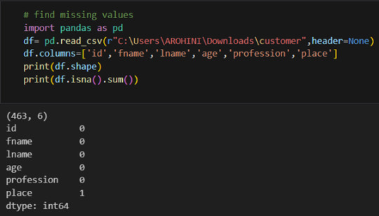
1. Identifying Missing Data Before handling missing values, it is important to detect them using functions like .isnull() in Python’s Pandas library. Understanding the pattern of missing data (random or systematic) helps in selecting the best strategy.

2. Removing Missing Data

If the missing values are minimal (e.g., less than 5% of the dataset), you can remove the affected rows using dropna().

If entire columns contain a significant amount of missing data, they may be dropped if they are not crucial for analysis.

3. Imputation Techniques

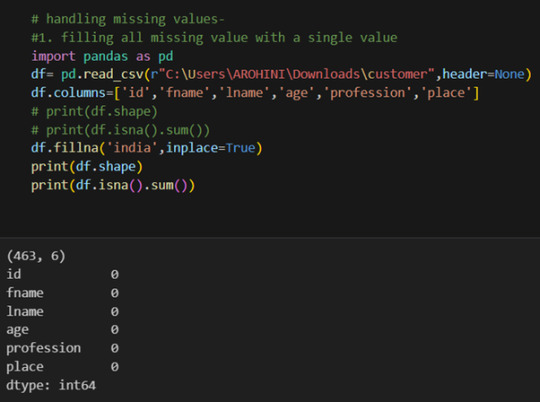
Mean/Median/Mode Imputation: For numerical data, replacing missing values with the mean, median, or mode of the column ensures continuity in the dataset.

Forward or Backward Fill: For time-series data, forward filling (ffill()) or backward filling (bfill()) propagates values from previous or next entries.

Interpolation: Using methods like linear or polynomial interpolation estimates missing values based on trends in the dataset.

Predictive Modeling: More advanced techniques use machine learning models like K-Nearest Neighbors (KNN) or regression to predict and fill missing values.

4. Using Algorithms That Handle Missing Data Some machine learning algorithms, like decision trees and random forests, can handle missing values internally without imputation.

By applying these techniques, data quality is improved, leading to more accurate insights. To master such data preprocessing techniques, consider enrolling in the best data analytics certification, which provides hands-on training in handling real-world datasets.

[learning-code-ficusoft]

Common techniques for feature selection and transformation

Feature selection and transformation are crucial steps in feature engineering to enhance machine learning model performance.

1️⃣ Feature Selection Techniques

Feature selection helps in choosing the most relevant features while eliminating redundant or irrelevant ones.

🔹 1. Filter Methods

These techniques evaluate features independently of the model using statistical tests. ✅ Methods:

Correlation Analysis → Select features with a high correlation with the target.

Chi-Square Test → Measures dependency between categorical features and the target variable.

Mutual Information (MI) → Evaluates how much information a feature provides about the target.

📌 Example (Correlation in Python)pythonimport pandas as pddf = pd.DataFrame({'Feature1': [1, 2, 3, 4, 5], 'Feature2': [10, 20, 30, 40, 50], 'Target': [0, 1, 0, 1, 0]}) correlation_matrix = df.corr() print(correlation_matrix)

🔹 2. Wrapper Methods

These methods use a machine learning model to evaluate feature subsets. ✅ Methods:

Recursive Feature Elimination (RFE) → Iteratively removes the least important features.

Forward/Backward Selection → Adds/removes features step by step based on model performance.

📌 Example (Using RFE in Python)pythonfrom sklearn.feature_selection import RFE from sklearn.ensemble import RandomForestClassifiermodel = RandomForestClassifier() selector = RFE(model, n_features_to_select=2) # Select top 2 features selector.fit(df[['Feature1', 'Feature2']], df['Target']) print(selector.support_) # True for selected features

🔹 3. Embedded Methods

These methods incorporate feature selection within model training. ✅ Examples:

Lasso Regression (L1 Regularization) → Shrinks coefficients of less important features to zero.

Decision Trees & Random Forest Feature Importance → Selects features based on their contribution to model performance.

📌 Example (Feature Importance in Random Forest)pythonmodel.fit(df[['Feature1', 'Feature2']], df['Target']) print(model.feature_importances_) # Higher values indicate more important features

2️⃣ Feature Transformation Techniques

Feature transformation modifies data to improve model accuracy and efficiency.

🔹 1. Normalization & Standardization

Ensures numerical features are on the same scale. ✅ Methods:

Min-Max Scaling → Scales values between 0 and 1.

Z-score Standardization → Centers data around mean (0) and standard deviation (1).

📌 Example (Scaling in Python)pythonfrom sklearn.preprocessing import MinMaxScaler, StandardScalerscaler = MinMaxScaler() df[['Feature1', 'Feature2']] = scaler.fit_transform(df[['Feature1', 'Feature2']])

🔹 2. Encoding Categorical Variables

Converts categorical data into numerical format for ML models. ✅ Methods:

One-Hot Encoding → Creates binary columns for each category.

Label Encoding → Assigns numerical values to categories.

📌 Example (One-Hot Encoding in Python)pythodf = pd.get_dummies(df, columns=['Category'])

🔹 3. Feature Extraction (Dimensionality Reduction)

Reduces the number of features while retaining important information. ✅ Methods:

Principal Component Analysis (PCA) → Converts features into uncorrelated components.

Autoencoders (Deep Learning) → Uses neural networks to learn compressed representations.

https://www.ficusoft.in/deep-learning-training-in-chennai/from sklearn.decomposition import PCApca = PCA(n_components=2) reduced_features = pca.fit_transform(df[['Feature1', 'Feature2']]

🔹 4. Log & Power Transformations

Used to make skewed data more normally distributed. ✅ Methods:

Log Transformation → Helps normalize right-skewed data.

Box-Cox Transformation → Used for normalizing data in regression models.

📌 Example (Log Transformation in Python)pythonimport numpy as npdf['Feature1'] = np.log(df['Feature1'] + 1) # Avoid log(0) by adding 1

Conclusion

✅ Feature Selection helps remove irrelevant or redundant features. ✅ Feature Transformation ensures better model performance by modifying features.

WEBSITE: https://www.ficusoft.in/deep-learning-training-in-chennai/

[masongrizchel]

Coding Diaries: Data Cleaning with Pandas (p2)

In my last post, I talked about how Pandas makes data cleaning more efficient. But as I dive deeper into real-world datasets, I’ve realized that data cleaning is rarely as simple as filling in missing values or removing duplicates. Unexpected challenges always pop up, forcing me to rethink my approach.

This post is about the messy, sometimes frustrating, but ultimately rewarding journey of cleaning real data—beyond just running a few Pandas functions.

When Standard Fixes Aren’t Enough

1. Dealing with Messy Text Data

One of the biggest surprises in data cleaning? Text columns that look fine—until you try to use them. Recently, I worked with a dataset where a "Category" column had inconsistent capitalization, extra spaces, and even hidden special characters.

Lesson learned: Never trust text data at first glance. Always check for inconsistencies.

2. The Hidden Danger of Missing Values

Missing values aren’t just blank cells. Sometimes, they show up as "NULL", "N/A", or even " - " in a dataset. Pandas treat these as text, not missing values.

This saved me hours of debugging later when I realized why my "empty" values weren’t actually being treated as NaNs.

Lesson learned: Always define missing values explicitly. Don’t assume Pandas will catch everything.

3. Unexpected Duplicates

Duplicate rows seem easy to fix, right? But what if some duplicates are partial? In a dataset of customer transactions, I found multiple entries with the same name but slightly different addresses. 

Pandas wouldn't treat these as duplicates, even though they refer to the same person. A quick fix was to standardize addresses before removing duplicates:

Lesson learned: Not all duplicates are identical. Standardizing data first makes a huge difference.

The Reality of Data Cleaning

Every dataset has its quirks. Some issues are easy to fix, while others require deeper investigation. What I’ve realized is that data cleaning isn’t just about applying Pandas functions—it’s about understanding the data, spotting inconsistencies, and making informed decisions about how to handle them.

Pandas is an incredible tool, but no function can replace a careful review of your dataset. Each cleaning step should be intentional, documented, and, when possible, automated for future use.

I’m still learning, but one thing’s for sure—cleaning data is just as important as analyzing it. Have you encountered any tricky data-cleaning challenges? Let’s discuss this in the comments!

[fromdevcom]

Pandas DataFrame Cleanup: Master the Art of Dropping Columns Data cleaning and preprocessing are crucial steps in any data analysis project. When working with pandas DataFrames in Python, you'll often encounter situations where you need to remove unnecessary columns to streamline your dataset. In this comprehensive guide, we'll explore various methods to drop columns in pandas, complete with practical examples and best practices. Understanding the Basics of Column Dropping Before diving into the methods, let's understand why we might need to drop columns: Remove irrelevant features that don't contribute to analysis Eliminate duplicate or redundant information Clean up data before model training Reduce memory usage for large datasets Method 1: Using drop() - The Most Common Approach The drop() method is the most straightforward way to remove columns from a DataFrame. Here's how to use it: pythonCopyimport pandas as pd # Create a sample DataFrame df = pd.DataFrame( 'name': ['John', 'Alice', 'Bob'], 'age': [25, 30, 35], 'city': ['New York', 'London', 'Paris'], 'temp_col': [1, 2, 3] ) # Drop a single column df = df.drop('temp_col', axis=1) # Drop multiple columns df = df.drop(['city', 'age'], axis=1) The axis=1 parameter indicates we're dropping columns (not rows). Remember that drop() returns a new DataFrame by default, so we need to reassign it or use inplace=True. Method 2: Using del Statement - The Quick Solution For quick, permanent column removal, you can use Python's del statement: pythonCopy# Delete a column using del del df['temp_col'] Note that this method modifies the DataFrame directly and cannot be undone. Use it with caution! Method 3: Drop Columns Using pop() - Remove and Return The pop() method removes a column and returns it, which can be useful when you want to store the removed column: pythonCopy# Remove and store a column removed_column = df.pop('temp_col') Advanced Column Dropping Techniques Dropping Multiple Columns with Pattern Matching Sometimes you need to drop columns based on patterns in their names: pythonCopy# Drop columns that start with 'temp_' df = df.drop(columns=df.filter(regex='^temp_').columns) # Drop columns that contain certain text df = df.drop(columns=df.filter(like='unused').columns) Conditional Column Dropping You might want to drop columns based on certain conditions: pythonCopy# Drop columns with more than 50% missing values threshold = len(df) * 0.5 df = df.dropna(axis=1, thresh=threshold) # Drop columns of specific data types df = df.select_dtypes(exclude=['object']) Best Practices for Dropping Columns Make a Copy First pythonCopydf_clean = df.copy() df_clean = df_clean.drop('column_name', axis=1) Use Column Lists for Multiple Drops pythonCopycolumns_to_drop = ['col1', 'col2', 'col3'] df = df.drop(columns=columns_to_drop) Error Handling pythonCopytry: df = df.drop('non_existent_column', axis=1) except KeyError: print("Column not found in DataFrame") Performance Considerations When working with large datasets, consider these performance tips: Use inplace=True to avoid creating copies: pythonCopydf.drop('column_name', axis=1, inplace=True) Drop multiple columns at once rather than one by one: pythonCopy# More efficient df.drop(['col1', 'col2', 'col3'], axis=1, inplace=True) # Less efficient df.drop('col1', axis=1, inplace=True) df.drop('col2', axis=1, inplace=True) df.drop('col3', axis=1, inplace=True) Common Pitfalls and Solutions Dropping Non-existent Columns pythonCopy# Use errors='ignore' to skip non-existent columns df = df.drop('missing_column', axis=1, errors='ignore') Chain Operations Safely pythonCopy# Use method chaining carefully df = (df.drop('col1', axis=1) .drop('col2', axis=1) .reset_index(drop=True)) Real-World Applications Let's look at a practical example of cleaning a dataset: pythonCopy# Load a messy dataset df = pd.read_csv('raw_data.csv')

# Clean up the DataFrame df_clean = (df.drop(columns=['unnamed_column', 'duplicate_info']) # Remove unnecessary columns .drop(columns=df.filter(regex='^temp_').columns) # Remove temporary columns .drop(columns=df.columns[df.isna().sum() > len(df)*0.5]) # Remove columns with >50% missing values ) Integration with Data Science Workflows When preparing data for machine learning: pythonCopy# Drop target variable from features X = df.drop('target_variable', axis=1) y = df['target_variable'] # Drop non-numeric columns for certain algorithms X = X.select_dtypes(include=['float64', 'int64']) Conclusion Mastering column dropping in pandas is essential for effective data preprocessing. Whether you're using the simple drop() method or implementing more complex pattern-based dropping, understanding these techniques will make your data cleaning process more efficient and reliable. Remember to always consider your specific use case when choosing a method, and don't forget to make backups of important data before making permanent changes to your DataFrame. Now you're equipped with all the knowledge needed to effectively manage columns in your pandas DataFrames. Happy data cleaning!

[ensafomer]

"Using K-Means Clustering to Identify Data Groups: Applications and Clustering Techniques

To perform k-means clustering on your dataset, follow these steps using Python and libraries like pandas, scikit-learn, and matplotlib. Below are the steps you need to follow to complete the task.

1. Load and Clean the Data:

First, you need to load your dataset using pandas. Ensure the data is ready for analysis (remove missing values or handle unnecessary columns).

2. Import Required Libraries

3. Load the Dataset:

As

sume your dataset is stored in a CSV file:

4. Select Variables for Clustering:

Make sure to choose the quantitative variables you will use for k-means analysis. If you have categorical variables, you may need to convert them into numeric variables using encoding techniques like One-Hot Encoding.

5. Choose the Number of Clusters k:

Choosing the right number of clusters is crucial. You can use the Elbow Method to find the ideal number of clusters:

Based on the graph, choose the value of k where the elbow (or "bend") occurs.

6. Run the k-means Clustering:

7. Add Clusters to the Dataset:

8. Display the Results:

Now you can view the data with the clusters added and see how the observations have been grouped:

9. Plot the Clusters:

To visualize the clusters, you can use matplotlib:

10. Summarize the Results:

Formula Used: Include the code used to perform the clustering.

Outputs: Provide the output related to the clusters identified.

Summary: Explain how the analysis showed that the data can be divided into certain groups based on the studied variables.

Outputs: The data was divided into 3 clusters as follows:

Cluster 1: Contains observations with characteristics A and B.

Cluster 2: Contains observations with characteristics C and D.

Cluster 3: Contains observations with characteristics E and F.

Summary: Using k-means clustering, the data was divided into three main clusters. This analysis helps identify patterns within the data, such as grouping observations with similar responses on the selected variables.

[asquaretechnologies]

Beginner’s Guide: Data Analysis with Pandas

Data analysis is the process of sorting through all the data, looking for patterns, connections, and interesting things. It helps us make sense of information and use it to make decisions or find solutions to problems. When it comes to data analysis and manipulation in Python, the Pandas library reigns supreme. Pandas provide powerful tools for working with structured data, making it an indispensable asset for both beginners and experienced data scientists.

What is Pandas?

Pandas is an open-source Python library for data manipulation and analysis. It is built on top of NumPy, another popular numerical computing library, and offers additional features specifically tailored for data manipulation and analysis. There are two primary data structures in Pandas:

• Series: A one-dimensional array capable of holding any type of data.

• DataFrame: A two-dimensional labeled data structure similar to a table in relational databases.

It allows us to efficiently process and analyze data, whether it comes from any file types like CSV files, Excel spreadsheets, SQL databases, etc.

How to install Pandas?

We can install Pandas using the pip command. We can run the following codes in the terminal.

After installing, we can import it using:

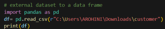
How to load an external dataset using Pandas?

Pandas provide various functions for loading data into a data frame. One of the most commonly used functions is pd.read_csv() for reading CSV files. For example:

The output of the above code is:

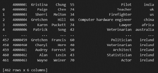
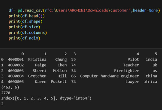
Once your data is loaded into a data frame, you can start exploring it. Pandas offers numerous methods and attributes for getting insights into your data. Here are a few examples:

df.head(): View the first few rows of the DataFrame.

df.tail(): View the last few rows of the DataFrame.

http://df.info(): Get a concise summary of the DataFrame, including data types and missing values.

df.describe(): Generate descriptive statistics for numerical columns.

df.shape: Get the dimensions of the DataFrame (rows, columns).

df.columns: Access the column labels of the DataFrame.

df.dtypes: Get the data types of each column.

In data analysis, it is essential to do data cleaning. Pandas provide powerful tools for handling missing data, removing duplicates, and transforming data. Some common data-cleaning tasks include:

Handling missing values using methods like df.dropna() or df.fillna().

Removing duplicate rows with df.drop_duplicates().

Data type conversion using df.astype().

Renaming columns with df.rename().

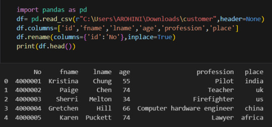
Pandas excels in data manipulation tasks such as selecting subsets of data, filtering rows, and creating new columns. Here are a few examples:

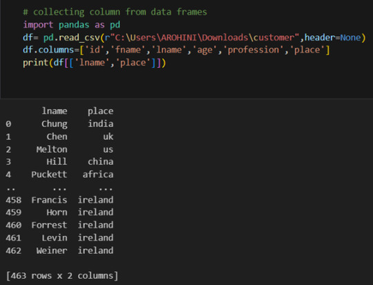
Selecting columns: df[‘column_name’] or df[[‘column1’, ‘column2’]].

Filtering rows based on conditions: df[df[‘column’] > value].

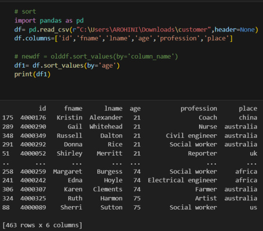
Sorting data: df.sort_values(by=’column’).

Grouping data: df.groupby(‘column’).mean().

With data cleaned and prepared, you can use Pandas to perform various analyses. Whether you’re computing statistics, performing exploratory data analysis, or building predictive models, Pandas provides the tools you need. Additionally, Pandas integrates seamlessly with other libraries such as Matplotlib and Seaborn for data visualization

[anushakowkuntla]

Coursera-Data Management and Visualization-week 2- Assignment

1) Your program: --------------My Code---------

#import libraries

import pandas as pd import numpy as np

#bug fix to avoid run time errors

pd.set_option('display.float_format', lambda x:'%f'%x)

#read the dataset

data = pd.read_csv(r"C:/Users/AL58114/Downloads/gapminder.csv")

#print the total number of observations in the dataset.

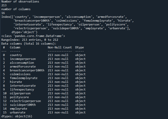
print("Number of observations") print(len(data))

#print number of columns count

print("number of columns") print(len(data.columns))

#print to see the column names

print(data.columns)

print(data.info())

data_cleaned = pd.DataFrame(data , columns = ['country','employrate','urbanrate','oilperperson'])

data_cleaned = data_cleaned.replace(r'\s+', np.nan, regex = True) data_cleaned['employrate']=data_cleaned['employrate'].astype('float64') data_cleaned['urbanrate']=data_cleaned['urbanrate'].astype('float64') data_cleaned['oilperperson']=data_cleaned['oilperperson'].astype('float64')

print(data_cleaned.info())

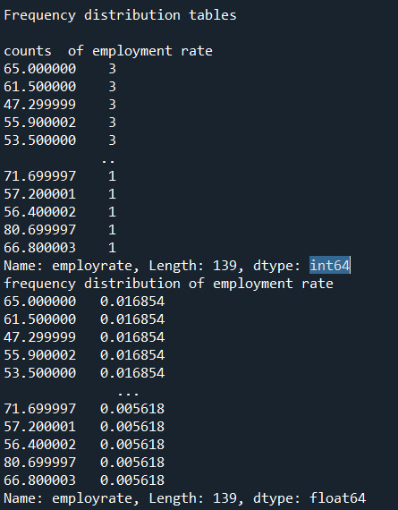
print("\nFrequency distribution tables\n") print("counts of employment rate") print(data_cleaned['employrate'].value_counts())

print("frequency distribution of employment rate") print(data_cleaned['employrate'].value_counts(normalize = True))

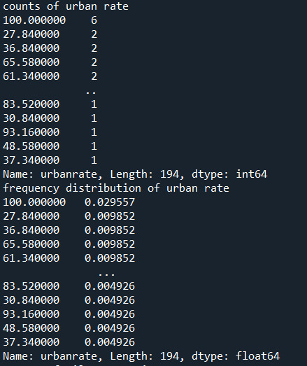
print("counts of urban rate") print(data_cleaned['urbanrate'].value_counts())

print("frequency distribution of urban rate") print(data_cleaned['urbanrate'].value_counts(normalize = True))

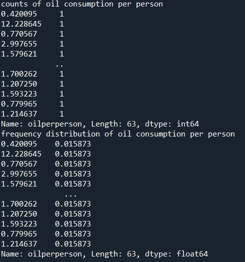
print("counts of oil consumption per person") print(data_cleaned['oilperperson'].value_counts())

print("frequency distribution of oil consumption per person") print(data_cleaned['oilperperson'].value_counts(normalize = True))

---------------End of code----------

2) the output that displays three of your variables as frequency tables

Below are the outputs displayed for each variable on the anaconda console window. Since the output is too long for reasons I have pasted them in parts.

3) a few sentences describing your frequency distributions in terms of the values the variables take, how often they take them, the presence of missing data, etc.

Summary:

I added additional Pandas functions to help visualize the data below.

There was no need to subset the data since it's already aggregated per country. The 3 chosen variables span 213 countries and I would like to include each country in my study.

Typically, I would drop the blank cells from my percent calculations below, however the Python code we were presented with this week had "dropna=false".

Each of the 3 chosen GapMinder columns\variables has missing data. Removing the missing data from each column may not affect the overall research questions, however the same rows have different missing data, thus in aggregate removing all rows with missing values will likely have an impact on the research questions.

Rather than remove the rows with missing data another approach is to calculate the column mean and add it to the missing cells.

Variable Details:

Employ Rate:

"Employment rate" shows the number of times a particular Employment rate occurred. For example, a employe rate of 52.8 occurred 2 times in the data set.  

"Employe rate" is the number of times a particular employe rate occurred divided by the count of all employe rates, There are 213 countries\rows which also include blank cells.

Urban Rate:

Urban rate shows the rate of people living in urban areas. There are missing data in some countries. There are 2 countries with the maximum rate of 100 in the dataset.

"Urban Rate" is the number of times at which population of urban areas occurred divided by the count of all the urban rates. There are 213 countries in the whole dataset.

Oil per person:

"oilperperson" refers to the oil consumption per person on yearly basis. There are a lot of blank cells in the gapminder dataset. 70% percent of the countries oil per person consumption lies between 0-2. In the countries with high urban rate their seems to be more oil consumption per person.

[subashdhoni86]

Dummy Variables & One Hot Encoding

Handling Categorical Variables with One-Hot Encoding in Python

Introduction:

Machine learning models are powerful tools for predicting outcomes based on numerical data. However, real-world datasets often include categorical variables, such as city names, colors, or types of products. Dealing with categorical data in machine learning requires converting them into numerical representations. One common technique to achieve this is one-hot encoding. In this tutorial, we will explore how to use pandas and scikit-learn libraries in Python to perform one-hot encoding and avoid the dummy variable trap.

1. Understanding Categorical Variables and One-Hot Encoding:

Categorical variables are those that represent categories or groups, but they lack a numerical ordering or scale. Simple label encoding assigns numeric values to categories, but this can lead to incorrect model interpretations. One-hot encoding, on the other hand, creates binary columns for each category, representing their presence or absence in the original data.

2. Using pandas for One-Hot Encoding:

To demonstrate the process, let's consider a dataset containing information about home prices in different towns.

import pandas as pd

# Assuming you have already loaded the data

df = pd.read_csv("homeprices.csv")

print(df.head())

The dataset looks like this:

       town area  price

0 monroe township 2600 550000

1 monroe township 3000 565000

2 monroe township 3200 610000

3 monroe township 3600 680000

4 monroe township 4000 725000

Now, we will use `pd.get_dummies` to perform one-hot encoding for the 'town' column:

dummies = pd.get_dummies(df['town'])

merged = pd.concat([df, dummies], axis='columns')

final = merged.drop(['town', 'west windsor'], axis='columns')

print(final.head())

The resulting DataFrame will be:

  area  price monroe township robinsville

0 2600 550000        1      0

1 3000 565000        1      0

2 3200 610000        1      0

3 3600 680000        1      0

4 4000 725000        1      0

3. Dealing with the Dummy Variable Trap:

The dummy variable trap occurs when there is perfect multicollinearity among the encoded variables. To avoid this, we drop one of the encoded columns. However, scikit-learn's `OneHotEncoder` automatically handles the dummy variable trap. Still, it's good practice to handle it manually.

# Manually handle dummy variable trap

final = final.drop(['west windsor'], axis='columns')

print(final.head())

The updated DataFrame after dropping the 'west windsor' column will be:

  area  price monroe township robinsville

0 2600 550000        1      0

1 3000 565000        1      0

2 3200 610000        1      0

3 3600 680000        1      0

4 4000 725000        1      0

4. Using sklearn's OneHotEncoder:

Alternatively, we can use scikit-learn's `OneHotEncoder` to handle one-hot encoding:

from sklearn.preprocessing import OneHotEncoder

from sklearn.compose import ColumnTransformer

# Assuming 'df' is loaded with town names already label encoded

X = df[['town', 'area']].values

y = df['price'].values

# Specify the column(s) to one-hot encode

ct = ColumnTransformer([('town', OneHotEncoder(), [0])], remainder='passthrough')

X = ct.fit_transform(X)

# Remove one of the encoded columns to avoid the trap

X = X[:, 1:]

5. Building a Linear Regression Model:

Finally, we build a linear regression model using the one-hot encoded data:

from sklearn.linear_model import LinearRegression

model = LinearRegression()

model.fit(X, y)

# Predicting home prices for new samples

sample_1 = [[0, 1, 3400]] 

sample_2 = [[1, 0, 2800]] 

Conclusion:

One-hot encoding is a valuable technique to handle categorical variables in machine learning models. It converts categorical data into a numerical format, enabling the use of these variables in various algorithms. By understanding the dummy variable trap and appropriately encoding the data, we can build accurate predictive models. In this tutorial, we explored how to perform one-hot encoding using both pandas and scikit-learn libraries, providing clear examples and code snippets for easy implementation.

@talentserve

[analysisbyzee]

Classification Decision Tree for Heart Attack Analysis

Primarily, the required dataset is loaded. Here, I have uploaded the dataset available at Kaggle.com in the csv format.

All python libraries need to be loaded that are required in creation for a classification decision tree. Following are the libraries that are necessary to import:

The following code is used to load the dataset. read_csv() function is used to load the dataset.

column_names = ['age','sex','chest pain','resting blood pressure','cholestrol','fasting blood sugar','resting ecg','max heart rate','excercise included','old peak','slp','caa','THALL','output']

data= pd.read_csv("heart.csv",header=None,names=column_names)

data = data.iloc[1: , :] # removes the first row of dataframe

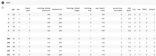
Now, we divide the columns in the dataset as dependent or independent variables. The output variable is selected as target variable for heart disease prediction system. The dataset contains 13 feature variables and 1 target variable.

feature_cols = ['age','sex','chest pain','chest pain','resting blood pressure','cholestrol','fasting blood sugar','resting ecg','max heart rate','excercise included','old peak','slp','caa','THALL']

pred = data[feature_cols] # Features

tar = data.output # Target variable

Now, dataset is divided into a training set and a test set. This can be achieved by using train_test_split() function. The size ratio is set as 60% for the training sample and 40% for the test sample.

pred_train, pred_test, tar_train, tar_test = train_test_split(X, y, test_size=0.4, random_state=1)

Using the shape function, we observe that the training sample has 181 observations (nearly 60% of the original sample) and 10 explanatory variables whereas the test sample contains 122 observations(nearly 40 % of the original sample) and 10 explanatory variables.

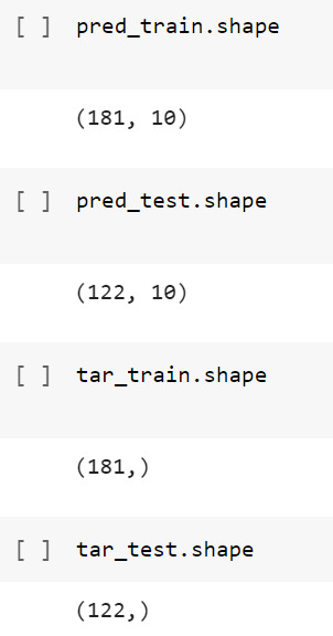
Now, we need to create an object claf_mod to initialize the decision tree classifer. The model is then trained using the fit function which takes training features and training target variables as arguments.

# To create an object of Decision Tree classifer

claf_mod = DecisionTreeClassifier()

# Train the model

claf_mod = claf_mod.fit(pred_train,tar_train)

To check the accuracy of the model, we use the accuracy_score function of metrics library. Our model has a classification rate of 58.19 %. Therefore, we can say that our model has good accuracy for finding out a person has a heart attack.

To find out the correct and incorrect classification of decision tree, we use the confusion matrix function. Our model predicted 18 true negatives for having a heart disease and 53 true positives for having a heart attack. The model also predicted 31 false negatives and 20 false positives for having a heart attack.

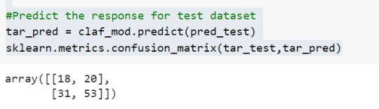
To display the decision tree we use export_graphviz function. The resultant graph is unpruned.

dot_data = StringIO()

export_graphviz(claf_mod, out_file=dot_data,

filled=True, rounded=True,

special_characters=True,class_names=['0','1'])

graph = pydotplus.graph_from_dot_data(dot_data.getvalue())

graph.write_png('heart attack.png')

Image(graph.create_png())

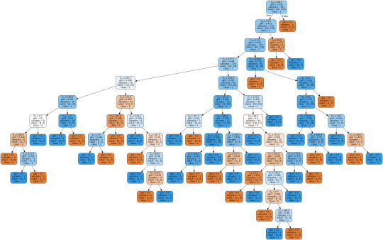
To get a prune graph, we changed the criterion as entropy and initialized the object again. The maximum depth of the tree is set as 3 to avoid overfitting.

# Create Decision Tree classifer object

claf_mod = DecisionTreeClassifier(criterion="entropy", max_depth=3)

# Train Decision Tree Classifer

claf_mod = claf_mod.fit(pred_train,tar_train)

#Predict the response for test dataset

tar_pred = claf_mod.predict(pred_test)

By optimizing the performance, the classification rate of the model increased to 72.13%.

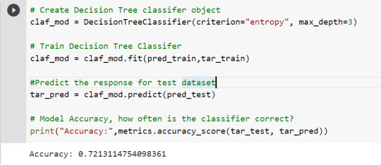
By passing the object again into export_graphviz function, we obtain the prune graph.

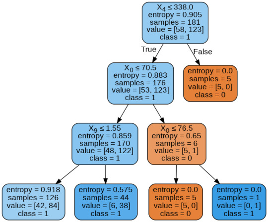
From the above graph, we can infer that :

1) individuals having cholesterol less than 338 mg/dl, age less than or equal to 70.5 years, and whose previous peak was less than or equal to 1.55: 84 of them are more likely to have a heart attack whereas 42 of them will less likely to have a heart attack.

2) individuals having cholesterol less than 338 mg/dl, age less than or equal to 70.5 years, and whose previous peak was more than 1.55: 6 of them will less likely to have a heart attack whereas 38 of them are more likely to have a heart attack.

3) individuals having cholesterol less than 338 mg/dl and age less than or equal to 76.5 years: are less likely to have a heart attack

4) individuals having cholesterol less than 338 mg/dl and age more than 76.5 years: are more likely to have a heart attack

5) individuals having cholesterol more than 338 mg/dl : are less likely to have a heart attack

The Whole Code:

from google.colab import files uploaded = files.upload()

import pandas as pd from sklearn.tree import DecisionTreeClassifier # Import Decision Tree Classifier from sklearn.model_selection import train_test_split # Import train_test_split function from sklearn.metrics import classification_report import sklearn.metrics #Import scikit-learn metrics module for accuracy calculation from sklearn.tree import export_graphviz from sklearn.externals.six import StringIO from IPython.display import Image import pydotplus

column_names = ['age','sex','chest pain','resting blood pressure','cholestrol','fasting blood sugar','resting ecg','max heart rate','excercise included','old peak','slp','caa','THALL','output'] data= pd.read_csv("heart.csv",header=None,names=column_names) data = data.iloc[1: , :] # removes the first row of dataframe (In this case, ) #split dataset in features and target variable feature_cols = ['age','sex','chest pain','chest pain','resting blood pressure','cholestrol','fasting blood sugar','resting ecg','max heart rate','excercise included','old peak','slp','caa','THALL'] pred = data[feature_cols] # Features tar = data.output # Target variable pred_train, pred_test, tar_train, tar_test = train_test_split(X, y, test_size=0.4, random_state=1) # 60% training and 40% test pred_train.shape pred_test.shape tar_train.shape tar_test.shape

# To create an object of Decision Tree classifer claf_mod = DecisionTreeClassifier() # Train the model claf_mod = claf_mod.fit(pred_train,tar_train) #Predict the response for test dataset tar_pred = claf_mod.predict(pred_test) sklearn.metrics.confusion_matrix(tar_test,tar_pred) # Model Accuracy, how often is the classifier correct? print("Accuracy:",metrics.accuracy_score(tar_test, tar_pred)) dot_data = StringIO() export_graphviz(claf_mod, out_file=dot_data, filled=True, rounded=True, special_characters=True,class_names=['0','1']) graph = pydotplus.graph_from_dot_data(dot_data.getvalue()) graph.write_png('heart attack.png') Image(graph.create_png())

# Create Decision Tree classifer object claf_mod = DecisionTreeClassifier(criterion="entropy", max_depth=3) # Train Decision Tree Classifer claf_mod = claf_mod.fit(pred_train,tar_train) #Predict the response for test dataset tar_pred = claf_mod.predict(pred_test) # Model Accuracy, how often is the classifier correct? print("Accuracy:",metrics.accuracy_score(tar_test, tar_pred)) from sklearn.externals.six import StringIO from IPython.display import Image from sklearn.tree import export_graphviz import pydotplus dot_data = StringIO() export_graphviz(claf_mod, out_file=dot_data, filled=True, rounded=True, special_characters=True, class_names=['0','1']) graph = pydotplus.graph_from_dot_data(dot_data.getvalue()) graph.write_png('improved heart attack.png') Image(graph.create_png())

[alj4890]

A Second Chance

(Thomas Hunt x oc*Amanda)

A/N Our last chapter of this series. I will say that some things did not turn out how I originally planned, but I do love that about writing with these characters. They really do end up taking a life of their own. Our final chapter for A Second Chance has Maxwell’s big surprise, Amanda’s decision, and an epilogue. Thanks so much for enjoying this brief series. Sorry I haven’t responded much on your comments. In between beginning this and ending it, migraines from the bowels of the earth struck at various intervals. But I have thoroughly enjoyed how this story unfolded.

@lxaah11 @alleksa16 @penguininapinktuxedo​ @blackcoffee85 @stopforamoment  @hopefulmoonobject   @krsnlove   @annekebbphotography @hopelessromantic1352 . @sunflowergirl05  @desireepow-1986 @greywitchyshots @lilyofchoices @moodyvalentinestories @emceesynonymroll @my-heart-beats-for-ya @aworldoffandoms @ab1901  @flyawayboo @i-bloody-love-drake-walker . @trappedinfandoms  @kate-mckenzie @cordoniaqueensworld @everythingmarvelsherlockspn

Masterlist

Catch up here with Chapter 9

Chapter 10

While Maxwell was away, Amanda sat down and begin to compose a list of all the things at St Orella that were either left to her as an inheritance or she had purchased herself. Everything else either was left in terms of being a part of the duchy.

Thomas had read Kathleen a few stories at the window seat while she continued to write down what she knew was hers. He would look up every once in a while and watch her tap the top of her pen to her lips while reading over what she had listed.

When she set it down, he realized that her list barely covered half a page.

As Kathleen left them to see what her aunt and uncle were doing, Thomas came up behind Amanda’s chair and read over her shoulder. “That’s all you plan to take?”

She nodded. “The majority of furniture was left to the St Orellan heir. These are what members of my family either left personally to me or to a family member who then made certain I inherited it.” She then pointed to another column. “These I bought for myself using my personal fortune and not the St. Orellan coffers.”

“What about the portraits of your parents and uncle?” He asked.

She shook her head. “Those were painted for the St Orellan gallery.” When she noticed his concern, she gently caressed his cheek. “I have plenty of pictures of them that will go with me.” She then opened a drawer to her desk. “And I get to take these with me.” She pulled out the different journals of her ancestors. “Each one was written for family, not the for the current duke or duchess.”

He pressed a kiss to her lips when she looked back up at him.

“You know Maxwell won’t mind if you take more.” He kissed her ear. “I don’t want you to leave behind anything that means something to you.”

She smiled and shook her head. “I am taking what means the most to me.” She looked up at all the heavily ornate furniture and decorations, excited at the prospect of picking new décor. “The rest belongs here.”

He took her hand when she rose from her chair. She met his still worried gaze and smiled. “Come. Let’s get Kathleen ready for this big surprise.”

*************

A little over an hour later…

"Must we wear these?" Thomas asked.

Maxwell nodded. "It's the only way for you to be truly surprised."

Kathleen obediently slipped on the sleep mask and gripped her mother's shirt.

"Wait until we are in the car." Amanda said, trying to keep from laughing.

"It isn't a surprise party, is it?" Thomas appeared suddenly ill.

"You'll find out soon enough." Maxwell said in a sing song voice.

Kathleen giggled at her father's resigned expression. He glanced down at her, saw she only had one eye covered with the sleep mask, and felt his first smile form since Maxwell had handed them the blinders.

"What do you think the surprise is?" He whispered to her.

"Maybe a party." Kathleen said. "Oh! Or an animal!" Her face lit up with excitement. "He gave Aunt Riley and Uncle Liam two red pandas when they got married. What if he got us two since you and Mommy are getting married."

Maxwell heard her loud whisper and gently shook his head no when Amanda whispered to him if it was that.

"I never do repeats." He admitted. "I'm not that kind of gifter."

"A limo?" Thomas' eyebrows raised in disbelief when they followed him outside. "Where are we going?"

"You can't expect my surprise to begin with a normal car ride." Maxwell replied, wounded at such a thought.

Kathleen hurried inside.

"After you." Maxwell said to the couple.

The two got in and sat down across from their daughter. Maxwell smoothly slid in and sat on the seat between Kathleen and her parents.

He rubbed his hands together. "Alright party people, masks on!"

Thomas groaned softly when both Amanda and Kathleen gave him a silent pleading look to play along. He pulled the mask over his head and settled it over his eyes. He felt somewhat placated for doing so when he felt a kiss placed on his cheek

Once everyone had their sleep masks firmly in place, Maxwell lowered the privacy barrier and told the driver to proceed. He raised it back up and relaxed with a big smile on his face.

During the long ride, Thomas felt Amanda slip her hand in his as well as resting her head against his shoulder. His lips curved as memories of the night before flashed through his mind. He was looking forward to tonight and all the possibilities that were before him.

Amanda’s own smile appeared when she felt his arm lift to wrap around her. She then felt his lips brush her temple and couldn't wait until they were alone once more. Her heart was completely ready for their future. Now that the burden of St Orella had been lifted off of her shoulders, she was excited for what lay ahead.

The two had stayed up late into the night making plans for the type of wedding they wanted, possible honeymoon destinations, and of course talk of maybe having more children.

Even when she used to daydream of Thomas realizing he loved her and wanted to be with her and Kathleen, it had never matched to the real thing. She still was waiting on either her alarm clock or Kathleen to wake her up from what surely must be a dream.

While the two sat quietly with their thoughts, Kathleen kept up a steady chatter with Maxwell, trying to guess where they were going.

"Give it up, Kat." Maxwell teased. "You will never guess this."

He had to fight his laughter at her huffing and folding her arms. Her little face scrunched into a fierce frown was made even more humorous by the sleep mask covering half of it.

After some time, the limo slowed to a stop.

"Keep those on!" Maxwell ordered when they all moved to rip the blinders off.

He got out, commanded they remained still, and then told them to carefully step out.

"Alright, stand right here--wait no--Thomas, you need to--" Maxwell repositioned them and stood in front of them to make certain they were in the best spot for the big reveal.

"It sounds like the beach." Kathleen gripped her parents' hands as she strained to figure out what their surprise was.

"Yes, it does." Thomas murmured.

"Is it a picnic?!" Kathleen asked.

Maxwell shook his head then realized none of them could see him. "No picnic."

"Are we going sailing?" Amanda asked.

"Nope." Maxwell gloated. "Now, on the count of three, I want you to take your masks off." He glanced behind him, grinning at his conspirators stepping out onto the lawn. "One...two...THREE!"

The family removed them and blinked at the bright sky.

They looked around curiously.

"Well?! What do you think?" Maxwell could not quite contain his giddy excitement.

"The house?" Thomas asked, looking at the mansion set against the rocky shore.

"It's beautiful." Amanda said, admiring the subdued gray brick.

"It's yours." Maxwell said proudly.

The couple looked at him with mouths agape.

"What?" Thomas uttered.

"Can we go in?" Kathleen asked.

"Maxwell--how, you can't give us a house!" Amanda exclaimed. "This is too much."

The rest of the Cordonian group and Stephen and Rachel had smiles as they pointed out that it was a wedding present from them all.

"Max picked it out." Riley began. "He said you had to have a place in Cordonia so that you would visit more often."

"Liam used his kingly authority and got all the paperwork completed overnight." Drake added.

"And we have been doing a little bit of decorating." Olivia rolled her eyes. "Mostly, we have been doing whatever Hana ordered us to do."

Amanda covered her mouth as tears filled her eyes. She shook her head at the immense generosity of her friends. They had stuck by her through every trial she faced. Helped her wade through years of uncertainty. And now they had rushed to give her a home all her own. No nobles to deal with. No political work to keep it. Just a home for her and her family.

When the first broken sob escaped her lips, Thomas gently pulled her into his arms. She tried to muffle her crying against his shirt.

"Mommy!" Kathleen rubbed her eyes and pressed her face against her legs. "Don't cry."

Thomas rubbed Amanda’s back while she tried to calm down. He knew the last few days had to be a whirlwind of change and stress on her. Being given such a gift was her breaking point.

Hudson cleared his throat from the front door. "Your grace?" When numerous heads turned toward him, he shook his head. "Forgive me, I meant Lady Hana. There is an issue of furniture placement that we need your direction on."

Hana smiled and hurried inside, pulling Rashad along with her.

"Hey," Maxwell said softly. He tugged on Amanda's hair making a surprise laugh pop out amongst her tears. "Can I give you your tour before I go pick up Nadia from the airport?"

She nodded while dabbing at her cheeks and nose with the tissues Riley had handed her.

He grinned and motioned with his head. "Come on. I can't wait for you to see the inside. It literally screams Amanda and Thomas."

Kathleen tugged on his hand. "What about me?"

His grin grew bigger. "Just you wait, Kat. Hana has done something that definitely has your name written all over it."

The rooms were bright and cheerful with unparalleled views of the ocean. They were also surprisingly filled with furniture.

Amanda paused when she recognized her favorite recliner from one of her informal dens at St Orella. "Max? Is this..."

"Don't worry." He said proudly. "Hudson knows what has to stay at St Orella and what doesn't. The rest though is new furniture." He shook his head as if to admonish her. "Every bride needs something old and something new."

Thomas laced his fingers with hers as they continued with the tour.

There were rooms for all their needs. A breakfast nook in the large kitchen. A dining room with Amanda's great grandmother's china tea set sitting in a place of honor in the middle of a table that could seat twelve. A study was currently being worked on by a few of St Orella's servants. Some of the books on the shelves were the very ones Kathleen had been interested in.

A large living room was complete with nothing but furniture that was made for comfort. No rough, formal antiques that made one less likely to sit could be found anywhere.

There was one room downstairs that was left completely empty.

"This will be the theater room." Maxwell explained. "I called Addison to let her know what we were doing, and she and the Hollywood bunch are designing this for you. They'll be here Monday."

Thomas groaned at the thought of more company. His lips curved though each time Amanda exclaimed how much she loved all that they had seen.

Kathleen tugged on Maxwell's hand. "Can we see my bedroom?"

"Bedroom?" He pretended to ponder that. "Hmm...did you need one?"

Her little jaw dropped. "Where will I sleep?"

"I didn't think of that." Maxwell muttered. He chuckled when she still seemed unable to believe it. "Do you honestly think I would leave out the most important part?"

They went up the staircase and saw a room with the door closed and another larger one with Hana directing some workers.

"Let's look at where we are going to stick your parents first." Maxwell whispered.

They all peeked into the room where Hana was.

"Oh!" Amanda gasped. The room was similar in design to the one she had in St Orella. There was a large fireplace in which Hana had placed two chairs. The bed that was being put together was set in a way that one could enjoy the fire from it or turn on their side and see the ocean.

Thomas admired the suite's bathroom with its large shower with multiple shower heads. His eyebrows lifted at some of their clothes already in the walk-in closet.

"Hana," Maxwell called out. "It is time to reveal your masterpiece!"

She smiled and left Rashad in charge.

"Close your eyes." Hana whispered as she held Kathleen's hand.

The little girl closed them tight and nearly bounced with anticipation when she heard the door open.

"You can open them." Hana clasped her hands together, beaming at the happiness she saw in Kathleen's face.

"Twinkle lights!" Kathleen pointed up at the ceiling. She went from one area to another, thanking Hana with each aspect she loved.

"Hana," Amanda said in surprise. "This looks so much like her room in California."

"I wanted her to have that sense of home here." Hana explained, blushing at all the compliments everyone was giving her. "That was why I asked you for more detail about her room." She knelt when Kathleen hugged her.

"This is the best surprise ever!” Kathleen told her, kissing her cheek. "I love my room, Aunt Hana."

Maxwell grinned and quietly motioned for Amanda to follow him. "The rest are guestrooms that we ran out of time to furnish. We thought you and Thomas and Kathleen might want to stay here tonight. Rachel and Stephen can stay at St Orella for as long as they want."

He rocked back and forth on the balls of his feet. "Are you happy with it?"

She nodded, pulling him into a hug. "More than I can express." She kissed his cheek and tried not to cry again. "Thank you."

He checked the time and told her he would be back later. "Hudson and the rest will be bringing your things over. Anything you want from St Orella is yours. Just write out a list and he'll make sure to have it delivered." He winked before hurrying down the stairs.

***************

While Kathleen played in her new room, Thomas and Amanda stepped outside to the back patio. It curved around with the house and had a number of lounge chairs and covered swings set out.

"What do you think?" Amanda asked.

"It's a beautiful home." He turned to look up at it. "I'm surprised Maxwell chose one that I would have actually picked for us."

He noticed she was staring at him. "What are you thinking?"

"That I want to get married." She admitted, blooms of color appearing on her cheeks.

He smiled as his lips tenderly brushed hers. "So do I."

"I mean today." She looked up at him. "I want our first night here to be one of us celebrating our marriage."

His arms tightened around her. "I will marry you whenever you wish." His lips grazed her ear. "Nothing could make me happier than doing so right now."

Amanda smiled as she met his lips in a more heated kiss. "Wait here."

He watched her hurry inside, disappearing down a hall.

A few minutes later she returned with Liam.

"You do realize that everyone will have my head for this?" He teased.

"We will do our best to be discreet." Amanda glanced at Thomas. "Or as discreet as we can be with dressing up."

"You have a plan?" Thomas asked, noticing the secretive smile on her face.

"I do." She pointed to a secluded area on the shore. "Meet us down there in thirty minutes."

*************

40 minutes later...

 Thomas tugged at his bowtie and checked the time once more.

"You're not nervous, are you?" Liam asked, amused watching his agitated movements.

"No." His frown eased. "Not at all. I'm about to marry the only one I have ever loved."

Liam clapped his shoulder in camaraderie.

"Can you legally marry us without witnesses?" Thomas asked, concerned about it not being official.

Liam nodded. "I'm the king. It will be legal and binding." His eyes lifted when he saw movement coming down the hill. "Ah, here they are."

Thomas turned and couldn't stop the smile that formed. Kathleen had on the sparkly dress he had bought her for her birthday. Amanda had dressed in the dark teal gown she had known he had always loved her in.

The two loves of his life walked hand in hand and stopped before him.

"We're ready." Kathleen said to Liam.

He chuckled and began the ceremony.

While Amanda and Thomas stood before one other with their hands clasped, Kathleen stood next to Liam. She leaned against his side as the vows were exchanged. He placed his hand on her shoulder and gently squeezed when she let out a yawn.

Her parents though were oblivious to her thinking it was taking too long. When Liam brought up the issue of rings, Amanda began to say they did not have any yet.

Thomas pulled them out of his pocket.

"Where did you get those?" She asked, completely surprised.

"I wanted them to match your engagement ring." Thomas lowered his eyes to the bands he held. "I bought them at the same time."

She shook her head while trying not to cry again. When she took his wedding ring, she noticed markings on the inside.

She held it closer and read the words aloud. "A second chance."

 He nodded at the engraving he had secretly had done while she was in the capital. Thomas slipped her ring over her finger and raised her hand to his lips, pressing a tender kiss to it. He lifted his eyes to hers. "That's been my wish for five years."

She slid his ring over his finger and pulled him close for a kiss. All the love they felt was poured into that single touch. She opened her eyes, smiling that this wasn't a dream. "It's been my wish too."

************

Epilogue…

Once upon a time, there was a duchess from a far away land who met a man from Hollywood. The instant they met; they knew that something special was about to happen. Over time they realized that they were in love. But like all fairy tales, turmoil struck and the two were forced to be apart for a long time. The only consolation the duchess had was in the little piece of her former relationship: a daughter.

The poor man in Hollywood, pining for his lost love, was left in the dark to her existence. Years of searching for the one who held his heart would all come to an end one fateful night in New York.

That was the moment for a second chance at love to occur. Fears and doubts plagued the couple, and yet they persevered in the hopes to one day be together. More trials and decisions were made until the moment they said I do on a rocky shore in Cordonia.

What was to follow surprised no one who knew the couple. The two settled into a happy life together. Thomas, our hero, continued to make movies and to love his wife and daughter with all his heart. He never took one moment he had with them for granted, having seen what life was like without them. He spent every moment he had making certain that they knew they were his entire world. Nothing else matter but his love and his family.

Amanda, our heroine, settled into a life as a stay-at-home mom. She and their daughter Kathleen supported and loved Thomas in all his endeavors. She never ceased in telling him how happy she was nor how much she loved him. For she knew what it was like to live a life believing he did not care for her. Her heart nearly burst with tenderness when Thomas had director’s chairs for each one of them on all his movie sets. They traveled everywhere together and loved every adventure they went on. She still made him see the humor in every inconvenience and the ability to be thankful for the ones you have by your side during them.

Three years after Thomas and Amanda married, they were welcomed with the birth of their twins. Ian and Elizabeth had their father wrapped around their fingers just like their older sister did. He marveled at being able to see everything firsthand. He was the one to insist on getting up in the middle of the night for bottle feedings and diaper changes. The twins smiled every time they heard his voice. Thomas and Amanda both felt that they had everything they could possibly want. They realized that their life together had been sweeter than either could have ever imagined. Neither could think of a single thing to wish for. Life was perfect.

Kathleen flourished under her parents love and care. Much like her father, she went on to take an interest in the fine arts. With her love of musicals, she began to study more of dance and singing. Unlike her mother, she had a clear alto voice that with further practice became quite pleasing to the ear. Her dance classes allowed her to wear all the sparkly outfits she wanted and even gained the eye of a certain young man when she was a teenager. Michael Rodriguez would go often to watch her practice, complimenting everything about her. Like his father, his sweet gentlemanly personality helped Thomas reluctantly give his approval for the two to date. They are still inseparable, supporting one another as Michael walks in his father’s and grandfather’s footsteps to be an actor. He in turn follows Kathleen every chance he gets to New York, waiting backstage each evening with a bouquet of flowers and nothing but love in his heart. On one particular evening, he had a ring waiting for her in her dressing room. Without any hesitation, Kathleen said yes. Their wedding was termed Hollywood Royalty with two heirs of the most famous marrying. Neither paid any attention to the press. They only had eyes for each other and the future that awaited them.

As the twins grew, Ian shared his parents’ obsession with films. He would go on to work his way up to be his father’s assistant director. Then he set out on his own and made his first movie. Fearful he could never match the emotional depth his father so easily captured, Ian worked tirelessly over finding the right script, then finding the right actors. While his family worried over his health with the long hours and stress, he refused to back away for even a second from his dream. As the credits rolled on his premiere, he turned to see his father with tears in his eyes. Thomas pulled him into a hug and told him that he was his favorite director in the entire world. Amanda worried with the handsome looks he inherited from his father, that he might end up falling for the wrong woman. She still had nightmares of Kara Bennett and her pursuit of Thomas. But Ian was more like his father than anyone first realized. He didn’t fall in love until one fateful night when he bumped into a student form UCLA at a coffee shop he loved to frequent. Their impact caused her to drop all her books. When he voiced his surprise that they were all medical textbooks, she had blushed and blundered her way into his heart with her admission that she was following in her parents’ footsteps. Nearly a year later, Ian would marry Dr. Alice Ramsey in a lavish wedding in Boston.

Elizabeth had at first appeared to be a miniature Kathleen. Her features and immense sweetness mirrored those of her sibling yet, she possessed a quieter nature, more like her father’s. She was serious minded though was uncertain what she wished to do in life. Unlike her twin and sister, she was not drawn to a life of performance. She wanted to do something else, something more meaningful with her life. She knew what her father and siblings did brought joy to the world, yet she wanted to find a different way to serve people. On a trip back to her mother’s home country, she soon discovered what she was meant for. It had been years since she had last seen the future duke of St Orella.  Lord Xavier Beaumont had recently returned from college and was ready to begin his part in caring for the people of Cordonia. When his eyes met Elizabeth’s across the royal ballroom, all thoughts left his mind save for the one that he needed to meet her. Imagine his surprise that she was the same little girl he had once played with.  After a whirlwind courtship, the two married, much to the delight of Maxwell. He had always secretly hoped that his son would fall in love with one of Amanda’s daughters. He wanted the St Orella duchy to still be apart of her family. And now it was.

All in all, the Hunt family had a series of sweet and humorous moments over the years. Neither Thomas nor Amanda ever dreamed that their lives would one day resemble what they did. Thomas had once thought he was destined for life as a bachelor. Film would be his lifelong love, his movies his offspring. Amanda in turn believed her life tied permanently to St Orella. She had once thought she would marry a noble or a diplomat, have the necessary heir and spare and live a contented life amongst the court.

Both could be heard every once in a while say how thankful they were that life did not work out at all like they had once planned.

And with that…

They all lived happily ever after.

[rasmussen-aaron-j]

Week 4: Creating Graphs For Your Data

Part 1: Program

# -*- coding: utf-8 -*- """ Spyder Editor

This is a temporary script file. """

#Libraries import pandas import numpy import seaborn import matplotlib.pyplot as plt

#Assigns variable name to CSV data data = pandas.read_csv('gapminder.csv')

#This removes all countries without a Polity Score sub1 = data[(data['polityscore']>=-10)] sub1 = sub1[(sub1['femaleemployrate']>= 0)] sub1 = sub1[(sub1['employrate']>= 0)] sub1= sub1[(sub1['urbanrate']>=0)]

sub2=sub1.copy()

# Summery of Obersvations and Columns print ('Observation Count')                         print(len(sub1)) print('Column Count') print(len(sub1.columns)) #Makes PolityScore numeric

sub2['polityscore'] = sub2['polityscore'].apply(pandas.to_numeric, errors='coerce' ) #creates 'urbanbins', which cuts urban rates into bins of 10% each sub2['urbanbins'] = pandas.cut(x=sub2['urbanrate'],bins=[0,10,20,30,40,50,60,70,80,90,100])

#Creates 'employmentbins', which cuts employment ratest into bins of 10% each sub2['employbins'] = pandas.cut(sub2['employrate'],bins=[0,10,20,30,40,50,60,70,80,90,100])

#Creates 'femploymentbins', which cuts female employment ratest into bins of 10% each sub2['femploybins'] = pandas.cut(sub2['femaleemployrate'],bins=[0,10,20,30,40,50,60,70,80,90,100])

#Creates 'polityranges, which splits polity scores into ranges indicated in suplementary gapminder data. sub2['polityranges'] = pandas.cut(sub2['polityscore'],bins=[-10.1,-6,0,5,9,10])

print("Polity Ranges: indicates different types of government openness determined by Polity Score, Specifically, the governmental types in order from most autocratic to most democratic are: Autocracy (-10 to -6), Closed Anacrocy (-5 to 0), Open Anacrocy (1 to 5), Democracy (6 to 9), and Full Democracy (10)") m3 = sub2['polityranges'].value_counts(sort=True).sort_index() print(m3)

#print("Polity Range Percengage: indicates different types of government openness (by percentage) determined by Polity Score, Specifically, the governmental types in order from most autocratic to most democratic are: Autocracy (-10 to -6), Closed Anacrocy (-5 to 0), Open Anacrocy (1 to 5), Democracy (6 to 9), and Full Democracy (10)") pm3 = sub2['polityranges'].value_counts(sort=True, normalize=True).sort_index() #print(pm3)

#Creates femploydelta, which is the delta of the overall employment rate subtracted from female employment rate This will later be split into beins for 'femploydeltabins'. sub2['femploydelta'] = sub2['femaleemployrate'] - sub2['employrate']

#Creates 'femploydeltabins', which cuts female employment delta into bins of 10% each sub2['femploydeltabins'] = pandas.cut(sub2['femploydelta'],bins=[-50,-40,-30,-20,-10,0,10,20,30])

#print("Female Employment Delta %: This is the percentage lower or higher Female Employment is than overall employment in a given country") m1 = sub2['femploydeltabins'].value_counts(sort=True).sort_index() #print(m1)

#Creates femployration, which is the percentage ratio of female employment against male employment.w sub2['femployratio'] = (sub2['femaleemployrate'] / sub2['employrate'])*100

#Creates 'femploydeltabins', which cuts female employment delta into bins of 10% each sub2['femployratiobins'] = pandas.cut(sub2['femployratio'],bins=[29.99,40,50,60,70,80,90,100,110])

print("Female Employment Ratio: This displays the percentage of female employment as a function of overall employment") m2 = sub2['femployratiobins'].value_counts(sort=True).sort_index() print(m2)

#Polity Score and Polity Score Percentages Sorted by Index Value.

#print("Polity Score, this is a country's 'autocracy' score on a scale of 1-10 subracted from it's 'democracy' score on a scale of 1-10.") c1 = sub2['polityscore'].value_counts(sort=True).sort_index() #print(c1)

#print("Polity Score Percentage Distribution.") p1 = sub2['polityscore'].value_counts(sort=True, normalize=True).sort_index() #print(p1)

#Urbanization Rate - Number of Countries with an urbanization percantage within a certain range.

print("Urbanization Rate - Number of Countries with an urban population percantage within a given range.") c2 = sub2['urbanbins'].value_counts(sort=True).sort_index() print(c2)

#print("Urban Rate Percentage Distribution.") p2 = sub2['urbanbins'].value_counts(sort=True, normalize=True).sort_index() #print(p2)

#Employment rate - Number of Countries with an employment percantage within a certain range.

#print("Urbanization Rate -Number of countries with and Employment Rate within a given range.") c3 = sub2['employbins'].value_counts(sort=True).sort_index() #print(c3)

#print("Employment Rate Percentage Distribution.") p3 = sub2['employbins'].value_counts(sort=True, normalize=True).sort_index() #print(p3)

# These are the Univariate graphs

#Additional subs for lookingt specifically at Fully Democratic and Autocratic Countries sub3= sub2[(sub2['polityscore']<=-6)] sub4= sub2[(sub2['polityscore']>=10)]

#plot1 = seaborn.countplot(x="femployratiobins", data=sub2) #plt.xlabel('Female Employment as a ratio of overall Employment Rate') #plt.title('Female Employment Ratio') #print(plot1)

#plot2 = seaborn.countplot(x="urbanbins", data=sub2) #plt.xlabel('Urbanization Rate') #pplt.title('Urbanization Rate') #print(plot2)

#Bivariat Graph(s) #Scaterplot scat1 = seaborn.regplot(x="urbanrate", y="femployratio", fit_reg=True, data=sub2) plt.xlabel('Urban Rate') plt.ylabel('Female Employment Ratio') plt.title('Scatterplot for the Association Between Urban Rate and Female Employment Rate as a function of overall Employment Rate')

Part 2: Univariate Graphs

2A: -  Female Employment Rate

Female Employment rate has a single mode, but definitely appears to skewed left. I was not surprised by this, as my hypothesis asserts that historical patriarchy would trend toward most countries having a female employment rate lower than the overall employment rate. I was happy to see that, by far, most countries tend toward a small margin between the two. In fact, I was shocked to see 3 countries which happened to have a female employment rate /higher/ than the overall employment rate.

2B - Urbanization Rate

Urbanization Rate has a single mode, and appears to have nearly a normal distribution. There is no particular skew in the data, which fits my expectations. There are many countries that are roughly split between urban and rural citizens, with reasonable variance on either side, ultimately resulting in rather few countries with extremely high or low urbanization rates.

Part 3: Bivariate Graph

This shows the how the dependent variable ‘Female Employment Ratio’ changes as a function of Urbanization Rate. While the correlation appears fairly low, I was surprised to see that the overall trend was downward in nature--indicating that fewer women work as a part of overall employment as countries become more urbanized. While this fits the theme of patriarchy potentially impacting employment, I was surprised to see that it impacted the overall trend.

Part Extra: Additional Considerations

Fig. A Scatterplot of only Fully Democratic Countries

Fig B: Scatterplot of only Autocratic Countries

As I was surprised by the general trend, I wanted to explore the more specific question of how politics impact female employment along the urbanization curve. 

For this reason, I repeated the Bivariate view only for the extremes in Polity Score-- Fully Democratic Countries and Autocratic Countries

Democratic Countries do, in fact, see a trend toward increased female employment rate as a function of overall employment rate as urbanization increases.

Autocratic Countries show a much sharper decrease compared to the general trend.

This seems to indicate, again, that my general hypothesis seems to be correct, but that the improvement in Fully Democratic countries is not enough to reverse the overall trend.