#how to drop column in python

[codewithnazam]

How to Drop a Column in Python: Simplifying Data Manipulation

Dive into our latest post on 'Drop Column Python' and master the art of efficiently removing DataFrame columns in Python! Perfect for data analysts and Python enthusiasts. #PythonDataFrame #DataCleaning #PandasTutorial 🐍🔍

Hello, Python enthusiasts and data analysts! Today, we’re tackling a vital topic in data manipulation using Python – how to effectively use the Drop Column Python method. Whether you’re a seasoned programmer or just starting out, understanding this technique is crucial in data preprocessing and analysis. In this post, we’ll delve into the practical use of the drop() function, specifically…

[booksinpiles]

A Book-Buyer's Manifesto

Allow me to preface this with two qualifiers:

I spend far too much time researching and purchasing books, so the things that rub against my soul like a large, invisible and slightly rusty cheese grater may not trouble most book lovers; this is in the nature of a personal rant and may not generalize.

I understand that the complaints I am making are not, by and large, the fault of authors. Furthermore, I understand that capitalism sinks its thick, warped, blood-hungry roots into everything, and I am sure that editors, reviewers, designers, etc. are simply reacting to the panopticon market.

On to the complaints!

“I wish to register a complaint.” - Monty Python���s Flying Circus

***

Stop 👏 Using 👏 AI

I do not care what publishers are being told by investors or marketing teams or anyone else with an inherent fondness for a well-placed decimal point. I do not want my books read to me by machines. Even if publishers can ethically source and reproduce the voice of my beloved Andrew Robinson, (and pay him handsomely for the trouble) who is capable of sending many a merry sparkle down my spinal column, I do not want books read to me by machines. I do not want the rich tradition of oral storytelling (of which audio books are the heirs) stripped of the cadence, the laughter, and the magic of human intonation. If AI is growing bored, it can do some laundry.

In this same vein: I do not want cover art created by AI. I do not want AI-generated summaries. Fuck off.

Speaking of Summaries:

🧑‍🎓 If college freshman can do it, Simon and Schuster, baby, so can you.👩‍🎓

I have spent many semesters teaching writers how to summarize the words and the works of other writers with whom they find themselves in conversation. One of the surest indicators of a researcher’s grasp of their topic is if that writer can explain the material to another student. To do so, summary is usually required.

I have no connections with or insight into the world of publishing, but, apparently, everyone in the last decade decided to call in sick on “how to sum up this book” day.

The back of a book should include a brief description of what in the Sam hell that book is about. In four to eight sentences, tell the reader who the main character is/characters are, when/where the story is occurring, how it all takes place, and why they should care.

A book summary should not:

excerpt the book in italics. If I want an excerpt, I will undertake the radical and transformative step of opening the book.

compile praise from famous names. I don’t care that Stephen King liked this book (or was paid or pressured to say as much). I am not Steve. If I want to read book reviews, various publications and websites have me covered. I don’t care how great the book is if I don’t know what it is about.

write an equation in the form of: “if you liked X and Y, you’re going to love the book in your hands!” I do not currently wish to consider X and Y IPs. I am considering this book which is neither X nor Y. If it cannot stand on its own merits without the mention of Star Wars, Jurassic Park, South Park or whatever television series is hot right now, why should I bother with it?

On that note:

🍿 Leave Derivation to the Movies 🍿

I understand that one of the ways to “win” at capitalism is to observe a successful product and then produce one’s own version of it. However, I would like to propose a decade-long moratorium on all titles that are intended to conjure A Song of Ice and Fire. To all authors currently at work on A Vest of Mites and Mouse Droppings, I wish you joy of finding a new title. Likewise, the next person who strips a woman’s identity by using a title like The Radish Pickler’s Wife gets slapped. Magical schools of any kind are right out, as are any version of The Hunger Games.

Likewise, readers may no longer be lured in by the marriage of beloved IPs. That is, no more “The Terror meets The Wizard of Oz.” Don’t get me wrong - arctic, brooding Tin Man sounds a delight, but if the story containing him cannot be described independently of the source material, keep working on that synopsis.

🎉 Representation for All 🎉

Publishers are also to be discouraged from using identities (transgender, disabled, cultural, etc.) as marketing tools when the book in question makes no serious effort at actual representation but, rather, seeks to check off any “buzzy” term in order to sell more copies. I am delighted that readers are now seeing more representation in literature; everyone deserves to see themselves reflected in art. However, publishers should not introduce characters as Suzie Queue, a person of color who struggled with chronic illness and poverty unless these traits are (a) part of the story in question and (b) actually explored and engaged with during the course of the narrative. If Suzie can be stripped of all the markers listed above without altering the story, revision is needed. If Suzie has been constructed solely as a sales pitch, said book should be edited or reconsidered.

Publishers should also stop trying to seize on certain categories to the exclusion of everything else. I adore sapphic content - but not in cases where I feel that it was generically stamped onto a story because another title sold well. Please release a variety of books with a variety of characters and representations - but do it with some modicum of honesty. (Yes, capitalism, I know).

1️⃣2️⃣3️⃣ Not Everything Needs to be a Series 4️⃣5️⃣6️⃣

‘Nuff said.

💙💙 The Book with the Blue Cover 💙💙

Stop making every book cover in a given genre look identical. The technology  (and the underpaid artists) exists to make even the spines and the page edges beautiful; don’t let medieval monks outdo you, publishers. Make covers unique, distinguishable from one another, and breathtaking.

No more cutesy animated people on book covers. Romance novels are especially bad for this. The options seem to be (a) male gaze, (b) female gaze, (c) this cover art appears to have been designed for a third grader. All of these make me feel icky.

Artists, I am not trying to harm you, here, but, sometimes, art must bow before practicality. With that in mind: titles should be clear. Do not include a hyphen if there isn’t one. Do not “artfully arrange” the subtitle so that it is unclear which is the primary. Boring is fine if that is what is required to achieve legible. Do not break a word across lines or make letters “wavy.” I realize this seems silly (can’t I just look up any confusing titles?) but internet algorithms are currently hell on wheels (looking at you, Amazon, and your popularity nonsense), so I would rather not.

Why (YA), why!?

Blink 182 famously informed listeners that “nobody likes you when you’re twenty-three,” but, as a reader, seventeen is the age that has me grating my teeth. As a lifelong reader who did not have a rich, varied YA market (the options were Christopher Pike, kids with cancer, or Amish life at my local library and I cannot explain why), I am thrilled to see YA thrive and provide representation to all sorts of readers. However, life does not end at twenty-five. There should be more fun novels for readers of every age. Release the coming-of-age book, by all means, but, publishers, here is a money grab for you: release it again, with slight modifications, as a book with grown-up characters.

Readers, what else did I miss?

[ouran101]

hq!! ctt [log 1]

you are here | log two | three

an acronym for "Haikyuu!! Cross Team Match" for the 3DS. oh, how i love to start projects that i inevitably drop. but for now, i make a log because this is really hard. i'm having flashbacks to when i tried to fix the FE12 patch for NoA localizations... only for the solution to be "make a serenes forest account"

so here's rom hacking. from someone who doesn't code. this can only go well.

Step 1: extract files from game

easy. i already have a 3DS with custom firmware because why wouldn't you have one at this point, nintendo loves to kill everything they ever once loved

extra easy. i actually have a cartridge. back in the day of Fire Emblem Gay Fates, i used OOT3DS to use a launch method called HANS. it also let you bypass region lock. and then i never touched the game again because i was a plebian in japanese. now i am an elementary schooler.

First, search "3ds game hacking basic." thank you, reddit post. i recognize the "romfs" folder from the Gay Fates days.

Second, get confused as to whether I have GodMode9 or not. (Did not.)

Third, using the "Universal Updater" app on my 3DS, download "GodMode9" so I can actually do the steps listed on reddit.

Fourth, to actually access GodMode9, hold SELECT while booting 3DS and then you can follow the tutorial.

(You're gonna press B a lot to back back in the directory. To actually copy the romfs folder, make sure to scroll up to the "SDCARD" folder because the beginning is the /root folder.)

oh no these files are different than the ones listed in the table of the reddit post

Step 2: wtf are ".arc" files

After discovering that NARC =/= .arc files, I went down a long rabbit hole.

".arc" files are archived files, and every company has a different way of compressing these files. Oh no.

The default decompression pattern built into most of these tools is for Nintendo (NARC file), because duh you're on the 3DS

There is one extractor tool for some Capcom games like Monster Hunter and Resident Evil called ARCTool.

none of those worked :')

An important note is I tried using "Tinke," an old tool because it's for DS roms instead. I used it once for Princess Debut.

(Side note, I should really finish extracting all of those and upload them to Spriter's Resource.)

It took a long time tbh but this GBAtemp forum post helped to get to the next step.

As written in the forum post, grab the files to deal with the "ustarc" and "ustcomp" files. Search and get the "QuickBMS" thing also mentioned in the post.

Open a file using Notepad/++ to see which prefix is in the file. Using that same file in QuickBMS, choose the correct script that matched the prefix. Using it on romfs/main/tutorial/tutorial_upper.arc gives me... "tutorial_upper.arc." Huh.

Going back to Tinke, it told me that the file was originally a "ustc" file... like in "ustcomp." After using QuickBMS, Tinke now tells me it is a SARC file. That is suspiciously close to a NARC file.

Step 3: i hope SARC files exist

They do exist normally! Progress!!

The first search result of "SARC Tool" did not work for me. The second result of "SARC Extractor" did work, however. And it has a release on the right column! A boon for me, who doesn't code--hold on i'm gonna have to repack all these files after editing them.

...I hope SARC Tool works later, but anyways

Using SARC Extractor on the new tutorial_upper.arc gives me tutorial_upper/arc/blyt and tutorial_upper/arc/timg.

In the blyt folder, there are only two files called tu_a01_upper.bflyt and tu_title_upper.bflyt.

In the timg folder, there are 11 files all with the ending of .bflim.

Step 4: .bflyt and .bflim

A search of ".bflyt file" gives me this "(Switch) Layout Editor." It does work, but I also probably shouldn't mess around with this file if it's about a layout. That's not the goal here.

A search of ".bflim file" gives me "BFLIM Tool," but it doesn't work for me... (holds head in hands)

I do find "3dstools" and "3DSkit" but those require me to have Python. Which I don't. Because I don't code.

Out of desperation, I put all of these into something that didn't work with the compressed .arc files from before, called "Every File Explorer."

...Huh, it actually works! And the graphics are exactly what I thought they'd be!!

...But the buttons in each individual window are greyed out, which would've been really useful. By hovering over them, I can see that they are Save, Import, and Export. Damn.

Not to mention how all of them are in the wrong orientation and/or mirrored...

Well, it's time to try out 3DSkit, because it lists exactly what version of Python I need. There's just one thing.

Step 5: What is even in the romfs folder?

Yeah, maybe I should take inventory first. 3DSkit actually does a lot of files, so I should see what I can do with it. The main romfs folder actually has two folders: "main" and "test."

In the "main" folder, there are a whole bunch of folders which are self-explanatory, like "save_slot" and "mini_game." This is also where I got the tutorial_upper.arc file.

Most of the folders contain that compressed .arc file type. With the exception of...

common = .dat .arc .bffnt .incs

effects = .ptcl

mini_game = .arc .dat .bffnt

shader = .shbin .bch

sound = .arc .bcsar ...and has a folder named "stream" containing only .bcsar

vbl = .arc .bch

Now, I'm scared of the "test" folder because of one folder. The two folders in here are "fhq" and "script." The folder itself also has files in it, ending in arc, bch, ptcl, and incs.

The "fhq" folder just has another folder called "item", and going to that has three files that can probably be edited in Excel. Actually.

EnemyStateList.csv, ItemDataList.csv, and ItemDataTable.csv. When going through FE11/12 stuff, I saw something like this table, so it's not that unbelievable.

(Might need to restore that folder I deleted to doublecheck though. I'm not sure if they edited it, or if they romanized all the hira/katakana.)

Up next in log 2 because it's midnight now oh no: Step 5.5: oh god the "script" folder

Bonus: A GBATemp forum post was also suffering in BFLIM files, and they had tried a program called Kuriimu. I tried using it for compressed .arc files earlier, but got nothing. So I tried it out.

First, the Github release actually has three tools: Kuriimu, Kukkii, and Karameru. Kukkii is the one that deals with BFLIM files and it works omg

Second, Karameru can actually read the tutorial_upper.arc file that was made after using QuickBMS.

Third, I'm actually two versions behind for the Kuriimu trio, so I should go and update mine oops

[naveenkrishna002]

Unveiling Market Insights: Exploring the Sampling Distribution, Standard Deviation, and Standard Error of NIFTY50 Volumes in Stock Analysis

Introduction:

In the dynamic realm of stock analysis, exploring the sampling distribution, standard deviation, and standard error of NIFTY50 volumes is significant. Providing useful tools for investors, these statistical insights go beyond abstraction. When there is market volatility, standard deviation directs risk evaluation. Forecasting accuracy is improved by the sample distribution, which functions similarly to a navigational aid. Reliability of estimates is guaranteed by standard error. These are not only stock-specific insights; they also impact portfolio construction and enable quick adjustments to market developments. A data-driven strategy powered by these statistical measurements enables investors to operate confidently and resiliently in the financial world, where choices are what determine success.           

NIFTY-50 is the tracker of Indian Economy, the index is frequently evaluated and re-equalizing to make sure it correctly affects the shifting aspects of the economic landscape in India. Extensively pursued index, this portrays an important role in accomplishing, investment approach ways and market analyses.

Methodology

The data was collected from Kaggle, with the (dimension of 2400+ rows and 8 rows, which are: date, open, close, high, low, volume, stock split, dividend. After retrieving data from the data source, we cleaned the null values and unnecessary columns from the set using Python Programming. We removed all the 0 values from the dataset and dropped all the columns which are less correlated.

After completing all the pre-processing techniques, we imported our cleaned values into RStudio for further analysis of our dataset.

Findings:

Our aim lies in finding how the samples are truly representing the volume. So, for acquiring our aim, we first took a set of samples of sizes 100 and 200 respectively. Then we performed some calculations separately on both of the samples for finding the mean, standard deviation, sampling distribution and standard error. At last we compared both of the samples and found that the mean and the standard deviation of the second sample which is having the size of 200 is more closely related to the volume.

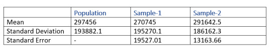
From the above table, the mean of the sample-2 which has a size of 200 entity is 291642.5 and the mean of the sample-1 is 270745. From this result, it is clear that sample-2 is better representative of the volume as compared to sample-1

            Similarly, when we take a look at the standard error, sample-2 is lesser as compared to sample-1. Which means that the sample-2 is more likely to be closer to the volume.

Population Distribution.

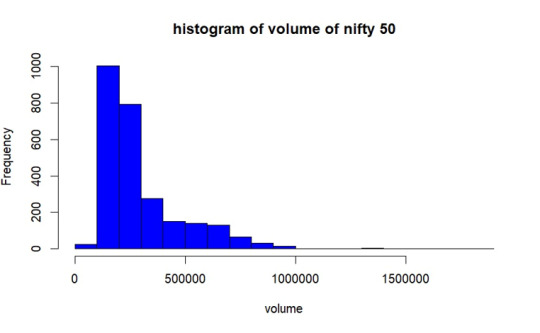
As per the graph, In most of the days from the year 2017 to 2023 December volume of trading of NIFTY50 was between 1lakh- 2.8lakhs.

Sample Selection

We are taking 2 sample set having 100 and 200 of size respectively without replacement. Then we obtained mean, standard deviation and standard error of both of the samples.

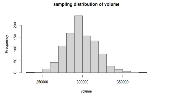
Sampling Distribution of Sample- 1

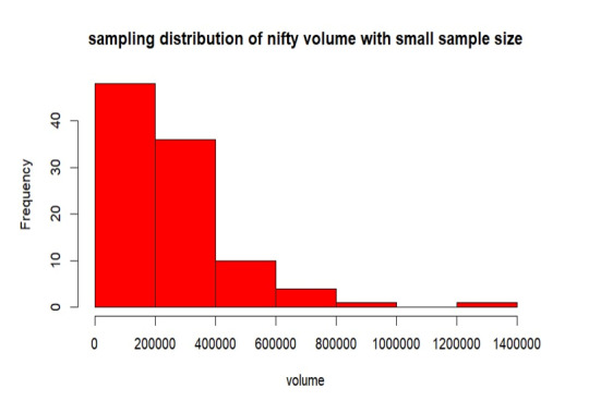
From the above graph, the samples are mostly between 0 to 2 lakhs of volume. Also, the samples are less distributed throughout the population. The mean is 270745, standard deviation is 195270.5 and the standard error of sampling is 19527.01.

Sampling Distribution of Sample- 2

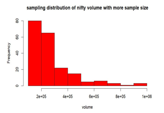
From the above graph, the samples are mostly between 0 to 2 lakhs of volume. Also, the samples are more distributed than the sample-1 throughout the volume. The mean is 291642.5, standard deviation is 186162.3 and the standard error of sampling is 13163.66.

Replication of Sample- 1

Here, we are duplicating the mean of every sample combination while taking into account every conceivable sample set from our volume. This suggests that the sample size is growing in this instance since the sample means follow the normal distribution according to the central limit theorem.

As per the above graph, it is clear that means of sample sets which we have replicated follows the normal distribution, from the graph the mean is around 3 lakhs which is approximately equals to our true volume mean 297456 which we have already calculated.

Conclusion

In the observed trading volume range of 2 lakhs to 3 lakhs, increasing the sample size led to a decrease in standard error. The sample mean converges to the true volume mean as sample size increases, according to this trend. Interestingly, the resulting sample distribution closely resembles the population when the sample mean is duplicated. The mean produced by this replication process is significantly more similar to the population mean, confirming the central limit theorem's validity in describing the real features of the trade volume.

[listtodatause]

From List to Data: A Beginner’s Guide to Data Transformation

In today’s data-driven world, transforming raw information into structured formats is a critical skill. One common task in data processing is converting a list—a simple, unstructured sequence of values—into structured data that can be analyzed, visualized, or stored. A “list” might be a shopping list, a sequence of names, or numbers collected from user inputs. “Data,” in contrast, refers to a structured format such as a table, database, or dataset. The goal of transforming a list to data is to make it usable for insights, automation, or further manipulation. Understanding this process helps beginners make sense of how information is organized in software systems, spreadsheets, or databases. It’s not just a programming task—it’s a foundational part of digital literacy.

Why Converting Lists to Data Matters

Lists are everywhere: in text files, spreadsheets, form submissions, or even copied from emails. But these lists often need structure before they can be used. Structured data can be sorted, filtered, analyzed, or even turned into charts. For example, if you receive a list of customer names and purchases, it’s just raw text until it’s organized into phone number data and columns—where each row is a customer and each column is a data point like name, item, or price. Without this transformation, automation tools, machine learning models, or even basic Excel functions can’t work effectively. Converting lists to structured data enables better decisions, reporting, and scaling of workflows.

Simple Tools for List-to-Data Conversion

You don’t need to be a coder to transform lists into data. Tools like Microsoft Excel, Google Sheets, or Notepad++ make this easy. For example, using the "Text to Columns" feature in Excel, you can split list items into cells. In Google Sheets, functions like SPLIT() and ARRAYFORMULA() help break down and reorganize text. Online tools like CSV converters also turn lists into structured CSV files. These steps make it easier for users to handle raw data without complex scripts. Beginners can start with drag-and-drop interfaces and learn basic data formatting.

Moving Beyond Basics: Automation with Python and Scripts

Once you’re comfortable with basic tools, learning to automate list-to-data conversions with scripting languages like Python is a powerful next step. Python libraries such as pandas make it simple to import a list from a file and convert it into a DataFrame—a table-like data structure. For example, if you have a list stored in a .txt file, Python can read it, parse it using string functions, and format it into rows and columns automatically. This is especially useful when handling large or repetitive data. Automating the process not only saves time but also reduces human error. It opens the door to building entire data pipelines, integrating APIs, or performing advanced analysis.

[advancedexcelinstitute]

A Beginner’s Guide to NVH Testing in India’s Automotive Industry

In today’s fast-paced world of data analytics, staying relevant means knowing how to turn raw data into smart decisions—and fast. Sure, tools like Python, SQL, and Power BI are gaining popularity, but if there’s one tool that still stands strong in 2025, it’s Microsoft Excel.

Whether you’re just starting out or you’ve been crunching numbers for years, Excel for data analyst roles remains one of the most practical and in-demand skills. It strikes that perfect balance between simplicity and capability, making it the go-to for countless data tasks.

In this post, we’ll look at why Excel isn’t going anywhere, the most valuable Excel job skills right now, and how you can sharpen your expertise to keep up with the latest demands in data analytics.

The Modern-Day Data Analyst: More Than Just a Number Cruncher

Back in the day, data analysts were mostly behind the scenes—collecting numbers, making charts, and maybe sending the occasional report. Fast forward to 2025, and their role is far more central. Today’s analysts are storytellers, business advisors, and problem solvers.

Here’s what a typical day might include:

Pulling raw data from different platforms (think CRMs, ERPs, databases, web analytics tools)

Cleaning and organizing that data so it actually makes sense

Analyzing trends to help forecast what’s coming next

Creating reports and dashboards that communicate findings clearly

Presenting insights to decision-makers in a way that drives action

And you guessed it—Excel shows up in almost every one of these steps.

Why Excel Still Matters (a Lot)

Some might argue that Excel is “old-school,” but here’s the reality: it’s still everywhere. And for good reason.

1. It’s Familiar to Everyone

From finance teams to marketing departments, most professionals have at least a basic grasp of Excel. That makes collaboration easy—no need to explain a tool everyone’s already using.

2. Quick Results, No Coding Required

Need to filter a dataset or run a few calculations? You can do it in Excel in minutes. It’s great for ad-hoc analysis where speed matters and there’s no time to build complex code.

3. Plays Nice with Other Tools

Excel isn’t an island. It connects smoothly with SQL databases, Google Analytics, Power BI, and even Python. Power Query is especially useful when pulling in and reshaping data from different sources.

4. It’s on Every Work Computer

You don’t need to install anything or get IT involved. Excel is ready to go on pretty much every company laptop, which makes it incredibly convenient.

Top Excel Skills Every Data Analyst Needs in 2025

To really stand out, you’ll want to move past the basics. Employers today expect you to do more than just sum a column or build a pie chart. Here’s where to focus your energy:

1. Data Cleaning and Transformation

Use functions like CLEAN(), TRIM(), and Text to Columns to fix messy data.

Power Query is a game-changer—it lets you clean, merge, and reshape large datasets without writing a line of code.

2. Advanced Formulas

Learn how to use INDEX, MATCH, XLOOKUP, IFERROR, and dynamic arrays. These help you build smarter, more flexible spreadsheets.

Nesting formulas (formulas within formulas) is super helpful for building logic into your models.

3. PivotTables and PivotCharts

Still one of the fastest ways to analyze large data sets.

Great for grouping, summarizing, and drilling into data—all without writing any SQL.

4. Power Query and Power Pivot

These tools turn Excel into a mini-BI platform.

You can pull in data from multiple tables, define relationships, and use DAX for more advanced calculations.

5. Interactive Dashboards

Combine charts, slicers, and conditional formatting to build dashboards that update as data changes.

Form controls (like drop-downs or sliders) add a professional touch.

6. Automation with Macros and VBA

Automate tasks like data formatting, report generation, and file creation.

Even basic VBA scripts can save hours each week on repetitive tasks.

Real-World Excel Use Cases That Still Matter

Let’s get practical. Here’s how Excel is still making an impact across industries:

Sales & Marketing: Track campaign performance, customer engagement, and conversion rates—all in a single dashboard.

Finance: Build cash flow models, scenario forecasts, and budget reports that help CFOs make data-driven calls.

Healthcare: Monitor key performance indicators like patient wait times or readmission rates.

Logistics: Analyze delivery times, shipping costs, and supplier performance to streamline operations.

These aren’t theoretical use cases—they’re actual day-to-day tasks being done in Excel right now.

Excel vs. Other Tools

Let’s be real: no single tool does it all. Excel fits into a broader ecosystem of data tools. Here’s a quick breakdown:TaskBest ToolHow Excel ContributesQuick AnalysisExcelFast and easy to useDashboardsPower BI / TableauExcel dashboards are perfect for internal or lightweight reportsData CleaningSQL / Power QueryExcel connects and transforms with Power QueryBig DataPython / RUse Excel for summary views and visualizations of Python output

Excel’s strength lies in how easily it fits into your workflow—even when you’re working with more advanced tools.

How to Get Better at Excel in 2025

If you’re serious about leveling up, here’s how to grow your skills:

1. Take a Course That Focuses on Analytics

Pick one that emphasizes real business problems and gives you projects to work on. Case studies are gold.

2. Practice on Real Data

Websites like Kaggle, data.gov, or even your company’s historical data (with permission, of course) are great places to start.

3. Learn Keyboard Shortcuts

You’ll work faster and feel more confident. Start with common ones like Ctrl + Shift + L for filters or Alt + = for autosum.

4. Dive into Power Query and Power Pivot

Once you get the hang of them, you’ll wonder how you ever worked without them.

5. Build Mini Projects

Create dashboards or models that solve specific business problems—like tracking customer churn or sales performance. These can become portfolio pieces for your next job interview.

Conclusion

Excel isn’t going anywhere. It’s deeply woven into how businesses run, and in 2025, it’s still one of the best tools in a data analyst’s toolkit. It might not be as flashy as Python or as powerful as Tableau, but it gets the job done—and done well.

If you’re aiming to future-proof your career, investing in advanced Excel job skills is a smart move. From dashboards to data modeling, the possibilities are endless. And when paired with other tools, Excel helps you deliver even more value to your team.

So keep practicing, keep building, and remember—being great at Excel can set you apart in the data world.

FAQs

Is Excel still worth learning for data analysis in 2025?Yes! Excel remains one of the top skills hiring managers look for in data analyst roles. It’s everywhere—from startups to large enterprises.

What are the most useful Excel features for analysts? Advanced formulas, PivotTables, Power Query, Power Pivot, and dashboard design are the big ones. Knowing VBA is a bonus.

Can Excel handle big datasets?To an extent. While Excel has limits, features like Power Query and Power Pivot help it manage more data than it could in the past. For really massive data, combine it with tools like SQL or Power BI.

Should I learn Excel or Python?Both. Excel is great for quick analysis and reporting. Python is better for automation, data science, and machine learning. Together, they’re a powerful combo.

How can I show off my Excel skills to employers? Create dashboards or reports based on real data and include them in a portfolio. Show how you used Excel to solve actual business problems on your resume.

[phoebewang]

LASSO

The dataset was split into training (70%) and testing (30%) subsets.

MSE:

training data MSE=0.17315418324424045 ; test data MSE =0.1702171216510316

R-squared:

training data R-square=0.088021944671551 ; test data R-square = 0.08363901452881095

This graph shows how the mean squared error (MSE) varies with the regularization penalty term (𝛼) during 10-fold cross-validation. Each dotted line indicates the validation error from a single fold, whereas the solid black line is the average MSE over all folds. The vertical dashed line represents the value of 𝛼 that minimized the average MSE, indicating the model's optimal balance of complexity and prediction accuracy.

As 𝛼 decreases (from left to right on the x-axis, as demonstrated by rising −log 10 (α)), the model becomes less regularized, enabling additional predictors to enter. The average MSE initially fell, indicating that adding more variables enhanced the model's performance. However, beyond a certain point, the average MSE smoothed out and slightly rose, indicating possible overfitting when too many predictors were added.

The minimal point on the curve, shown by the vertical dashed line, is the ideal regularization level utilized in the final model. At this phase, the model preserved the subset of variables that had the lowest cross-validated prediction error. The relatively flat tail of the curve indicates that the model's performance was constant throughout a variety of adjacent alpha values, lending confidence to the chosen predictors.

Overall, this graph shows which predictor variables survived after the penalty was applied. Those who survived would have a strong predictive power for the outcome.

This graph shows the coefficient change for each predictor variable in the Lasso regression model based on the regularization penalty term, represented as −log 10(α). As the penalty moves rightward, additional coefficients enter the model and increase in size, demonstrating their importance in predicting drinking frequency.

As shown by the vertical dashed line (alpha CV) representing the optimal alpha level, numerous variables exhibit non-zero coefficients, indicating that they were maintained in the final model as significant predictors of drinking frequency.

The orange and blue line, specifically, suggests a strong prediction pattern of the drinking frequency since they grow rapidly and dominate the model at low regularization levels.

Some other coefficients stay close to 0 or equal to zero across most alpha values, indicating that they were either removed or had few impacts on the final model. The coefficients' stability as regularization lowers indicates that certain predictors have persistent significance regardless of the degree of shrinkage.

Code: A lasso regression analysis was used to determine which factors from a pool of 16 demographic and behavioral predictors best predicted drinking frequency among adult respondents in the NESARC dataset. To ensure that regression coefficients are comparable, all predictors were normalized with a mean of zero and a standard deviation of one. The dataset was divided into training (70%), and testing (30%) sections. The training data was used to apply a lasso regression model with 10-fold cross-validation using Python's LassoCV function. The penalty term (𝛼) was automatically tweaked to reduce cross-validated prediction error.

import pandas as pd import numpy as np import matplotlib.pylab as plt from sklearn.model_selection import train_test_split from sklearn.linear_model import LassoLarsCV

#Load the dataset

data = pd.read_csv("_358bd6a81b9045d95c894acf255c696a_nesarc_pds.csv")

#Data Management

#Subset relevant columns

cols = ['S2AQ21B', 'AGE', 'SEX', 'S1Q7A11', 'FMARITAL','S1Q7A1','S1Q7A8','S1Q7A9','S1Q7A2','S1Q7A3','S1Q1D4','S1Q1D3', 'S1Q1D2','S1Q1D1','ADULTCH','OTHREL','S1Q24LB'] data = data[cols]

#Replace blanks and invalid codes

data['S2AQ21B'] = data['S2AQ21B'].replace([' ', 98, 99, 'BL'], pd.NA)

#Drop rows with missing target values

data = data.dropna(subset=['S2AQ21B'])

#Convert to numeric and recode binary target

data['S2AQ21B'] = data['S2AQ21B'].astype(int) data['DRINKFREQ'] = data['S2AQ21B'].apply(lambda x: 1 if x in [1, 2, 3, 4] else 0)

#select predictor variables and target variable as separate data sets

predvar= data[['AGE', 'SEX', 'S1Q7A11', 'FMARITAL', 'S1Q7A1','S1Q7A8','S1Q7A9','S1Q7A2','S1Q7A3','S1Q1D4','S1Q1D3', 'S1Q1D2','S1Q1D1','ADULTCH','OTHREL','S1Q24LB']]

target = data['DRINKFREQ']

#standardize predictors to have mean=0 and sd=1

predictors=predvar.copy() from sklearn import preprocessing predictors['AGE']=preprocessing.scale(predictors['AGE'].astype('float64')) predictors['SEX']=preprocessing.scale(predictors['SEX'].astype('float64')) predictors['S1Q7A11']=preprocessing.scale(predictors['S1Q7A11'].astype('float64')) predictors['FMARITAL']=preprocessing.scale(predictors['FMARITAL'].astype('float64')) predictors['S1Q7A1']=preprocessing.scale(predictors['S1Q7A1'].astype('float64')) predictors['S1Q7A8']=preprocessing.scale(predictors['S1Q7A8'].astype('float64')) predictors['S1Q7A9']=preprocessing.scale(predictors['S1Q7A9'].astype('float64')) predictors['S1Q7A2']=preprocessing.scale(predictors['S1Q7A2'].astype('float64')) predictors['S1Q7A3']=preprocessing.scale(predictors['S1Q7A3'].astype('float64')) predictors['S1Q1D4']=preprocessing.scale(predictors['S1Q1D4'].astype('float64')) predictors['S1Q1D3']=preprocessing.scale(predictors['S1Q1D3'].astype('float64')) predictors['S1Q1D2']=preprocessing.scale(predictors['S1Q1D2'].astype('float64')) predictors['S1Q1D1']=preprocessing.scale(predictors['S1Q1D1'].astype('float64')) predictors['ADULTCH']=preprocessing.scale(predictors['ADULTCH'].astype('float64')) predictors['OTHREL']=preprocessing.scale(predictors['OTHREL'].astype('float64')) predictors['S1Q24LB']=preprocessing.scale(predictors['S1Q24LB'].astype('float64'))

#split data into train and test sets

pred_train, pred_test, tar_train, tar_test = train_test_split(predictors, target, test_size=.3, random_state=123)

#specify the lasso regression model

from sklearn.linear_model import LassoCV lasso = LassoCV(cv=10, random_state=0).fit(pred_train, tar_train)

#print variable names and regression coefficients

dict(zip(predictors.columns, model.coef_))

--------------

#plot coefficient progression

from sklearn.linear_model import lasso_path

#Compute the full coefficient path

alphas_lasso, coefs_lasso, _ = lasso_path(pred_train, tar_train)

#Plot the coefficient paths

plt.figure(figsize=(10, 6)) neg_log_alphas = -np.log10(alphas_lasso) for coef in coefs_lasso: plt.plot(neg_log_alphas, coef)

plt.axvline(-np.log10(lasso.alpha_), color='k', linestyle='--', label='alpha (CV)') plt.xlabel('-log10(alpha)') plt.ylabel('Coefficients') plt.title('Lasso Paths: Coefficient Progression') plt.legend() plt.tight_layout() plt.show()

-------------------

#plot mean square error for each fold

m_log_alphascv = -np.log10(lasso.alphas_) plt.figure(figsize=(8, 5)) plt.plot(m_log_alphascv, lasso.mse_path_, ':') plt.plot(m_log_alphascv, lasso.mse_path_.mean(axis=-1), 'k', label='Average across the folds', linewidth=2) plt.axvline(-np.log10(lasso.alpha_), linestyle='--', color='k', label='alpha CV') plt.legend() plt.xlabel('-log(alpha)') plt.ylabel('Mean squared error') plt.title('Mean squared error on each fold')

----------------------

#MSE from training and test data

from sklearn.metrics import mean_squared_error train_error = mean_squared_error(tar_train, model.predict(pred_train)) test_error = mean_squared_error(tar_test, model.predict(pred_test)) print ('training data MSE') print(train_error) print ('test data MSE') print(test_error)

----------------------

#R-square from training and test data

rsquared_train=model.score(pred_train,tar_train) rsquared_test=model.score(pred_test,tar_test) print ('training data R-square') print(rsquared_train) print ('test data R-square') print(rsquared_test)

[tia003]

How do you handle missing data in a dataset?

Handling missing data is a crucial step in data preprocessing, as incomplete datasets can lead to biased or inaccurate analysis. There are several techniques to deal with missing values, depending on the nature of the data and the extent of missingness.

1. Identifying Missing Data Before handling missing values, it is important to detect them using functions like .isnull() in Python’s Pandas library. Understanding the pattern of missing data (random or systematic) helps in selecting the best strategy.

2. Removing Missing Data

If the missing values are minimal (e.g., less than 5% of the dataset), you can remove the affected rows using dropna().

If entire columns contain a significant amount of missing data, they may be dropped if they are not crucial for analysis.

3. Imputation Techniques

Mean/Median/Mode Imputation: For numerical data, replacing missing values with the mean, median, or mode of the column ensures continuity in the dataset.

Forward or Backward Fill: For time-series data, forward filling (ffill()) or backward filling (bfill()) propagates values from previous or next entries.

Interpolation: Using methods like linear or polynomial interpolation estimates missing values based on trends in the dataset.

Predictive Modeling: More advanced techniques use machine learning models like K-Nearest Neighbors (KNN) or regression to predict and fill missing values.

4. Using Algorithms That Handle Missing Data Some machine learning algorithms, like decision trees and random forests, can handle missing values internally without imputation.

By applying these techniques, data quality is improved, leading to more accurate insights. To master such data preprocessing techniques, consider enrolling in the best data analytics certification, which provides hands-on training in handling real-world datasets.

[fromdevcom]

Pandas DataFrame Cleanup: Master the Art of Dropping Columns Data cleaning and preprocessing are crucial steps in any data analysis project. When working with pandas DataFrames in Python, you'll often encounter situations where you need to remove unnecessary columns to streamline your dataset. In this comprehensive guide, we'll explore various methods to drop columns in pandas, complete with practical examples and best practices. Understanding the Basics of Column Dropping Before diving into the methods, let's understand why we might need to drop columns: Remove irrelevant features that don't contribute to analysis Eliminate duplicate or redundant information Clean up data before model training Reduce memory usage for large datasets Method 1: Using drop() - The Most Common Approach The drop() method is the most straightforward way to remove columns from a DataFrame. Here's how to use it: pythonCopyimport pandas as pd # Create a sample DataFrame df = pd.DataFrame( 'name': ['John', 'Alice', 'Bob'], 'age': [25, 30, 35], 'city': ['New York', 'London', 'Paris'], 'temp_col': [1, 2, 3] ) # Drop a single column df = df.drop('temp_col', axis=1) # Drop multiple columns df = df.drop(['city', 'age'], axis=1) The axis=1 parameter indicates we're dropping columns (not rows). Remember that drop() returns a new DataFrame by default, so we need to reassign it or use inplace=True. Method 2: Using del Statement - The Quick Solution For quick, permanent column removal, you can use Python's del statement: pythonCopy# Delete a column using del del df['temp_col'] Note that this method modifies the DataFrame directly and cannot be undone. Use it with caution! Method 3: Drop Columns Using pop() - Remove and Return The pop() method removes a column and returns it, which can be useful when you want to store the removed column: pythonCopy# Remove and store a column removed_column = df.pop('temp_col') Advanced Column Dropping Techniques Dropping Multiple Columns with Pattern Matching Sometimes you need to drop columns based on patterns in their names: pythonCopy# Drop columns that start with 'temp_' df = df.drop(columns=df.filter(regex='^temp_').columns) # Drop columns that contain certain text df = df.drop(columns=df.filter(like='unused').columns) Conditional Column Dropping You might want to drop columns based on certain conditions: pythonCopy# Drop columns with more than 50% missing values threshold = len(df) * 0.5 df = df.dropna(axis=1, thresh=threshold) # Drop columns of specific data types df = df.select_dtypes(exclude=['object']) Best Practices for Dropping Columns Make a Copy First pythonCopydf_clean = df.copy() df_clean = df_clean.drop('column_name', axis=1) Use Column Lists for Multiple Drops pythonCopycolumns_to_drop = ['col1', 'col2', 'col3'] df = df.drop(columns=columns_to_drop) Error Handling pythonCopytry: df = df.drop('non_existent_column', axis=1) except KeyError: print("Column not found in DataFrame") Performance Considerations When working with large datasets, consider these performance tips: Use inplace=True to avoid creating copies: pythonCopydf.drop('column_name', axis=1, inplace=True) Drop multiple columns at once rather than one by one: pythonCopy# More efficient df.drop(['col1', 'col2', 'col3'], axis=1, inplace=True) # Less efficient df.drop('col1', axis=1, inplace=True) df.drop('col2', axis=1, inplace=True) df.drop('col3', axis=1, inplace=True) Common Pitfalls and Solutions Dropping Non-existent Columns pythonCopy# Use errors='ignore' to skip non-existent columns df = df.drop('missing_column', axis=1, errors='ignore') Chain Operations Safely pythonCopy# Use method chaining carefully df = (df.drop('col1', axis=1) .drop('col2', axis=1) .reset_index(drop=True)) Real-World Applications Let's look at a practical example of cleaning a dataset: pythonCopy# Load a messy dataset df = pd.read_csv('raw_data.csv')

# Clean up the DataFrame df_clean = (df.drop(columns=['unnamed_column', 'duplicate_info']) # Remove unnecessary columns .drop(columns=df.filter(regex='^temp_').columns) # Remove temporary columns .drop(columns=df.columns[df.isna().sum() > len(df)*0.5]) # Remove columns with >50% missing values ) Integration with Data Science Workflows When preparing data for machine learning: pythonCopy# Drop target variable from features X = df.drop('target_variable', axis=1) y = df['target_variable'] # Drop non-numeric columns for certain algorithms X = X.select_dtypes(include=['float64', 'int64']) Conclusion Mastering column dropping in pandas is essential for effective data preprocessing. Whether you're using the simple drop() method or implementing more complex pattern-based dropping, understanding these techniques will make your data cleaning process more efficient and reliable. Remember to always consider your specific use case when choosing a method, and don't forget to make backups of important data before making permanent changes to your DataFrame. Now you're equipped with all the knowledge needed to effectively manage columns in your pandas DataFrames. Happy data cleaning!

[datasciencewithmohsin]

Feature Engineering in Machine Learning: A Beginner's Guide

Feature Engineering in Machine Learning: A Beginner's Guide

Feature engineering is one of the most critical aspects of machine learning and data science. It involves preparing raw data, transforming it into meaningful features, and optimizing it for use in machine learning models. Simply put, it’s all about making your data as informative and useful as possible.

In this article, we’re going to focus on feature transformation, a specific type of feature engineering. We’ll cover its types in detail, including:

1. Missing Value Imputation

2. Handling Categorical Data

3. Outlier Detection

4. Feature Scaling

Each topic will be explained in a simple and beginner-friendly way, followed by Python code examples so you can implement these techniques in your projects.

What is Feature Transformation?

Feature transformation is the process of modifying or optimizing features in a dataset. Why? Because raw data isn’t always machine-learning-friendly. For example:

Missing data can confuse your model.

Categorical data (like colors or cities) needs to be converted into numbers.

Outliers can skew your model’s predictions.

Different scales of features (e.g., age vs. income) can mess up distance-based algorithms like k-NN.

1. Missing Value Imputation

Missing values are common in datasets. They can happen due to various reasons: incomplete surveys, technical issues, or human errors. But machine learning models can’t handle missing data directly, so we need to fill or "impute" these gaps.

Techniques for Missing Value Imputation

1. Dropping Missing Values: This is the simplest method, but it’s risky. If you drop too many rows or columns, you might lose important information.

2. Mean, Median, or Mode Imputation: Replace missing values with the column’s mean (average), median (middle value), or mode (most frequent value).

3. Predictive Imputation: Use a model to predict the missing values based on other features.

Python Code Example:

import pandas as pd

from sklearn.impute import SimpleImputer

# Example dataset

data = {'Age': [25, 30, None, 22, 28], 'Salary': [50000, None, 55000, 52000, 58000]}

df = pd.DataFrame(data)

# Mean imputation

imputer = SimpleImputer(strategy='mean')

df['Age'] = imputer.fit_transform(df[['Age']])

df['Salary'] = imputer.fit_transform(df[['Salary']])

print("After Missing Value Imputation:\n", df)

Key Points:

Use mean/median imputation for numeric data.

Use mode imputation for categorical data.

Always check how much data is missing—if it’s too much, dropping rows might be better.

2. Handling Categorical Data

Categorical data is everywhere: gender, city names, product types. But machine learning algorithms require numerical inputs, so you’ll need to convert these categories into numbers.

Techniques for Handling Categorical Data

1. Label Encoding: Assign a unique number to each category. For example, Male = 0, Female = 1.

2. One-Hot Encoding: Create separate binary columns for each category. For instance, a “City” column with values [New York, Paris] becomes two columns: City_New York and City_Paris.

3. Frequency Encoding: Replace categories with their occurrence frequency.

Python Code Example:

from sklearn.preprocessing import LabelEncoder

import pandas as pd

# Example dataset

data = {'City': ['New York', 'London', 'Paris', 'New York', 'Paris']}

df = pd.DataFrame(data)

# Label Encoding

label_encoder = LabelEncoder()

df['City_LabelEncoded'] = label_encoder.fit_transform(df['City'])

# One-Hot Encoding

df_onehot = pd.get_dummies(df['City'], prefix='City')

print("Label Encoded Data:\n", df)

print("\nOne-Hot Encoded Data:\n", df_onehot)

Key Points:

Use label encoding when categories have an order (e.g., Low, Medium, High).

Use one-hot encoding for non-ordered categories like city names.

For datasets with many categories, one-hot encoding can increase complexity.

3. Outlier Detection

Outliers are extreme data points that lie far outside the normal range of values. They can distort your analysis and negatively affect model performance.

Techniques for Outlier Detection

1. Interquartile Range (IQR): Identify outliers based on the middle 50% of the data (the interquartile range).

IQR = Q3 - Q1

[Q1 - 1.5 \times IQR, Q3 + 1.5 \times IQR]

2. Z-Score: Measures how many standard deviations a data point is from the mean. Values with Z-scores > 3 or < -3 are considered outliers.

Python Code Example (IQR Method):

import pandas as pd

# Example dataset

data = {'Values': [12, 14, 18, 22, 25, 28, 32, 95, 100]}

df = pd.DataFrame(data)

# Calculate IQR

Q1 = df['Values'].quantile(0.25)

Q3 = df['Values'].quantile(0.75)

IQR = Q3 - Q1

# Define bounds

lower_bound = Q1 - 1.5 * IQR

upper_bound = Q3 + 1.5 * IQR

# Identify and remove outliers

outliers = df[(df['Values'] < lower_bound) | (df['Values'] > upper_bound)]

print("Outliers:\n", outliers)

filtered_data = df[(df['Values'] >= lower_bound) & (df['Values'] <= upper_bound)]

print("Filtered Data:\n", filtered_data)

Key Points:

Always understand why outliers exist before removing them.

Visualization (like box plots) can help detect outliers more easily.

4. Feature Scaling

Feature scaling ensures that all numerical features are on the same scale. This is especially important for distance-based models like k-Nearest Neighbors (k-NN) or Support Vector Machines (SVM).

Techniques for Feature Scaling

1. Min-Max Scaling: Scales features to a range of [0, 1].

X' = \frac{X - X_{\text{min}}}{X_{\text{max}} - X_{\text{min}}}

2. Standardization (Z-Score Scaling): Centers data around zero with a standard deviation of 1.

X' = \frac{X - \mu}{\sigma}

3. Robust Scaling: Uses the median and IQR, making it robust to outliers.

Python Code Example:

from sklearn.preprocessing import MinMaxScaler, StandardScaler

import pandas as pd

# Example dataset

data = {'Age': [25, 30, 35, 40, 45], 'Salary': [20000, 30000, 40000, 50000, 60000]}

df = pd.DataFrame(data)

# Min-Max Scaling

scaler = MinMaxScaler()

df_minmax = pd.DataFrame(scaler.fit_transform(df), columns=df.columns)

# Standardization

scaler = StandardScaler()

df_standard = pd.DataFrame(scaler.fit_transform(df), columns=df.columns)

print("Min-Max Scaled Data:\n", df_minmax)

print("\nStandardized Data:\n", df_standard)

Key Points:

Use Min-Max Scaling for algorithms like k-NN and neural networks.

Use Standardization for algorithms that assume normal distributions.

Use Robust Scaling when your data has outliers.

Final Thoughts

Feature transformation is a vital part of the data preprocessing pipeline. By properly imputing missing values, encoding categorical data, handling outliers, and scaling features, you can dramatically improve the performance of your machine learning models.

Summary:

Missing value imputation fills gaps in your data.

Handling categorical data converts non-numeric features into numerical ones.

Outlier detection ensures your dataset isn’t skewed by extreme values.

Feature scaling standardizes feature ranges for better model performance.

Mastering these techniques will help you build better, more reliable machine learning models.

[abhinav3045]

About

Course

Basic Stats

Machine Learning

Software Tutorials

Tools

K-Means Clustering in Python: Step-by-Step Example

by Zach BobbittPosted on August 31, 2022

One of the most common clustering algorithms in machine learning is known as k-means clustering.

K-means clustering is a technique in which we place each observation in a dataset into one of K clusters.

The end goal is to have K clusters in which the observations within each cluster are quite similar to each other while the observations in different clusters are quite different from each other.

In practice, we use the following steps to perform K-means clustering:

1. Choose a value for K.

First, we must decide how many clusters we’d like to identify in the data. Often we have to simply test several different values for K and analyze the results to see which number of clusters seems to make the most sense for a given problem.

2. Randomly assign each observation to an initial cluster, from 1 to K.

3. Perform the following procedure until the cluster assignments stop changing.

For each of the K clusters, compute the cluster centroid. This is simply the vector of the p feature means for the observations in the kth cluster.

Assign each observation to the cluster whose centroid is closest. Here, closest is defined using Euclidean distance.

The following step-by-step example shows how to perform k-means clustering in Python by using the KMeans function from the sklearn module.

Step 1: Import Necessary Modules

First, we’ll import all of the modules that we will need to perform k-means clustering:import pandas as pd import numpy as np import matplotlib.pyplot as plt from sklearn.cluster import KMeans from sklearn.preprocessing import StandardScaler

Step 2: Create the DataFrame

Next, we’ll create a DataFrame that contains the following three variables for 20 different basketball players:

points

assists

rebounds

The following code shows how to create this pandas DataFrame:#create DataFrame df = pd.DataFrame({'points': [18, np.nan, 19, 14, 14, 11, 20, 28, 30, 31, 35, 33, 29, 25, 25, 27, 29, 30, 19, 23], 'assists': [3, 3, 4, 5, 4, 7, 8, 7, 6, 9, 12, 14, np.nan, 9, 4, 3, 4, 12, 15, 11], 'rebounds': [15, 14, 14, 10, 8, 14, 13, 9, 5, 4, 11, 6, 5, 5, 3, 8, 12, 7, 6, 5]}) #view first five rows of DataFrame print(df.head()) points assists rebounds 0 18.0 3.0 15 1 NaN 3.0 14 2 19.0 4.0 14 3 14.0 5.0 10 4 14.0 4.0 8

We will use k-means clustering to group together players that are similar based on these three metrics.

Step 3: Clean & Prep the DataFrame

Next, we’ll perform the following steps:

Use dropna() to drop rows with NaN values in any column

Use StandardScaler() to scale each variable to have a mean of 0 and a standard deviation of 1

The following code shows how to do so:#drop rows with NA values in any columns df = df.dropna() #create scaled DataFrame where each variable has mean of 0 and standard dev of 1 scaled_df = StandardScaler().fit_transform(df) #view first five rows of scaled DataFrame print(scaled_df[:5]) [[-0.86660275 -1.22683918 1.72722524] [-0.72081911 -0.96077767 1.45687694] [-1.44973731 -0.69471616 0.37548375] [-1.44973731 -0.96077767 -0.16521285] [-1.88708823 -0.16259314 1.45687694]]

Note: We use scaling so that each variable has equal importance when fitting the k-means algorithm. Otherwise, the variables with the widest ranges would have too much influence.

Step 4: Find the Optimal Number of Clusters

To perform k-means clustering in Python, we can use the KMeans function from the sklearn module.

This function uses the following basic syntax:

KMeans(init=’random’, n_clusters=8, n_init=10, random_state=None)

where:

init: Controls the initialization technique.

n_clusters: The number of clusters to place observations in.

n_init: The number of initializations to perform. The default is to run the k-means algorithm 10 times and return the one with the lowest SSE.

random_state: An integer value you can pick to make the results of the algorithm reproducible. 

The most important argument in this function is n_clusters, which specifies how many clusters to place the observations in.

However, we don’t know beforehand how many clusters is optimal so we must create a plot that displays the number of clusters along with the SSE (sum of squared errors) of the model.

Typically when we create this type of plot we look for an “elbow” where the sum of squares begins to “bend” or level off. This is typically the optimal number of clusters.

The following code shows how to create this type of plot that displays the number of clusters on the x-axis and the SSE on the y-axis:#initialize kmeans parameters kmeans_kwargs = { "init": "random", "n_init": 10, "random_state": 1, } #create list to hold SSE values for each k sse = [] for k in range(1, 11): kmeans = KMeans(n_clusters=k, **kmeans_kwargs) kmeans.fit(scaled_df) sse.append(kmeans.inertia_) #visualize results plt.plot(range(1, 11), sse) plt.xticks(range(1, 11)) plt.xlabel("Number of Clusters") plt.ylabel("SSE") plt.show()

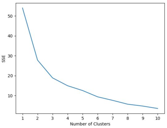
In this plot it appears that there is an elbow or “bend” at k = 3 clusters.

Thus, we will use 3 clusters when fitting our k-means clustering model in the next step.

Note: In the real-world, it’s recommended to use a combination of this plot along with domain expertise to pick how many clusters to use.

Step 5: Perform K-Means Clustering with Optimal K

The following code shows how to perform k-means clustering on the dataset using the optimal value for k of 3:#instantiate the k-means class, using optimal number of clusters kmeans = KMeans(init="random", n_clusters=3, n_init=10, random_state=1) #fit k-means algorithm to data kmeans.fit(scaled_df) #view cluster assignments for each observation kmeans.labels_ array([1, 1, 1, 1, 1, 1, 2, 2, 0, 0, 0, 0, 2, 2, 2, 0, 0, 0])

The resulting array shows the cluster assignments for each observation in the DataFrame.

To make these results easier to interpret, we can add a column to the DataFrame that shows the cluster assignment of each player:#append cluster assingments to original DataFrame df['cluster'] = kmeans.labels_ #view updated DataFrame print(df) points assists rebounds cluster 0 18.0 3.0 15 1 2 19.0 4.0 14 1 3 14.0 5.0 10 1 4 14.0 4.0 8 1 5 11.0 7.0 14 1 6 20.0 8.0 13 1 7 28.0 7.0 9 2 8 30.0 6.0 5 2 9 31.0 9.0 4 0 10 35.0 12.0 11 0 11 33.0 14.0 6 0 13 25.0 9.0 5 0 14 25.0 4.0 3 2 15 27.0 3.0 8 2 16 29.0 4.0 12 2 17 30.0 12.0 7 0 18 19.0 15.0 6 0 19 23.0 11.0 5 0

The cluster column contains a cluster number (0, 1, or 2) that each player was assigned to.

Players that belong to the same cluster have roughly similar values for the points, assists, and rebounds columns.

Note: You can find the complete documentation for the KMeans function from sklearn here.

Additional Resources

The following tutorials explain how to perform other common tasks in Python:

How to Perform Linear Regression in Python How to Perform Logistic Regression in Python How to Perform K-Fold Cross Validation in Python

[stockmarketanalysis]

📈 The Only Line Chart Guide You’ll Ever Need (With Real Examples from India)

Line charts, or line graphs, are among the simplest yet most powerful tools in the data visualization world. Whether you're tracking Nifty 50 trends, analyzing website traffic, or forecasting COVID-19 cases, the humble line chart has your back.

This guide dives deep into what line charts are, when to use them, how to build them with tools like Strike Money, and how to avoid common mistakes.

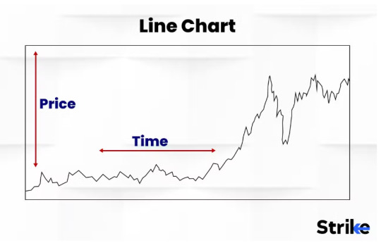
🔍 What Exactly Is a Line Chart and Why It’s Used Everywhere

A line chart is a graphical representation of data points connected by straight lines. It’s primarily used to show trends over time — ideal for time series data.

You’ll see line charts in:

Financial reports (like Sensex closing prices)

Health dashboards (like daily COVID-19 recoveries)

Marketing (like monthly traffic growth)

Scientific research (like temperature variations)

Why it matters: Humans are hardwired to spot patterns. Line graphs help us quickly identify spikes, dips, and trends without crunching numbers.

📊 Break It Down: Anatomy of a Line Chart

Before diving in, let’s decode the parts:

X-Axis: Represents time or categories (e.g., months, days)

Y-Axis: Shows the metric (e.g., stock price, temperature)

Data Points: Actual values plotted on the graph

Trend Line: Connects data points to show progression

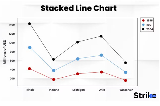
Multiple Lines: Used to compare multiple datasets (e.g., Reliance vs. Infosys stock)

Example: A line chart of Nifty 50 from Jan to Dec shows market recovery post COVID-19 waves — from under 12,000 in March 2020 to 18,000+ in 2021.

🧠 When Should You Use a Line Chart? Don’t Just Guess

Use a line chart when your data has a logical progression — especially over time.

✅ Best Use Cases:

Stock performance: e.g., tracking HDFC Bank stock price over 5 years

Economic trends: e.g., India’s GDP growth rate per quarter

Sales and revenue: e.g., monthly product sales

Social media engagement: e.g., follower count growth over time

💡Pro Tip: Avoid using line charts if your data isn’t continuous. For categories (like customer type or product type), use bar charts instead.

🚀 Want to Build a Line Chart? These Are the Tools You Need

There are several tools out there — from spreadsheets to data science libraries.

Here are the most used platforms:

1. Strike Money

A user-friendly Indian charting tool built for stock traders and financial analysts. Plot live stock trends, compare multiple equities, and use advanced indicators on interactive line graphs.

Example: Plot Infosys, TCS, and HCL Tech on one line chart to compare IT sector momentum.

2. Microsoft Excel / Google Sheets

Perfect for beginners and business users. Just insert your data and select “Insert Line Chart.”

3. Python (Matplotlib / Seaborn)

Ideal for data scientists and developers. Highly customizable, great for big datasets.import matplotlib.pyplot as plt plt.plot(dates, stock_prices) plt.title("Infosys Stock Over Time") plt.xlabel("Date") plt.ylabel("Price (INR)") plt.show()

4. Tableau / Power BI

Best for dashboards and presentations. Easy drag-and-drop interface for real-time visuals.

🧪 Step-by-Step: How to Create Line Charts Like a Pro

Let’s say you want to visualize Maruti Suzuki stock price in 2024.

In Strike Money:

Go to the charting dashboard

Type MARUTI in the ticker search

Select Line Chart from chart type dropdown

Customize time range (1 month to 5 years)

Add comparison lines or indicators as needed

In Google Sheets:

Enter dates in column A, prices in column B

Highlight data → Insert → Chart

Choose “Line Chart” under chart type

Style your chart (colors, labels)

Result? A clean, readable graph ready to share or embed.

🤔 Line Chart vs Bar Chart vs Scatter Plot — Which One Should You Use?

Choosing the right chart type is crucial for clear storytelling. Use Case Best Chart Trends over time Line Chart Comparing categories Bar Chart Correlation between variables Scatter Plot

Example: If you want to show how HDFC Bank’s price moved from Jan to March — line chart is perfect. If you want to compare Q4 revenue between HDFC, ICICI, and Axis — go with bar chart.

🎯 Follow These Best Practices for Better Line Charts

A good line chart is clear, accurate, and tells a story.

🔑 Design Tips:

Use consistent intervals on the X-axis

Avoid clutter: Limit to 3–4 lines max

Highlight key points with data labels

Always label axes and units

Use colors with purpose — not decoration

🛑 Avoid using 3D effects or unnecessary gridlines. It reduces readability.

📉 Case in Point: The RBI once published inflation trends without labeling the Y-axis units — leading to misinterpretation by media outlets.

🏦 Real Examples from Indian Stock Market That Use Line Charts

📈 Example 1: Nifty 50 Historical Line Chart

From 2018 to 2024, the Nifty 50 showed significant recovery post-pandemic. Line charts highlighted:

Crash during March 2020 (COVID panic)

Gradual recovery till late 2021

Volatility during global recession signals (2022–2023)

📈 Example 2: Reliance vs. Tata Motors (2023)

Using Strike Money, plotting these two giants shows:

Reliance remained flat post Q2 results

Tata Motors rose steadily due to strong EV sales

These comparisons are clearer on line charts than any table or bar chart.

❌ Don’t Make These Mistakes With Line Charts

Many beginners (and even analysts) misuse line graphs. Here’s what to avoid:

1. Inconsistent time intervals

Never mix weekly and monthly data on one line. It breaks flow and misleads.

2. Manipulated axes

Truncating the Y-axis can exaggerate or hide trends. Always start from zero unless context demands otherwise.

3. Too many lines

Four or more lines = spaghetti. It confuses more than it explains.

4. Unlabeled axes

Your audience shouldn’t guess what the graph means.

📚 What Research Says About Line Charts and Data Comprehension

Multiple studies back the effectiveness of line charts:

A 2019 MIT study found that line charts are the fastest chart type to interpret for time-based data.

In a Nielsen Norman Group UX test, 73% of users could accurately describe trends from line charts compared to only 45% from raw tables.

According to Google’s Data Visualization Guidelines, line charts are the default recommendation for dashboards involving time-based KPIs.

💡 How Line Charts Power Data Storytelling and Better Decisions

The real power of line charts isn’t just in their simplicity — it’s in the story they tell over time.

In business, a well-designed line chart can:

Justify a new budget (e.g., marketing ROI growth)

Show underperformance (e.g., product sales dip)

Communicate urgency (e.g., rising churn rate)

Inspire confidence (e.g., growing user base)

Example: During India’s COVID-19 second wave, the Ministry of Health used line charts daily to show rising cases. It informed lockdown decisions and public behavior.

In finance, line graphs of stock volatility are used to guide investment strategy.

🧭 Wrapping Up: Your Takeaway from This Line Chart Guide

To recap:

Use line charts to show trends over time.

Choose the right tool like Strike Money, Excel, or Python.

Keep it simple, clear, and focused.

Avoid clutter and misleading designs.

Use real-world data storytelling to drive impact.

Whether you're a marketer, analyst, or trader, mastering line charts will level up your data game.

👇 Ready to Create Stunning Line Charts?

Explore Strike Money — a powerful charting tool for Indian market data. Build, customize, and analyze stock trends like a pro — no code needed.

Line charts aren't just visuals. They're stories. And every dataset has one worth telling.

[govindhtech]

BigQuery DataFrames Generative AI Goldmines!

Generative AI in BigQuery DataFrames turns customer feedback into opportunities

To run a successful business, you must understand your customers’ needs and learn from their feedback. However, extracting actionable information from customer feedback is difficult. Examining and categorizing feedback can help you identify your customers’ product pain points, but it can become difficult and time-consuming as feedback grows.

Several new generative AI and ML capabilities in Google Cloud can help you build a scalable solution to this problem by allowing you to analyze unstructured customer feedback and identify top product issues.

This blog post shows how to build a solution to turn raw customer feedback into actionable intelligence.

Our solution segments and summarizes customer feedback narratives from a large dataset. The BigQuery Public Dataset of the CFPB Consumer Complaint Database will be used to demonstrate this solution. This dataset contains diverse, unstructured consumer financial product and service complaints.

The core Google Cloud capabilities we’ll use to build this solution are:

Text-bison foundation model: a large language model trained on massive text and code datasets. It can generate text, translate languages, write creative content, and answer any question. It’s in Vertex AI Generative AI.

Textembedding-gecko model: an NLP method that converts text into numerical vectors for machine learning algorithms, especially large ones. Vector representations capture word semantics and context. Generative AI on Vertex AI includes it.

The BigQuery ML K-means model clusters data for segmentation. K-means is unsupervised, so model training and evaluation don’t require labels or data splitting.

BigQuery DataFrames for ML and generative AI. BigQuery DataFrames, an open-source Python client, compiles popular Python APIs into scalable BigQuery SQL queries and API calls to simplify BigQuery and Google Cloud interactions.

Data scientists can deploy Python code as BigQuery programmable objects and integrate with data engineering pipelines, BigQuery ML, Vertex AI, LLM models, and Google Cloud services to move from data exploration to production with BigQuery DataFrames. Here are some ML use cases and supported ML capabilities.

Build a feedback segmentation and summarization solution

You can copy the notebook to follow along. Using BigQuery DataFrames to cluster and characterize complaints lets you run this solution in Colab using your Google Cloud project.

Data loading and preparation

You must import BigQuery DataFrames’ pandas library and set the Google Cloud project and location for the BigQuery session to use it.

To manipulate and transform this DataFrame, use bigframes.pandas as usual, but calculations will happen in BigQuery instead of your local environment. BigQuery DataFrames supports 400+ pandas functions. The list is in the documentation.

This solution isolates the DataFrame’s consumer_complaint_narrative column, which contains the original complaint as unstructured text, and drops rows with NULL values for that field using the dropna() panda.

Embed text

Before applying clustering models to unstructured text data, embeddings, or numerical vectors, must be created. Fortunately, BigQuery DataFrames can create these embeddings using the text-embedding-gecko model, PaLM2TextEmbeddingGenerator.

This model is imported and used to create embeddings for each row of the DataFrame, creating a new DataFrame with the embedding and unstructured text.

K-means training

You can train the k-means model with the 10,000 complaint text embeddings.

The unsupervised machine learning algorithm K-means clustering divides data points into a predefined number of clusters. By minimizing the distance between data points and their cluster centers and maximizing cluster separation, this algorithm clusters data points.

The bigframes.ml package creates k-means models. The following code imports the k-means model, trains it using embeddings with 10 clusters, and predicts the cluster for each complaint in the DataFrame.

LLM model prompt

Ten groups of complaints exist now. How do complaints in each cluster differ? A large language model (LLM) can explain these differences. This example compares complaints between two clusters using the LLM.

The LLM prompt must be prepared first. Take five complaints from clusters #1 and #2 and join them with a string of text asking the LLM to find the biggest difference.

LLM provided a clear and insightful assessment of how the two clusters differ. You could add insights and summaries for all cluster complaints to this solution.

Read more on Govindhtech.com

[patel1234565]

Database Management

Database management is a critical aspect of software development, and it involves designing, implementing, and maintaining databases to efficiently store and retrieve data. Here's a guide to database management:

1. Understand the Basics:

Relational Database Concepts:

Understand fundamental concepts such as tables, rows, columns, primary keys, foreign keys, normalization, and denormalization.

2. Database Design:

Entity-Relationship Diagram (ERD):

Create ER diagrams to visualize the relationships between different entities in the database.

Normalization:

Normalize the database to eliminate data redundancy and improve data integrity.

Denormalization:

Consider denormalization for optimizing query performance in certain scenarios.

3. Popular Database Management Systems (DBMS):

SQL-based (Relational) Databases:

MySQL, PostgreSQL, Oracle, Microsoft SQL Server.

NoSQL Databases:

MongoDB (document-oriented), Redis (key-value store), Cassandra (wide-column store), Neo4j (graph database).

4. Database Modeling:

Use a Modeling Tool:

Tools like MySQL Workbench, ERStudio, or draw.io can assist in visually designing your database schema.

5. SQL (Structured Query Language):

Basic SQL Commands:

Learn essential SQL commands for data manipulation (SELECT, INSERT, UPDATE, DELETE), data definition (CREATE, ALTER, DROP), and data control (GRANT, REVOKE).

Stored Procedures and Triggers:

Understand and use stored procedures and triggers for more complex and reusable database logic.

6. Database Administration:

User Management:

Create and manage user accounts with appropriate permissions.

Backup and Recovery:

Implement regular backup and recovery procedures to safeguard data.

Performance Tuning:

Optimize database performance through indexing, query optimization, and caching.

7. Database Security:

Authentication and Authorization:

Implement robust authentication and authorization mechanisms to control access to the database.

Encryption:

Use encryption for sensitive data both in transit and at rest.

8. ORM (Object-Relational Mapping):

Frameworks like SQLAlchemy (Python), Hibernate (Java), or Entity Framework (C#):

Learn how to use ORMs to map database entities to objects in your programming language.

9. Database Version Control:

Version Control for Database Schema:

Use tools like Flyway or Liquibase to version control your database schema.

10. Database Deployment:

Database Migrations:

Understand and implement database migration strategies for evolving your database schema over time.

DevOps Integration:

Integrate database changes into your CI/CD pipeline for seamless deployment.

11. Monitoring and Logging:

Database Monitoring Tools:

Use tools like Prometheus, Grafana, or native database monitoring features to track performance and detect issues.

Logging:

Implement logging to capture and analyze database-related events and errors.

12. Documentation:

Document Your Database:

Maintain clear and up-to-date documentation for your database schema, relationships, and data dictionaries.

13. Data Migration:

Tools like AWS Database Migration Service or Django Migrations:

Learn how to migrate data between databases or versions seamlessly.

14. NoSQL Database Considerations:

Understanding NoSQL Databases:

If using a NoSQL database, understand the specific characteristics and use cases for your chosen type (document store, key-value store, graph database).

15. Database Trends:

Explore New Technologies:

Stay updated on emerging database technologies, such as NewSQL databases, blockchain databases, and cloud-native databases.

Full Stack Development Training in pune

[techupdatesfixityedx]

Unlocking the Power of Data Visualization with Tableau

In today's data-driven world, the ability to transform raw data into actionable insights is a crucial skill. Data visualization plays a pivotal role in this process, allowing us to make sense of complex information quickly and effectively. And when it comes to data visualization tools, Tableau stands out as a powerful and versatile choice. In this blog post, we will explore how Tableau unlocks the power of data visualization and why it has become an indispensable tool for analysts, businesses, and data enthusiasts worldwide.

The Visual Advantage

Data, in its raw form, can be overwhelming. Rows and columns of numbers and text often fail to convey the true story behind the data. This is where data visualization comes in. It transforms data into visual representations like charts, graphs, and maps, making patterns, trends, and outliers instantly recognizable.

Tableau takes data visualization to a whole new level. With its user-friendly interface and drag-and-drop functionality, it allows users to create stunning visualizations without the need for complex coding or design skills. Whether you're a beginner or an experienced data analyst, Tableau provides the tools you need to turn data into insights that drive informed decisions.

Connecting to Data Sources

One of Tableau's key strengths is its ability to connect to a wide variety of data sources. Whether your data is stored in spreadsheets, databases, cloud services, or even big data platforms, Tableau can seamlessly integrate with them. This flexibility means you can work with the data you already have, without the hassle of manual data entry or data transformation.

Tableau's data connection capabilities also extend to live connections, enabling real-time data updates and analysis. This is invaluable for businesses that need up-to-the-minute insights to make critical decisions. With Tableau, you can create dashboards that automatically update as new data arrives, keeping your team on the cutting edge of information.

Intuitive Dashboard Creation

Tableau's dashboard creation is a game-changer for data professionals. Dashboards are a collection of visualizations and data views that allow you to tell a story with your data. Tableau's intuitive interface makes it easy to design and customize dashboards that suit your specific needs.

You can arrange visualizations, add interactive filters, and create tooltips to provide context to your data. This level of interactivity allows users to explore data on their terms, asking questions and uncovering insights without being limited by static reports.

Advanced Analytics Made Accessible

Beyond its visualization capabilities, Tableau offers advanced analytics features that enable users to perform complex calculations, predictive modeling, and statistical analysis. With a rich library of functions and integration with statistical programming languages like R and Python, Tableau empowers data professionals to dig deeper into their data and extract valuable insights.

For instance, you can create calculated fields to derive new metrics from existing data or use Tableau's built-in forecasting tools to predict future trends based on historical data. These advanced analytics capabilities make Tableau a valuable tool for data scientists and analysts seeking to push the boundaries of what data can reveal.

Sharing Insights at Scale

Data insights are most valuable when shared with others. Tableau makes it easy to distribute your visualizations and dashboards to a broader audience. Whether you choose to publish them on Tableau Server, Tableau Online, or Tableau Public, you can securely share your work with colleagues, clients, or the public.

Furthermore, Tableau offers the flexibility to embed your visualizations in websites and applications, ensuring that your data-driven insights reach the right people at the right time.

Conclusion

In the age of big data, harnessing the power of data visualization is no longer optional—it's a necessity. Tableau has emerged as a leader in this field, providing an accessible, versatile, and powerful platform for data professionals and organizations of all sizes. With Tableau, you can unlock the full potential of your data, turning it into actionable insights that drive informed decisions and propel your business forward. Whether you're just starting your data visualization journey or looking to take your skills to the next level, Tableau is a tool that empowers you to see and understand your data like never before.

[anushakowkuntla]

Coursera-Data Management and Visualization-week 2- Assignment

1) Your program: --------------My Code---------

#import libraries

import pandas as pd import numpy as np

#bug fix to avoid run time errors

pd.set_option('display.float_format', lambda x:'%f'%x)

#read the dataset

data = pd.read_csv(r"C:/Users/AL58114/Downloads/gapminder.csv")

#print the total number of observations in the dataset.

print("Number of observations") print(len(data))

#print number of columns count

print("number of columns") print(len(data.columns))

#print to see the column names

print(data.columns)

print(data.info())

data_cleaned = pd.DataFrame(data , columns = ['country','employrate','urbanrate','oilperperson'])

data_cleaned = data_cleaned.replace(r'\s+', np.nan, regex = True) data_cleaned['employrate']=data_cleaned['employrate'].astype('float64') data_cleaned['urbanrate']=data_cleaned['urbanrate'].astype('float64') data_cleaned['oilperperson']=data_cleaned['oilperperson'].astype('float64')

print(data_cleaned.info())

print("\nFrequency distribution tables\n") print("counts of employment rate") print(data_cleaned['employrate'].value_counts())

print("frequency distribution of employment rate") print(data_cleaned['employrate'].value_counts(normalize = True))

print("counts of urban rate") print(data_cleaned['urbanrate'].value_counts())

print("frequency distribution of urban rate") print(data_cleaned['urbanrate'].value_counts(normalize = True))

print("counts of oil consumption per person") print(data_cleaned['oilperperson'].value_counts())

print("frequency distribution of oil consumption per person") print(data_cleaned['oilperperson'].value_counts(normalize = True))

---------------End of code----------

2) the output that displays three of your variables as frequency tables

Below are the outputs displayed for each variable on the anaconda console window. Since the output is too long for reasons I have pasted them in parts.

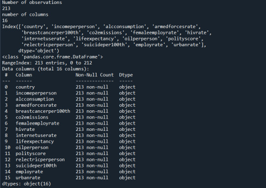
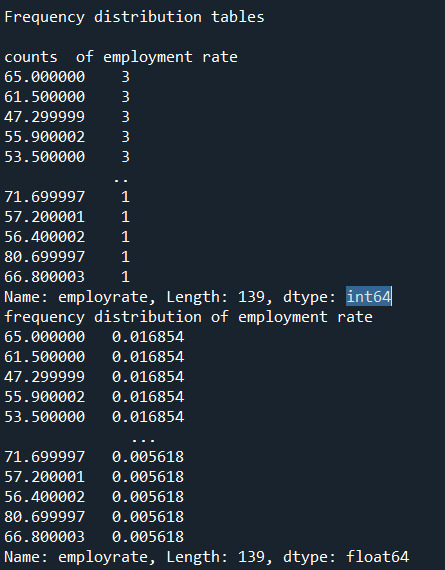
3) a few sentences describing your frequency distributions in terms of the values the variables take, how often they take them, the presence of missing data, etc.

Summary:

I added additional Pandas functions to help visualize the data below.

There was no need to subset the data since it's already aggregated per country. The 3 chosen variables span 213 countries and I would like to include each country in my study.

Typically, I would drop the blank cells from my percent calculations below, however the Python code we were presented with this week had "dropna=false".

Each of the 3 chosen GapMinder columns\variables has missing data. Removing the missing data from each column may not affect the overall research questions, however the same rows have different missing data, thus in aggregate removing all rows with missing values will likely have an impact on the research questions.

Rather than remove the rows with missing data another approach is to calculate the column mean and add it to the missing cells.

Variable Details:

Employ Rate:

"Employment rate" shows the number of times a particular Employment rate occurred. For example, a employe rate of 52.8 occurred 2 times in the data set.  

"Employe rate" is the number of times a particular employe rate occurred divided by the count of all employe rates, There are 213 countries\rows which also include blank cells.

Urban Rate:

Urban rate shows the rate of people living in urban areas. There are missing data in some countries. There are 2 countries with the maximum rate of 100 in the dataset.

"Urban Rate" is the number of times at which population of urban areas occurred divided by the count of all the urban rates. There are 213 countries in the whole dataset.

Oil per person:

"oilperperson" refers to the oil consumption per person on yearly basis. There are a lot of blank cells in the gapminder dataset. 70% percent of the countries oil per person consumption lies between 0-2. In the countries with high urban rate their seems to be more oil consumption per person.