#binormal vector

[johngreen-parody]

When your inner math major comes out of hibernation

[machudson]

Ok so if I'm understanding this right (this is just me parsing the topic & what's on the page, I assume you already know these things), this is about the Frenet-Serret frame, T(s) is a tangent vector, N(s) is the normal vector (derivative of T(s) with respect to s), and B(s) is the binormal vector = the cross product of those two. & theyre all unit vectors corresponding to a parametric curve in threespace. & this is something about curvature and torsion.

I'm getting that what's confusing you is related to B'(s) ?? I assume that the equation B'(s) = T'(s)×N(s) + T(s)×N'(s) comes from the product rule. I see you noted that T'(s) ~ N(s) and so their cross product = 0. Which simplifies it down to B'(s) = T(s)×N'(s). As this is a cross product with T(s) as one factor (are they called factors with cross products?? I forget), the end result B'(s) is perpendicular to T(s). hence the B'(s)•T(s) = 0 below. B'(s) is also perpendicular to N'(s) for the exact same reasons.

Wait I just noticed that this last circled bit with B'(s) has B'(s) on both sides of the equation... Yeah okay hmmm. Wait. Is this implying that B'(s) is a scalar multiple of N(s) ... Consulting wikipedia

GREAT. and you wrote below that 𝜏(s) = -B'(s)•N(s) so that all lines up. The question is how the hell did we get there.

Ohhh I think i may be understanding how we got here. There's the above bit that says B'(s)•B(s) = 0 meaning B'(s) and B(s) are perpendicular. So B'(s) is perpendicular to both B(s) and T(s), and N(s) is perpendicular to both B(s) and T(s), and there's probably a leap in logic I'm making here because I don't remember any formal theorems or definitions about a perpendicular basis of R3 or anything but I trust that it works, and so B'(s) is a scalar multiple of N(s). And I think 𝜏(s) gets defined from that. I THINK.

does anyone here understand fucking geometryyyyy i need help badly

[lawsofemotion]

Finished Chapter 11: Vector Functions and Curves!

[fulltestbank]

Test Bank For Calculus: Multivariable, 12th Edition Howard Anton

TABLE OF CONTENTS   PREFACE ix   SUPPLEMENTS x   ACKNOWLEDGMENTS xi   THE ROOTS OF CALCULUS xv   11 Three-Dimensional Space; Vector 657   11.1 Rectangular Coordinates in 3-Space; Spheres; Cylindrical Surfaces 657   11.2 Vectors 663   11.3 Dot Product; Projections 673   11.4 Cross Product 682   11.5 Parametric Equations of Lines 692   11.6 Planes in 3-Space 698   11.7 Quadric Surfaces 705   11.8 Cylindrical and Spherical Coordinates 715   12 Vector-Valued Functions 723   12.1 Introduction to Vector-Valued Functions 723   12.2 Calculus of Vector-Valued Functions 729   12.3 Change of Parameter; Arc Length 738   12.4 Unit Tangent, Normal, and Binormal Vectors 746   12.5 Curvature 751   12.6 Motion Along a Curve 759   12.7 Kepler's Laws of Planetary Motion 771   13 Partial Derivatives 781   13.1 Functions of Two or More Variables 781   13.2 Limits and Continuity 791   13.3 Partial Derivatives 800   13.4 Differentiability, Differentials, and Local Linearity 812   13.5 The Chain Rule 820   13.6 Directional Derivatives and Gradients 830   13.7 Tangent Planes and Normal Vectors 840   13.8 Maxima and Minima of Functions of Two Variables 845   13.9 Lagrange Multipliers 856   14 Multiple Integrals 866   14.1 Double Integrals 866   14.2 Double Integrals Over Nonrectangular Regions 873   14.3 Double Integrals in Polar Coordinates 882   14.4 Surface Area; Parametric Surfaces 889   14.5 Triple Integrals 902   14.6 Triple Integrals in Cylindrical and Spherical Coordinates 909   14.7 Change of Variables in Multiple Integrals; Jacobians 918   14.8 Centers of Gravity Using Multiple Integrals 930   15 Topics in Vector Calculus 942   15.1 Vector Fields 942   15.2 Line Integrals 951   15.3 Independence of Path; Conservative Vector Fields 966   15.4 Green's Theorem 976   15.5 Surface Integrals 983   15.6 Applications of Surface Integrals; Flux 990   15.7 The Divergence Theorem 999   15.8 Stokes' Theorem 1008   A Appendices   A Trigonometry Review (Summary) App-1   B Functions (Summary) App-8   C New Functions From Old (Summary) App-11   D Families of Functions (Summary) App-16   E Inverse Functions (Summary) App-23   READY REFERENCE RR-1   ANSWERS TO ODD-NUMBERED EXERCISES Ans-1   INDEX Ind-1   Web Appendices (online only)   Available in WileyPLUS   A Trigonometry Review   B Functions   C New Functions From Old   D Families of Functions   E Inverse Functions   F Real Numbers, Intervals, and Inequalities   G Absolute Value   H Coordinate Planes, Lines, and Linear Functions   I Distance, Circles, and Quadratic Equations   J Solving Polynomial Equations   K Graphing Functions Using Calculators and Computer Algebra Systems   L Selected Proofs   M Early Parametric Equations Option   N Mathematical Models   O The Discriminant   P Second-Order Linear Homogeneous Differential Equations   Chapter Web Projects: Expanding the Calculus Horizon (online only)   Available in WileyPLUS   Blammo the Human Cannonball -- Chapter 12   Hurricane Modeling -- Chapter 15         Read the full article

[quizllc]

A homomorphism sends a zero vector to the vector.

A homomorphism sends a zero vector to the vector.

A. Normal B. Binormal C. Zero D. Both A & B

[cgregorip5]

Intro p5 Sketch

Intro Sketch: https://editor.p5js.org/cgregori/full/HK_u7OEwo

I really like how easy it is to incorporate movement in p5, so I wanted this sketch to be able to move. I saw some Coding Train videos over break, and loved how accessible and understandable these videos were. The particle systems and flocking videos stood out to me. 

For this sketch, I saw The Coding Train’s acceleration vector video right after my Linear Algebra lecture, and I went from there. I took his mover code, and added a couple things to it, predominately random color and a wall collision checker. I also added an ability to add more movers to the canvas whenever a mouse is clicked.

I’ve had practice working with 2D coordinates before, so I wanted to push my boundaries and work with vectors. I like the somewhat-erratic way the orbs move on the screen, and I’m glad that the wall collision works mostly well.

This is less a self-portrait and more of an idea of the things I’m interested in. Maybe a self-interest-portrait?

Some future stuff that would be cool to add would be a way for an orb to check if it collides with another orb, and have the velocity vector change accordingly. That’s more complicated, but I’ve seen some stuff floating around on the internet on how to accomplish that goal. I also want to play around more with vectors, and eventually get into 3D vector space with normal vectors, binormal vectors and all that.

[multivarblogs]

Chapter 13 ~ Vector Functions

 Reflection

I think the hardest part of this chapter was remembering all the equations and when to use what. However, as I began to get a better grasp of what exactly things like a unit tangent vector were, I was able to better remember the when I understood how they worked. I’m proud that I was able to eventually find normal and binormal vectors without thinking twice. I think this finally clicked when I realized that T, N, and B all built off of each other because that helped me remember how to find them and what exactly they meant. I was also able to achieve my goal of getting above a 90% on the Webassigns.

Problems

In finding the curve of intersection, I solved for x and then substituted it into the equation for the cylinder. Vector valued functions were a main part of this unit and this problem helps emphasize the idea of splitting up the function into the x, y and z components. 

The curvature (K) is a measurement of how fast a curve is changing direction at a given point and I found it using the equation above. It can also be found by dividing the magnitude of the derivative of T(t) by the magnitude of the derivative of r(t).

An normal plane is a plane perpendicular to T(t) and an osculating plane is a plane perpendicular to B(t) so to find them I first had to find each of their equations and plug in the t value that does through the points.

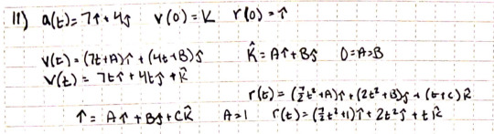
a(t) = v’(t) = r’’(t) so to find v(t) and r(t) you need to take the antiderivative of a(t) and v(t), respectively. It is important to remember to add the initial velocity/position when you take the antiderivative.

Goal

My goal for this unit is to not get more than two problems wrong on the Webassigns.

[realtalk-tj]

I'm interested in knowing the topics covered in Multivariable Calculus. Would you be able to point me in the direction of a curriculum or something similar?

Response from Flitwick: 

The school follows Stewart’s Multivariable Calculus, 4th edition for chapters 13-17. Here’s a brief outline of what you can expect to see (off the top of my head)

note: chapter titles are my own because I don’t remember what they are :P

Ch. 13, Three-Dimensional Geometry (and stuff): Quadric surfaces (like conics but in three dimensions), parameterizations and equations of points, lines, and planes, distances, vectors review

Ch. 14, Vector-Valued Functions and Light Differential Geometry: Doing BC Calc stuff (differentiation, integration) with vector-valued functions, arc-length parameterization, Frenet-Serret formulae (tangent, normal, binormal vectors; curvature, torsion), velocity and acceleration

Ch. 15, Functions of Multiple Variables: Limits of functions of multiple variables, differentiating functions of multiple variables, contour plots, manipulating and calculating partial derivatives (possibly when a function of multiple variables is held constant), directional derivatives, the gradient operator, extrema/critical points of functions of multiple variables, the method of Lagrange multipliers

Ch. 16, Integration Hell: Iterated integration, double/triple integrals over domains (in Cartesian, polar/cylindrical, spherical coordinates), Jacobian change of variables, simplifying calculations of integrals with symmetry considerations/other tricks

Ch. 17, Vector Fields and the Various Fundamental Theorems(TM) of Multivariable Calculus: Vector fields (and drawing them), arc-length integrals and line integrals for vector fields, path-independence/conservativity of vector fields and the Fundamental Theorem of Line Integrals, potential functions, the curl and divergence operators, Green’s Theorem, Stokes’ Theorem, determining whether a vector field is solenoidal, Divergence Theorem

Paul’s Online Math Notes are a great resource for multivariable calculus (stuff for this is listed under Calculus III) if you’re interested in looking at some of these topics.

[file-formats-programming]

Create Animated Scene, Create Primitive 3D Shapes & Convert Meshes to Binary Format using Java

What’s new in this release?

Aspose is proud to expand its components family with the addition of a new product known as Aspose.3D for Java 18.5. Aspose.3D for Java API has incorporated import and export features, and developers would be able to convert their 3D models to any supported 3D formats. All readable and writable supported file formats are listed in the documentation help topics "Read 3D document" and |Save 3D document" on blog announcements page. Aspose.3D for Java API includes support of creating 3D scene from scratch, defining Metadata of the 3D scene, creating primitive 3D Shapes and visiting sub nodes to convert meshes to custom binary format. With Aspose.3D for Java API, developers can generate and store tangent and binormal data for all meshes. The tangent and bitangent are orthogonal vectors with the Normal, and instruct about the rate of change of the texture coordinates over the mesh surface. Developers can also triangulate mesh, split mesh, convert primitive shapes to meshes, encode 3D mesh in the Google Draco file, convert all Polygons to triangles and generate normal data for all meshes of 3D scene. Aspose.3D for Java API supports rendering the animated scene, and the help topic narrates prerequisites to move an object. Developers can also set up the Camera with a target to constrain. Aspose.3D for Java API supports rotating objects in a 3D scene, add node hierarchy, share geometry data of mesh between multiple nodes, concatenate Quaternions apply to 3D objects, define Mesh from scratch, set up normals or UV on objects and also add Material.  This release includes plenty of new features as listed below

Define Metadata, create Primitive 3D Shapes and convert Meshes to binary format

Add Asset Information to 3D document

Create Scene with Primitive 3D Shapes

Save 3D Meshes in Custom Binary Format

Manipulate Objects in 3D Scene

Create an Animated Scene

Work with Geometric data of 3D Scene

Generate Normal Data for All Meshes of 3D Model

Convert all Polygons to triangles in 3D Model

Newly added documentation pages and articles

Some new tips and articles have now been added into Aspose.3D for Java documentation that may guide users briefly how to use Aspose.3D for performing different tasks like the followings.

Save 3D Document

Read 3D document

Overview: Aspose.3D for Java

Aspose.3D for Java is a feature-rich Gameware and Computer-Aided-Designing (CAD) API that empowers Java applications to connect with 3D document formats without requiring any 3D modeling software being installed on the server. It supports most of the popular 3D file formats, allowing developers to easily create, read, convert & modify 3D files. It helps developers in building mesh of various 3D geometric shapes; define control points and polygons in the simplest way to create 3D meshes.  It empowers programmers to easily generate 3D scenes from scratch without needing to install any 3D modeling software.

More about Aspose.OCR for Java

Homepage of Aspose.3D for Java

Download Aspose.3D for Java

Online documentation of Aspose.3D for Java

[brianfreemann-blog]

Learning About Shaders(Vertex Shader)

A vertex shader is executed for each vertex that is submitted by the application, and is primarily responsible for transforming the vertex from object space to view space, generating texture coordinates, and calculating lighting coefficients such as the vertex's tangent, binormal and normal vectors.

[programming-languages-en-blog]

High-Level Shading Language

A scene containing several different 2D HLSL shaders. The statue is distorted purely physically, while the inner door texture is physically distorted based on color intensity. The square in back is transformed and rotated via a shader, and the water reflection and partial transparency at the bottom have been added by a final shader acting on the entire scene. The High-Level Shader Language or High-Level Shading Language (HLSL) is a proprietary shading language developed by Microsoft for the Direct3D 9 API to augment the shader assembly language, and went on to become the required shading language for the unified shader model of Direct3D 10 and higher. HLSL is analogous to the GLSL shading language used with the OpenGL standard. It is very similar to the Nvidia Cg shading language, as it was developed alongside it. HLSL shaders can enable profound speed and detail increases as well as many special effects in both 2d and 3d computer graphics. HLSL programs come in five forms: pixel shaders (fragment in GLSL), vertex shaders, geometry shaders, compute shaders and tessellation shaders (Hull and Domain shaders). A vertex shader is executed for each vertex that is submitted by the application, and is primarily responsible for transforming the vertex from object space to view space, generating texture coordinates, and calculating lighting coefficients such as the vertex's tangent, binormal and normal vectors. When a group of vertices (normally 3, to form a triangle) come through the vertex shader, their output position is interpolated to form pixels within its area; this process is known as rasterisation. Each of these pixels comes through the pixel shader, whereby the resultant screen colour is calculated. Optionally, an application using a Direct3D 10/11/12 interface and Direct3D 10/11/12 hardware may also specify a geometry shader. This shader takes as its input some vertices of a primitive (triangle/line/point) and uses this data to generate/degenerate (or tessellate) additional primitives or to change the type of primitives, which are each then sent to the rasterizer. D3D11.3 and D3D12 introduced Shader Model 5.1. More details Android, Windows

[maryssnotes]

[arxt1]

A novel approach for the analysis of the geometry involved in determining light curves of pulsars. (arXiv:1909.09583v1 [astro-ph.HE])

In this work, we introduce the use of the differential geometry Frenet-Serret equations to describe a magnetic line in a pulsar magnetosphere. These equations, which need to be solved numerically, fix the magnetic line in terms of their tangent, normal, and binormal vectors at each position, given assumptions on the radius of curvature and torsion. Once the representation of the magnetic line is defined, we provide the relevant set of transformations between reference frames; the ultimate aim is to express the map of the emission directions in the star co-rotating frame. In this frame, an emission map can be directly read as a light curve seen by observers located at a certain fixed angle with respect to the rotational axis. We provide a detailed step-by-step numerical recipe to obtain the emission map for a given emission process, and give a set of simplified benchmark tests. Key to our approach is that it offers a setting to achieve an effective description of the system's geometry {\it together} with the radiation spectrum. This allows to compute multi-frequency light curves produced by a specific radiation process (and not just geometry) in the pulsar magnetosphere, and intimately relates with averaged observables such as the spectral energy distribution.

from astro-ph.HE updates on arXiv.org https://ift.tt/2LFOLfg