#countifs function

[techalertr]

COUNT Function all Variants in one Video | MS Excel Detailed video : https://youtu.be/DvrVhap1H0I Countifs function in ms excel : https://youtu.be/LWF-zoEIHP4 #techalert #shorts #excel #technical #howto #trending #viralvideo #instagram #trending

[ninjagobythenumbers]

Ninjago Species by the Season

I made this chart upon @weirdcatbean's request. I also wanted to include allignment and centrality on this chart, but as you can see that would get pretty busy.

Here's the percentages.

Interestingly, it keeps a pretty consistent human:non-human ratio. The earlier seasons actually have less humans percentage wise, which I did not expect. However, I should note that this chart includes every single named character, so while yes there may be 36 humans in Seabound for instance, 19 of them are ensemble who were just there for Nya's funeral. I'll be making an improved version of this chart later that's a bit easier to read and includes some more relavant data points. Now, you may be wondering, why didn't I include what the chart looks like without the inclusion of ensemble from the beginning. I admit, normally I would. To explain why I didn't, I have to tell the story of how I came up with these numbers.

Methodology

While I could have just tallied up individual species season by season, I knew I would probably want to play with the data in other ways besides just this one chart. Thus, I undertook the massive endeavor of indexxing every Ninjago character by Name, Type, Allignment, Species, Gender, and Season. For instance, here's the pilot season.

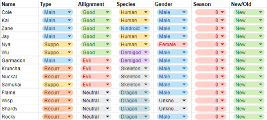
You may be wondering what the New/Old column is all about. In order to include the full character breakdown for each season, I had to make new entries of each character every season. This created a lot of repeats, so to separate unique characters from repeats I noted whether character's were introduced with this season (new) or whether they were a repeat (old). This was also useful in that it allowed me to alter the criteria of a character with each season so I can accomadate for changes such as Cole turning into a ghost. Once I had compiled this data (839 entries and 292 unique characters), I attempted to use Google Sheets' pre-provided data analysis.

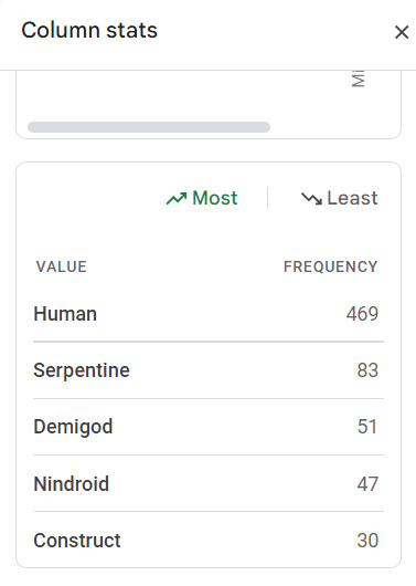
It was sort of useful, but it would only show the top 4 and bottom 4 frequencies and I couldn't copy and paste the data. It also was a bit fussy around filters. Thus, I did something a bit wonky where I filtered by season and just copy pasted the column into a different sheet.

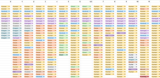
I then used functions (ex: =COUNTIF(AC3:AC1002, "Skeleton")) to create my raw data table which you can view above. This process worked but it had a lot of problems. It was time consuming, didn't allow me to employ multiple filters, and, most importantly of all, it wasn't allowing me to use this data I had spent days compiling to its full extent. Thus, I decided to create a sort of search engine for Ninjago characters.

This search engine allows me to input criteria and recieve not only the total characters that fit the criteria, but a list of all of their entries. The fact it lists all of their entries may not sound that impressive, but trust, it is. (For me at least) Here's an example search of good, recurring Serpentine.

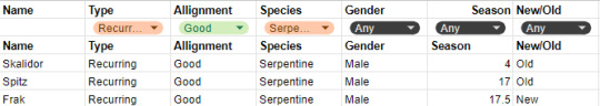
I am very excited about the potential of this tool. It's going to allow me to create a lot of great charts, including an improved Species by Season chart. For now though, I'm only uploading the original requested chart, because creating this tool has taken the better part of my day. I plan on sharing it, but I still need to work out a few kinks so you can look forward to that as well. I know I already said it, but I'm so, so excited about what I'll be able to make. Here's a preview to the search if you're interested. It also includes all my previous spreadsheets, but I'm still working out some formatting issues and stuff.

[onecooooooolcat]

a filter function nestled in a counta function is like if the countifs function actually served cunt

[stray-crow]

hi!! thought i'd direct my ask here since it's writing related -> how did you set up the google sheets to set and track word goals?? i opened up a sheets but it's a bit intimidating ;;

i'm guessing you do Insert>function>??? one of those? but idk which

there are a lot of different ways!! some basics to know:

the main functions i may use here are =SUM, =AVERAGE, =COUNTIF then follow the formula outline

more frequently i stick = in the formula box then select cells (or tab you want then its cells) with my mouse (a quicker way than typing cell or tab names)

but you can also limit cells usage by editing formulas directly in the cell you want to see the = in (like, you can have a cell with "=2+2" or a cell with "=A1+A2" with the numbers in them. both cells will have the same total calculated by the = but the formula bar will look different). Data Managers™️ recommend keep everything visible in cells, but we aint publishing this so do what you want

i also use cell formatting as % or date or whatever for less formula writing (% for example, i otherwise gotta do whatever math is needed for calculating that when i can just do the basics then ask it to do the rest AND it adds a % sign for me)

now let me go from least to most complicated set-up at start:

1. Total at Bottom

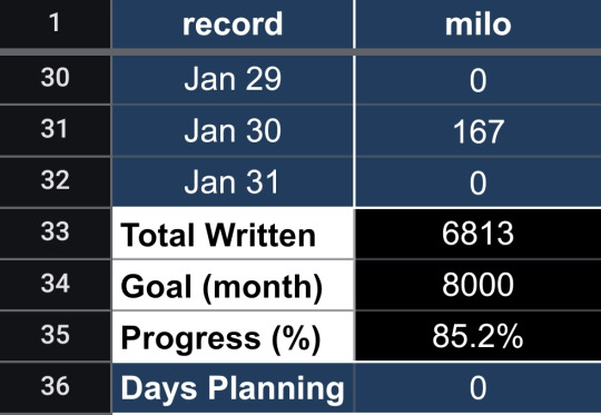
i got this settup to track multiple people at once, but you can keep the record column as Day 1, Day 2, etc and change the name columns to be months. Formulas:

row 33 Total Written =SUM(B2:B32) (alter the letter and number depending on column and days in month)

row 34 Goal (month) [free write #]

row 35 Progress (%) =B33/B34 , aka =[Total Written cell/Goal (month cell] format as %

row 36 Days Planning =COUNTIF(B2:B32, "planning") (or whatever specific word you want)

you can also have a year total somewhere, which you can see examples of how to in the last method

2. Weekly Goal

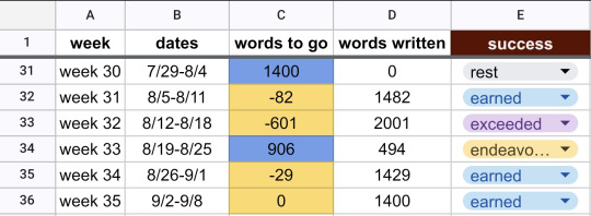
there's more manual in this so far which makes it easier to setup, harder to keep up on. columns week, dates, and words written are write-in (the last which i may =#+#+# throughout), but formulas:

column c words to go =1400-D31, aka =[word count goal]-[relevant "words written" cell]. conditional formatting (which i may swap the colors):

column e success is a drop-down menu which i forget how to create every time... look up "how to create drop-down menu in [spreadsheet program of choice]". i manually select the success based on vibes: earned, endeavored, exceeded, and resting

3. Detailed Year

there are two tabs here with more initial setup but less to manage later. they read from each other (what the ! does in a formula). starting with the daily data tab:

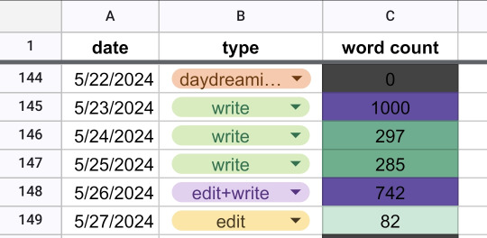
column date is formatted for calendar

column type is formatted with a drop-down menu, which the thought is to later make a pivot table counting the frequency of write, edit, edit+write, and daydreaming.

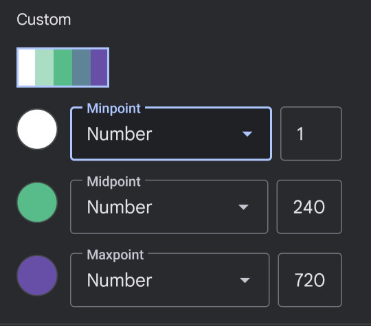
column word count is a manual input with conditional formatting

then the year tracking tab:

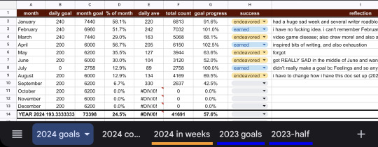
the free write-in columns are month, daily goal, and reflection. the column success is a drop-down i manually select at end. everything else has formulas:

column c month goal =[daily goal cell]*[# days of that month]

column d % of month will look like =(COUNTIF('2024 count'!C246:C275, ">0"))/30 , aka (COUNTIF('[name of daily data tab]'![relevant cell range from tab],">0"))/[days of month] formatted as %

column e daily ave is =AVERAGE(('[name of daily data tab]'![relevant cell range])

column f total count is =SUM('[name of daily data tab]'![relevant cell range]

column g goal progress is =[total count cell]/[month goal cell] formatted as %

the total row at the bottom goes like

daily goal =AVERAGE([above cells])

month goal =SUM([above cells])

% of month =AVERAGE([above cells])

daily ave =AVERAGE([above cells])

total count =SUM([above cells])

goal progress =AVERAGE([above cells])

yea that's about it

[ellisnyeland]

oh I am a GENIUS, countif function I am kissing you on the MOUTH

does anyone want a tutorial post on how to set up a NaNoWriMo stats page in LibreOffice Calc that has pretty much all the same functions of the one on their website? should be pretty easy to make it work in Excel or Google Sheets

[tparadox]

While I was able to use the holiday Monday at work to catch up on stuff I haven't been able to do in the last six weeks I've been doing my job alone, I spent way more of that time than I wanted to in trying to find a way around Excel breaking my labor saving spreadsheet by refusing to follow its own rules.

I help out my supervisor by turning the reports our phone system generates into a chart of call times she can analyze for coverage purposes. There are two hurdles the way it generates the reports creates. One of them is that the date, beginning time, and ending time, are all in the same cell of its line, and the other is that if there's no active call time in that span, it will more likely than not skip that span.

The easiest way I've come up with to find those times it skipped is to break up the time stamps into separate date, start, and stop cells, and then use conditional formatting to highlight the start times that are different from the end time of the line above. Originally I was using text to columns to do this, but then I decided I wanted to automate that. I set up a spreadsheet that would take the file name of the report and fetch the date and time cell from it, then an array of cells using the MID function to pull out the individual pieces of it.

It worked great! I could just tell it the file to look at and it got the data I needed. And then I'd go to add a line for a skipped time span and all of the formulas would break, because they were referenced based on the line number, and Excel ever so helpfully updates those references when your data moves. But it's okay because if you don't want the reference to be updated, there's a character for that. To keep the same line number, use B$2 instead of B2.

I worked out a fancy formula with INDIRECT, LEFT, and the new to me FORMULATEXT function to automatically assemble a new version of the formula with the crucial absolute reference for each row, since the absolute meant it wouldn't update by line if I just filled down and I was not going into over 300 cells to add one character by hand.

EXCEPT! Marking the reference as absolute only freezes the reference for pasting and directional filling! It turns out it totally ignores the $ if you're shifting and inserting! Excel broke my plans because it doesn't follow its own rules!

After like two hours of beating my head against it and reading a bunch of forum help threads where the answer was "just use INDIRECT" when I was already using INDIRECT, using COUNTIF to count only the cells above that had data in them seemed promising, but it kept giving reference errors as part of the INDIRECT, probably because the COUNTIF syntax needs you to tell it what to look for, and I think the quotation marks around the asterisk weren't playing nicely with the quotation marks of the INDIRECT even though I was using " for the latter and ' for the former. Finally I started looking into other COUNT_____ functions and it turns out that plan old COUNT does exactly what I was looking for. Where "count cells that have data" with COUNTIF needs you to specify cells containing "*", COUNT just does it. By some miracle, I found the right syntax to have the INDIRECT assemble the COUNT with a range from B1 to (current cell) in only one or two tries, and now I finally have a formula that doesn't care if I add lines which are empty in the column it's looking at.

Now I just need to automate adding the missing rows and filling in the zero values in the column I'm doing this all for, but that seems beyond what I can do with just Excel on its own. Seems like something that would be simple to execute in Python if I export a CSV, and if I could get anything to work in VBasic I could probably do a macro, but I'd prefer not to step it out of Excel and back in, and I don't think our workstations have Python, and if they don't have it, I can't add it...

[tccicomputercoaching]

Beyond Basics: Advanced Excel for Careers

When you think of Microsoft Excel, you might picture simple spreadsheets for organizing data or basic calculations. Yet, in almost all industries, Excel is far more than a mere table. It is data analysis, reporting, and automation tool. Going beyond the basics, becoming an advanced Excel pro leads to a career fast track, converting an ordinary data user to the master.

Companies across industries are drowning in data in today's data-driven world. They require workers who can handle data, extract insights, display information well, and automate processes. Advanced Excel skills thus make you an awesome asset in the finance firms, marketing agencies, HRs, and operations departments.

Why Advanced Excel Skills are Resisted in Career Growth

Many would consider basic Excel skills to be the only requirement of a job; however, the reality is that further potentials of Excel are increasingly sought after by employers. Here is why getting the hang of advanced Excel is crucial:

Data Analysis Prowess: You are able to analyze big sets of data instantaneously; identify trends; and come up with useful business decisions.

Report Creation: Develop fully interactive reports and dashboards that provide a visual representation of complex information to stakeholders.

Automation & Efficiency: Consider the fascination of automating repetitive tasks anymore and save human beings hours of work while few errors can occur due to manual operations.

Problem-Solving: Advanced functions can be used to model complex business problems, from financial decision-making to resource allocation.

Employability: Advanced Excel skills appear on almost every job listing and are sometimes considered the top requirement for many.

Key Advanced Excel Skills to Master

If you want to truly move beyond the basics, then consider sharpening your skills around these powerful features:

Pivot tables and Pivot charts: Learn to summarize, analyze, explore, and present large amounts of data interactively and flexibly. These are best used for quick reporting and spotting trends.

Advanced functions (VLOOKUP, HLOOKUP, INDEX, MATCH, IF, SUMIFS, COUNTIFS): Beyond simple sums, these allow complex lookups and conditional aggregations or tests over multiple criteria. INDEX and MATCH are a particularly powerful combo.

Data Validation: Do data cleansing by defining rules that restrict what can be entered in a cell, thus preventing errors and promoting inconsistency.

Conditional Formatting: Highlight data based on given criteria; this will help trends, exceptions, and anomalies stand out at a glance.

What-If Analysis (Goal Seek, Scenario Manager, Data Tables): Play with perhaps various scenarios and make predictions for expected results once variables have been changed; this is very important for planning and decision-making.

Macros & VBA (Visual Basic for Applications): Record or write custom code, relying heavily on automation to eliminate tedious manual tasks, create custom functions, and develop very powerful user interfaces within the Excel environment itself-this is an efficiency game-changer.

Power Query & Power Pivot: These built-in tools allow for advanced cleansing and transformations and creation of sophisticated data models, working with a much bigger volume of data compared to a traditional Excel file.

Career Roles Where Advanced Excel Shines

Having those skills opens countless career openings:

Financial Analyst: This is important for financial modeling, budgeting, forecasting, and investment analysis.

Business Analyst: For market research, performance measurement, and strategic planning.

Data Analyst: For cleaning, analyzing, and making data easier to understand from various sources.

Project Manager: For progress tracking, resource management, and detailed scheduling.

Marketing Analyst: Measuring campaign performances, analyzing customer data, and trends in sales.

Operations Manager: For workflow optimization, inventory handling, and logistics conversation.

Your Road to Advanced Excel Mastery

If you aspire to level up, taking an Advanced Excel course or a Data Analytics course in Ahmedabad is strongly recommended. These programs dive deep into advanced functions, tools, and best practices, typically going further with actual project executions to churn out a mature portfolio. For a student seeding for their first job or a working professional looking to rank higher, investing in advanced Excel skills will pay dividends through their entire career. Become the Excel expert your workplace needs. At that stage, your livelihood will be fostered by your flourish!

Contact us

Call now on +91 9825618292

Visit Our Website: http://tccicomputercoaching.com/

[advancedexcelinstitute]

How to Handle Duplicates in Excel Without Losing Important Data

If you’ve ever worked with large Excel sheets, you know how easily duplicate entries can sneak in. From client databases to inventory records, these repeated values can distort your analysis and lead to reporting errors. The key isn’t just removing them — it’s doing so without deleting valuable information.

Many people jump straight to the “Remove Duplicates” button in Excel, which can work well, but only if you’re sure of what you’re deleting. Without a careful review, you might end up losing original data that shouldn’t have been removed.

A smarter way is to use Excel’s built-in features more strategically. For instance, Conditional Formatting lets you highlight duplicates visually before taking any action. This gives you time to scan through the data and verify what’s truly redundant.

Another helpful method is to use Excel’s Advanced Filter. This allows you to copy only unique values to another location, keeping your original data intact. It’s especially useful when you want to create a clean version of your data for analysis without changing the source file.

Formulas also come in handy. By using functions like COUNTIF, you can flag rows that appear more than once. You can then decide manually which entries to keep or discard, giving you full control over your data.

Whatever method you choose, the golden rule is this: always back up your file before making changes. That way, even if something goes wrong, you can recover the original without stress.

Removing duplicates in Excel doesn’t have to be risky or complicated. With a few smart techniques, you can keep your data clean and organized while protecting valuable information. Whether you’re a beginner or an experienced Excel user, learning the right approach will help you work more efficiently and avoid costly mistakes.

For a step-by-step walkthrough on these methods — including tips, examples, and best practices — check out the full article. It’s a great resource if you want to master Excel’s data-cleaning features without compromising your data.

[rohitdigital1001]

Advanced Excel Courses at DICS Innovatives

In today's data-driven world, Excel skills are essential for professionals across various industries. If you're looking to enhance your Excel capabilities, enrolling in an advanced Excel institute in Pitampura can make a significant difference. For residents of Pitampura, one of the best advanced Excel institutes is DICS Innovatives.

Key Features of Advanced Excel

Data Analysis and Reporting

Advanced Excel empowers you to perform in-depth data analysis and generate comprehensive reports. With tools like:

Power Query: Transform and clean your data efficiently.

Power Pivot: Create sophisticated data models and perform complex calculations across multiple tables.

Automation with Macros and VBA

For repetitive tasks, mastering Macros and VBA (Visual Basic for Applications) can save time and reduce errors. You’ll learn how to:

Record and edit Macros to automate routine processes.

Write custom VBA scripts to extend Excel's capabilities, allowing for tailored solutions to specific problems.

Data Visualization Techniques

Understanding how to represent data visually is crucial for effective communication. At DICS Innovatives, you'll learn to:

Create advanced charts, including waterfall, funnel, and radar charts.

Use conditional formatting to highlight key data points and trends, making reports more intuitive.

Scenario Analysis and Forecasting

Excel is a powerful tool for financial modeling and forecasting. You’ll explore:

What-If Analysis: Use tools like Goal Seek and Data Tables to analyze different scenarios.

Forecasting: Learn techniques to predict future trends based on historical data, utilizing Excel’s built-in forecasting tools.

Why Choose DICS Innovatives?

DICS Innovatives stands out as a premier institute for advanced Excel training. Here are some reasons why you should consider their courses:

1. Comprehensive Curriculum

DICS Innovatives offers a well-structured curriculum that covers all aspects of advanced Excel. Key topics include:

Advanced Formulas: Learn to use complex functions such as SUMIFS, COUNTIFS, and array formulas to perform sophisticated calculations.

Pivot Tables and Charts: Master the art of summarizing large datasets quickly and effectively, creating dynamic reports that help in decision-making.

Data Validation: Implement data validation rules to maintain data integrity and ensure accurate data entry.

2. Experienced Instructors

The instructors at DICS Innovatives are industry experts with extensive experience in using Excel for real-world applications. Their practical insights help students understand the nuances of Excel and its applications in various business scenarios.

3. Flexible Learning Options

DICS Innovatives offers flexible learning options, including weekend batches and online classes, making it convenient for working professionals to enhance their skills without disrupting their schedules.

4. Certification

Upon completion of the course, participants receive a certification that adds value to their resumes and demonstrates their proficiency in advanced Excel skills—an asset in today’s job market.

Conclusion

If you're searching for the best advanced Excel institute in Pitampura, look no further than DICS Innovatives. Their comprehensive courses, expert instructors, and practical training methods will equip you with the skills needed to excel in your career. Don’t miss the opportunity to enhance your Excel proficiency and open up new avenues in your professional journey!

[technologytrendsinit]

Mastering Excel: Unlocking the Power of Advanced Formulas

In the world of data analysis and management, Microsoft Excel has long been a trusted companion for professionals across various industries. While the software’s basic functionality is well-known, many users often overlook the true power that lies within its advanced formulas. In this blog post, we’ll dive deep into the realm of Excel’s advanced formulas, exploring how they can streamline your workflow, enhance your data analysis, and unlock new levels of productivity.

Understanding the Basics of Excel Formulas At the core of Excel’s functionality are its formulas, which allow users to perform a wide range of calculations and manipulations on their data. The standard formulas, such as SUM, AVERAGE, and COUNT, are well-known and widely used. However, Excel’s advanced formulas take things to the next level, providing more sophisticated and customizable solutions to complex problems.

The Power of Excel’s Advanced Formulas Excel’s advanced formulas are like a toolbox filled with specialized tools, each designed to tackle specific data-related challenges. These formulas offer a level of complexity and flexibility that can significantly enhance your analytical capabilities. Let’s explore some of the most powerful advanced formulas and how they can benefit your work:

VLOOKUP: This formula is a game-changer when it comes to cross-referencing data across different tables or worksheets. By using the VLOOKUP function, you can quickly find and retrieve corresponding values, making it a valuable tool for data consolidation and reporting.

SUMIFS and COUNTIFS: These advanced formulas allow you to perform complex conditional summations and counts, respectively. They enable you to aggregate data based on multiple criteria, providing a more targeted and insightful analysis.

INDEX and MATCH: The combination of these two formulas is a powerful way to look up and retrieve data from a range of cells, even if the data is not organized in a traditional table format. This is particularly useful when dealing with dynamic or non-standardized data sources.

PIVOT TABLES: While not a formula per se, pivot tables are an advanced feature in Excel that allows you to quickly analyze and summarize large datasets. By organizing and aggregating data in a flexible manner, pivot tables enable you to uncover insights and trends that may not be readily apparent in the raw data.

ARRAY FORMULAS: Array formulas are a unique and powerful type of formula that can perform operations on entire arrays of data, rather than individual cells. They are particularly useful for complex calculations, data manipulation, and statistical analysis.

OFFSET and INDIRECT: These advanced formulas provide dynamic and flexible ways to reference and manipulate cell ranges, making them valuable for tasks such as creating interactive dashboards, automating reports, and building complex financial models.

LOOKUP and CHOOSE: The LOOKUP formula allows you to search for a value in a range and return a corresponding value, while the CHOOSE formula lets you select a value from a list based on an index number. These formulas can be particularly useful for data lookup and decision-making processes.

Mastering Advanced Formulas: Practical Applications Now that you’ve been introduced to some of the most powerful advanced formulas in Excel, let’s explore how you can apply them to real-world scenarios:

Financial Analysis: Advanced formulas can be invaluable in financial modeling and forecasting. For example, you can use SUMIFS to calculate total revenue or expenses based on multiple criteria, such as product category, region, or time period.

Sales Reporting: Combine VLOOKUP and SUMIFS to create comprehensive sales reports that consolidate data from multiple sources, allowing you to analyze performance, identify trends, and make informed decisions.

Inventory Management: Use advanced formulas to track and manage your inventory, automating calculations for reorder points, stock levels, and more. This can help you optimize your supply chain and minimize the risk of stockouts or overstocking.

HR and Payroll: Advanced formulas can streamline HR and payroll processes, such as calculating overtime pay, deductions, and employee benefits. SUMIFS and COUNTIFS can be particularly useful in these scenarios.

Data Validation: Leverage advanced formulas to implement data validation rules, ensuring the integrity and accuracy of your data. This can include checks for duplicate entries, data range validation, and more.

Project Management: Utilize advanced formulas to track project timelines, budgets, and resource allocation. Formulas like DATEDIF and NETWORKDAYS can help you monitor progress and identify potential bottlenecks.

Marketing Analytics: Advanced formulas can be used to analyze marketing data, such as campaign performance, lead generation, and customer retention. Formulas like CONCATENATE and TRIM can help you clean and prepare data for analysis.

Mastering the Art of Advanced Formulas Becoming proficient in Excel’s advanced formulas requires a combination of practice, patience, and a willingness to explore. Start by familiarizing yourself with the basic syntax and structure of each formula, then experiment with different use cases to understand their full potential. Many online resources, such as tutorial videos and Excel forums, can be invaluable in your learning journey.

As you become more comfortable with advanced formulas, consider creating your own custom formulas or combining multiple functions to tackle complex problems. Embrace the creative aspect of Excel and challenge yourself to find innovative solutions that streamline your workflow and enhance your data analysis capabilities.

Conclusion: Excel’s advanced formulas are the keys to unlocking the true power of the software. By mastering these specialized tools, you can transform your data analysis, reporting, and decision-making processes, ultimately leading to increased productivity, better-informed decisions, and a more efficient work environment. Take the time to explore and experiment with Excel’s advanced formulas, and you’ll soon discover a world of new possibilities at your fingertips.

[fromdevcom]

There are hundreds of built-in functions in Microsoft Excel. Furthermore, you can use these functions together in different combinations to create powerful formulas. The ability to create formulas in Excel that solve complex problems is largely what makes the application so legendary. With that in mind, we will now look at 10 Excel functions that you should add to your repertoire. IFERROR The IF function is probably one of the most widely used functions among Excel pros. It is a logical function; if something is true then do something, otherwise do something else. The ‘IF’ function allows you to build metadata - a set of data used to describe other data. Those same pros that use ‘IF’ also use the ‘IFERROR’ function to handle errors in their formulas. We can use ‘IFERROR’ to specify an alternative value where a calculation might result in an error. Let’s look at the ‘IFERROR’ function’s syntax:                       =IFERROR(value, value-if-error) There are two arguments in this formula: ‘value’ and ‘value-if-error’. The ‘value’ argument is the parameter the function tests for an error. This is most often another formula itself. Then the ‘value-if-error’ argument is the replacement value the user has selected for ‘IFERROR’ to return if the ‘value’ parameter does result in an effort. The ‘value-if-error’ can be an actual static value such as a string or a number, but it can also itself be another formula. In the example that follows, we have an average price calculation in the ‘Average Price’ column. It is a simple division calculation that is susceptible to a divide by zero error (#DIV/0!). In cell D6, this is precisely what has happened. However, by using the ‘IFERROR’ function, we can ensure that the value ‘0’ gets returned to the cell in the case of an error. Note the improvement to our result for row 6 in cell E6. COUNTIF Another popular ‘IF’ based function is ‘COUNTIF’. This function counts cells in a range where some specified condition is met. The syntax is simple. There are two arguments: ‘range’ and ‘criteria’. The ‘range’ argument is the range in which you are searching for the ‘criteria’. The ‘criteria’ argument is the specific condition that needs to be met for the count                                  =COUNTIF(range, criteria) In the following example, we use ‘COUNTIF’ to count the number of employees by their years of service. Our ‘range’ argument is the column containing the ‘Year of Service’ for each employee, or “D2: D19” (the dollar signs preceding the column and row references are simply there to ‘lock’ the range for dragging the formula to other cells). The ‘criteria’ argument is the years of service (1, 2 or 3). We could have placed the literal number values for ‘Years of Service’ as our ‘criteria’, but in this case, we opted to use the cell references for each (“F3”, “F4”, and “F5”, respectively). The ‘COUNTIF’ formula in each returns the count of employees corresponding to each value in ‘Years of Service’ in column G. Note the formulas for each row in column H. CONCATENATE The ‘CONCATENATE’ function is one of the most widely used in Excel. A point worth noting is that Microsoft introduced two new functions in Excel 2016 that will eventually replace ‘CONCATENATE’. They are ‘CONCAT’, a more flexible version of its predecessor, and ‘TEXTJOIN’. However, since not all Excel users have upgraded to Excel 2016, we will look at ‘CONCATENATE’. The ‘CONCATENATE’ function combines strings of text and/or numerical values. Syntactically, this simply means placing the values you want to concatenate in sequential order, separated by commas. You can use either literal values or cell references as your arguments. You can use a combination of both as well.                                         =CONCATENATE(text1,[text2],…) In the following example, we have two separate lists: first names and last names. Using the ‘CONCATENATE’ function, we will combine them in a column where we have the last name, then the first name separated by a comma.

Then we can sort each by the last name in alphabetical order. VLOOKUP If you have spent much time with anyone with a reasonable amount of proficiency using Excel, you have likely heard of ‘VLOOKUP’. Like its sibling, ‘HLOOKUP’, it will search a table of values based on a criteria value. The ‘VLOOKUP’ function will search the first column of a table for a criteria value and return a value from some specified number of columns to the right of that first column. The function consists of four arguments.                  =VLOOKUP(lookup_value, table_array, col_index_number, [range_lookup]) The first argument is the ‘lookup_value’ is the value ‘VLOOKUP’ seeks a match for in the ‘table_array’ argument. In the following example, this is the cell reference ‘E2’ where we see the string ‘Finance’. We could have just as easily used the literal string ‘Finance’ as our ‘lookup_value’ argument. But using the cell reference allows us to change the value in ‘E2’ without changing the formula. The ‘table_array’ is the table of values ‘VLOOKUP’ will seek a match for ‘Finance’ in the first column. Since our table is ‘A2: C7’, the match for our ‘lookup_value’ is on the first row (cell ‘A2’) of our ‘table_array’, The ‘col_index_number’ argument is the number of the column from which we want ‘VLOOKUP’ to return a match on the same row from the ‘lookup_value’. In our case, we want ‘Average Years of Service’ in our formula in cell ‘F2’. This means we will insert ‘2’ as our ‘col_index_number’ argument since ‘Average Years of Service’ is the second column in our ‘table_array’. The ‘range_lookup’ argument is an optional argument as denoted by the square brackets. This argument can be one of two values: TRUE or FALSE. A TRUE value tells the ‘VLOOKUP’ to return an approximate match while a FALSE value tells it to return an exact match. When omitted, the default for the formula is an approximate match. In the following example, we can easily look up the average years of service and the average salary for employees by specifying the department. An insider trick regarding ‘range_lookup’: try using ‘1’ and ‘0’ as a substitute for TRUE and FALSE, respectively. This is a shortcut that works just the same. Note in ‘G2’ our ‘VLOOKUP’ uses ‘0’ instead of FALSE. INDEX And MATCH The combination of ‘INDEX’ and ‘MATCH’ function gives users the ability to retrieve data from a table by specifying the row and column condition. Combining the two in a single formula creates one of the most well-known lookup formulas used. The most basic example of what the ‘INDEX’ function does is that it takes an array, like a column of names. Then it takes a second argument, ‘row_num’, and returns the value from the array on that row.                                       =INDEX(array, row_num, [column_num]) Note that since we are working with a single column, we omit the optional ‘column_num’ argument since it is implied. However, if we were working with an array that had more than one column, we would use the ‘column_num’ argument in the same way we use the ‘row_num’ argument. ‘INDEX’ will return the value at the intersection of the two in the specified ‘array’. In the following example, the ‘column_num’ is understood to be 1. This means the formula finds the value at the intersection of row 6 and column 1 of our ‘array’, ‘A2: A19’. The ‘MATCH’ function takes a ‘lookup_value’, a ‘lookup_array’, and an optional ‘match_type’ argument. The ‘match_type’ argument allows for one of three values; ‘-1’ for less than, ‘0’ for an exact match, or ‘1’ for greater than.                      =MATCH(lookup_value, lookup_array, [match_type]) In the next example, we pass in a string value for the ‘lookup_value’ and ‘0’ to ‘match_type’ for an exact match. See cell ‘C12’ for the result. Now you have seen how you can find the row on which a value exists in a column using the ‘MATCH’ function. You have also seen how you can find the value in a cell by passing in a row number to the ‘INDEX’ function.

Imagine you had a second column with email addresses that you wanted to look up by employee name. See if you can figure out how to combine ‘INDEX’ with ‘MATCH’ to do just that. Hint: substitute the ‘MATCH’ formula for the ‘row_num’ argument in the ‘INDEX’ formula – then make sure you select the email column as the ‘array’ for your ‘INDEX’ function. GETPIVOTDATA If you have ever tried referring to a cell or range in a Pivot Table, you have probably seen ‘GETPIVOTDATA’. The GETPIVOTDATA function helps retrieve data from a pivot table using the corresponding row and column value. This function is yet another type of lookup function but for Pivot Table users. It provides a direct method of retrieving tabulated data from Pivot Tables.                  =GETPIVOTDATA(data_field ,pivot_table, [field1, item1], …) The first argument, ‘data_field’, refers to the data field from which we want our result. In the following example, this will be our Pivot Table columns. The second argument, ‘pivot_table’, refers to the actual Pivot Table. In the following example, this is simply the cell reference ‘I3’, which is cell where our Pivot Table originates. The third and fourth arguments, ‘field1’ and ‘item1’, refer to the field and row on which we want a match in the ‘data_field’. In our example below, our first ‘GETPIVOTDATA’ formula is looking for a match to the finance department in the ‘Average of Years of Service’ column. Note that instead of hard-coding the literal value ‘Finance’ for the ‘item1’ argument, we have used the cell reference ‘N4’ where we have entered that string value. Just as we have seen with the other formulas we have covered, literal values or cell references can be used. TEXTJOIN We alluded to one of the newest functions in Excel, ‘TEXTJOIN’, in our earlier discussion about ‘CONCATENATE’. This function is only available in Excel 2016 desktop or in Excel online as a part of Microsoft 365. Recall that the ‘CONCATENATE’ function requires an individual cell reference for each string. However, the ‘TEXTJOIN’ function allows you to combine strings by referring to multiple cells in a range. Usage of the ‘TEXTJOIN’ function is simple. There are three arguments.                                    =TEXTJOIN(delimiter, ignore_empty, text1, …) The first argument, ‘delimiter’, is any string you want to be placed between the joined elements. This could be a symbol like a comma(“,”), or it could be a space (“ “). If you want nothing between the string elements you are joining, you still must specify that with the ‘delimiter’ argument. You simply insert two double quotes with nothing in between (“”). The second argument, ‘ignore_empty’, allows you to tell the function whether you want to skip over empty cells when joining their values. This is simply a TRUE value for ignoring blanks, or FALSE when you do not want to ignore blanks. The ‘text1’ argument is simply the cell or range of values you want to join. One thing to note is that you can add multiple ‘text’ arguments for each cell or range you want to be a part of the ‘TEXTJOIN’ formula. Notice that we have a few blank cells in our range “A2: A19” but since we chose TRUE for the ‘ignore_empty’ argument, our result in the merged range “C2: G10” indicates no missing values between any of the commas. FORMULATEXT The ‘FORMULATEXT’ function returns the formula for a specific cell reference. If a formula is not present, the error value ‘#N/A’ results. This function provides an alternative way to visualize the formula present in a cell. The syntax is incredibly simple:                                           =FORMULATEXT(reference) The single argument, ‘reference’, is the cell reference where the formula exists. In the following example, there are multiplication formulas in column C. Placing a ‘FORMULATEXT’ function in the D column that references the cells on the same row in C, we can now visualize the formula as well as the result. IFS Another of the new functions available with Excel 2016 and Excel Online is the ‘IFS’ function.

This function works in similar fashion as the ‘IF’ function, but it goes further by providing an efficient method of incorporating multiple logical tests and multiple values. Where in the past the same results would require nested ‘IF’ functions, the ‘IFS’ simplifies this process.                                              =IFS(logical_test1, value_if_true1, ...) In this example, we can assign a description of performance without utilizing nested IF statements. Download Sample File  With the hundreds of available built-in functions with which to build your own formulas with, this list is by no means comprehensive. Furthermore, some of the functions on this list may not even resonate with your needs. However, we curated the list with broad appeal in mind and feel that most Excel users could find a way to leverage these at some point. Sometimes the simplest functions lead to formulas that create great value. Moreover, sometimes it is difficult to know what is possible until you see them in action. We hope you find this list helpful and inspiring! 

[programmingandengineering]

LAB 3 INSTRUCTIONS NORMAL DISTRIBUTION & SAMPLING DISTRIBUTIONS

In the lab instructions, we will review the basic properties of the normal distribution and the sampling distribution of a sample mean. In particular, we will use Excel to demonstrate the Central Limit Theorem. For Using Excel to Generate Random Numbers and the COUNTIF Function, see the Lab 2 instructions. For Activating the Data Analysis Add-In or Inserting Excel Output into a Word Document, see…

[myprogrammingsolver]

LAB 3 INSTRUCTIONS NORMAL DISTRIBUTION & SAMPLING DISTRIBUTIONS

In the lab instructions, we will review the basic properties of the normal distribution and the sampling distribution of a sample mean. In particular, we will use Excel to demonstrate the Central Limit Theorem. For Using Excel to Generate Random Numbers and the COUNTIF Function, see the Lab 2 instructions. For Activating the Data Analysis Add-In or Inserting Excel Output into a Word Document, see…

[ipasantosh]

Accounting Interview Prep: Freshers’ Guide to Common Questions

Here are 40 common accounting interview questions and answers for freshers:

General Accounting Questions

What is accounting? Accounting is the process of recording, summarizing, analyzing, and reporting financial transactions of a business to help stakeholders make informed decisions.

What are the golden rules of accounting?

Personal Account: Debit the receiver, credit the giver.

Real Account: Debit what comes in, credit what goes out.

Nominal Account: Debit all expenses and losses, credit all incomes and gains.

What is the difference between accounts payable and accounts receivable?

Accounts Payable: Money a company owes to suppliers or creditors.

Accounts Receivable: Money owed to the company by customers for goods or services.

What are the types of accounting?

Financial Accounting

Management Accounting

Cost Accounting

Tax Accounting

Forensic Accounting

What are assets and liabilities?

Assets: Resources owned by a company (e.g., cash, inventory, equipment).

Liabilities: Obligations or debts owed to others (e.g., loans, accounts payable).

 Common accounting interview questions and answers for freshers:

What is a trial balance? A trial balance is a statement that lists all the ledger account balances to check if total debits equal total credits.

What is depreciation? Depreciation is the systematic allocation of the cost of a tangible asset over its useful life.

What is the difference between cash and accrual accounting?

Cash Accounting: Revenue and expenses are recorded when cash is received or paid.

Accrual Accounting: Revenue and expenses are recorded when they are earned or incurred, regardless of cash flow.

What is a journal entry? A journal entry records financial transactions in the accounting system, showing debits and credits.

What is the accounting equation? Assets = Liabilities + Owner's Equity.

Practical Knowledge Questions

What is the purpose of a balance sheet? A balance sheet provides a snapshot of a company’s financial position, showing assets, liabilities, and equity at a specific point in time.

What is the difference between a ledger and a journal?

Journal: Records transactions chronologically.

Ledger: Summarizes journal entries into individual account balances.

What is goodwill? Goodwill is an intangible asset that represents the value of a company’s brand, reputation, or customer base.

What are prepaid expenses? Prepaid expenses are payments made in advance for goods or services to be received in the future.

What are contingent liabilities? Contingent liabilities are potential obligations dependent on future events (e.g., lawsuits, guarantees).

Software and Tools

Have you worked with accounting software? As a fresher, I have theoretical knowledge of tools like Tally, QuickBooks, and Excel, and I am eager to learn any specific software used in your company.

What is ERP in accounting? ERP (Enterprise Resource Planning) integrates various business processes, including accounting, into a unified system.

What functions of Excel are useful for accounting?

VLOOKUP, HLOOKUP

Pivot Tables

SUMIF, COUNTIF

Macros

Conditional Formatting

What is Tally? Tally is an accounting software widely used for financial management, GST compliance, payroll, and inventory management.

What is bank reconciliation? Bank reconciliation compares the company's financial records with the bank statement to ensure consistency.

Behavioral Questions

Why did you choose accounting as a career? I enjoy working with numbers and problem-solving, and accounting offers opportunities to contribute to a company’s financial success.

How do you handle tight deadlines? By prioritizing tasks, using time management techniques, and staying focused on the most critical work.

How do you ensure accuracy in your work? By double-checking calculations, using accounting software, and maintaining organized records.

Describe a situation where you worked in a team. During my college project, I collaborated with my peers to create a mock financial report, which taught me teamwork and attention to detail.

How do you handle feedback? I view feedback as an opportunity to grow and improve my skills.

Situational and Problem-Solving Questions

How would you rectify an accounting error?

Identify the error.

Pass a rectification entry.

Ensure the corrected entry balances the accounts.

What would you do if your balance sheet doesn’t balance?

Recheck journal entries and ledger balances.

Verify trial balance figures.

Look for errors like omitted transactions or misposted amounts.

How do you manage confidential financial data? By adhering to company policies, using secure systems, and maintaining professionalism.

How would you handle a discrepancy in a financial report?

Investigate the source of the discrepancy.

Cross-check entries and supporting documents.

Resolve the issue and report findings to the supervisor.

What steps would you take to improve a company’s cash flow?

Monitor accounts receivable and payable.

Optimize inventory management.

Reduce unnecessary expenses.

Advanced Topics for Discussion

What is working capital? Working capital = Current Assets - Current Liabilities. It measures a company’s short-term liquidity.

What is deferred revenue? Deferred revenue is money received for goods or services not yet delivered.

What is the matching principle? The matching principle states that expenses should be recognized in the same period as the revenue they help generate.

What is inventory valuation? Methods include FIFO, LIFO, and Weighted Average Cost to determine the value of inventory.

What is the difference between capital and revenue expenditure?

Capital Expenditure: Long-term investments (e.g., machinery).

Revenue Expenditure: Day-to-day operational expenses (e.g., salaries).

Miscellaneous Questions

What is a profit and loss statement? It shows a company’s revenue, expenses, and profit or loss over a specific period.

What is accrual basis accounting? Accrual basis accounting records revenues and expenses when they are earned or incurred, not when cash is exchanged.

What is the dual aspect concept? Every transaction affects at least two accounts, ensuring the accounting equation stays balanced.

What are provisions? Provisions are funds set aside to cover future liabilities or losses.

What is the role of an auditor? An auditor examines financial statements to ensure accuracy, compliance, and fair representation of a company’s financial position. 

These questions and answers will help you prepare for entry-level accounting interviews. Tailor your responses to reflect your education and any practical knowledge or internships you’ve undertaken.

IPA  offers:- 

Accounting Course ,  Diploma in Taxation,   Courses after 12th Commerce ,  courses after b com

Diploma in Financial Accounting , SAP fico Course ,  Accounting and Taxation Course  ,  GST Course  ,  Basic Computer Course ,  Payroll Course, Tally Course , Advanced Excel Course , One year course  ,  Computer adca course      

IPA  offers:- 

Accounting Course ,  Diploma in Taxation,   Courses after 12th Commerce ,  courses after b com

Diploma in Financial Accounting , SAP fico Course ,   ,  GST Course  ,  Basic Computer Course ,  Payroll Course, Tally Course , Advanced Excel Course , One year course  ,  Computer adca course      

[korshubudemycoursesblog]

Excel Data Analysis & Dashboard Reporting: Unlock Your Potential

In today’s data-driven world, Excel Data Analysis & Dashboard Reporting has become an indispensable skill. Whether you're a business professional, a student, or an entrepreneur, mastering these skills can help you make smarter decisions, communicate insights effectively, and achieve greater efficiency.

This guide will walk you through the essentials of Excel Data Analysis, its importance, and how you can craft dynamic dashboards to tell your data story. Let’s dive in!

Why Excel for Data Analysis and Dashboard Reporting?

Microsoft Excel is more than just a spreadsheet tool—it’s a powerful platform for analyzing and visualizing data. Here's why it stands out:

1. User-Friendly Interface

Excel offers a straightforward interface that is beginner-friendly but packed with advanced tools for professionals.

2. Versatile Functionality

From simple calculations to advanced data modeling, Excel adapts to your needs. Whether you're working with financial data, customer feedback, or project management metrics, Excel gets the job done.

3. Built-In Analytical Tools

Excel’s suite of functions like PivotTables, Power Query, and Data Analysis Toolpak empowers you to handle large datasets and extract meaningful insights with ease.

4. Cost-Effective

Compared to specialized business intelligence tools, Excel is budget-friendly and accessible to everyone.

What is Excel Data Analysis?

Excel Data Analysis refers to the process of examining datasets using Excel's built-in tools to uncover patterns, trends, and actionable insights.

Key Steps in Data Analysis

Data Cleaning: Fix errors, remove duplicates, and format your dataset. Use tools like Text to Columns, Find and Replace, and Conditional Formatting for this purpose.

Data Transformation: Use Power Query to merge, split, or reshape your data as needed.

Data Analysis: Apply formulas, create PivotTables, and use charts to analyze data.

Visualization: Represent your data visually to make complex insights easily digestible.

Top Excel Features for Data Analysis

1. PivotTables

PivotTables allow you to summarize, organize, and analyze large amounts of data quickly. Use them to identify patterns, perform comparisons, and get instant reports.

Example Use Case: A sales manager can use PivotTables to compare regional sales performance and identify top-performing territories.

2. Power Query

Power Query simplifies data cleaning and transformation. It’s particularly useful for merging datasets from multiple sources.

3. Data Analysis ToolPak

This add-on provides advanced statistical tools, including regression analysis, hypothesis testing, and descriptive statistics.

4. Excel Functions

Functions like VLOOKUP, INDEX-MATCH, COUNTIF, and SUMPRODUCT are indispensable for analyzing data efficiently.

What is Dashboard Reporting?

Dashboard Reporting in Excel involves creating interactive and visual representations of your data to provide real-time insights. Dashboards help businesses track KPIs, monitor performance, and make informed decisions.

Steps to Create an Effective Excel Dashboard

Define Your Objectives Understand what your dashboard needs to accomplish. Are you tracking sales performance? Monitoring inventory? Define your goals before starting.

Prepare Your Data Organize your dataset, clean errors, and ensure consistency.

Select the Right Charts Use visuals like bar charts, line charts, and scatter plots to represent different types of data.

Incorporate Interactivity Add slicers, dropdowns, and checkboxes to make your dashboard user-friendly.

Design for Clarity Use a clean layout, consistent colors, and labels to ensure your dashboard is easy to read and interpret.

Top Excel Tools for Dashboard Creation

1. Conditional Formatting

Highlight important trends or anomalies in your data.

2. Excel Charts

Create visually appealing charts like pie charts, bar graphs, and heat maps.

3. Slicers

Slicers allow users to filter data visually and interactively.

4. Power BI Integration

For more complex dashboards, Excel integrates seamlessly with Power BI, offering even greater visualization capabilities.

Benefits of Mastering Excel Data Analysis & Dashboard Reporting

Enhanced Decision-Making: Data-backed insights lead to better decisions.

Improved Productivity: Automating tasks saves time and reduces errors.

Clear Communication: Dashboards make it easier to convey your findings to stakeholders.

Career Advancement: Proficiency in Excel is a sought-after skill in almost every industry.

Common Mistakes to Avoid

1. Overcomplicating Dashboards

Stick to your objectives and avoid cluttering your dashboard with unnecessary visuals.

2. Ignoring Data Cleaning

Dirty data leads to inaccurate analysis. Always clean and validate your datasets before proceeding.

3. Not Testing Interactivity

Ensure all filters, slicers, and formulas are working as expected before sharing your dashboard.

These keywords are popular in search trends, making them excellent for further exploration.

Who Can Benefit from Learning Excel Data Analysis & Dashboard Reporting?

1. Professionals

From marketers to financial analysts, Excel empowers professionals to understand trends, forecast results, and manage projects effectively.

2. Students

Excel skills give students a competitive edge in academic projects, internships, and job interviews.

3. Entrepreneurs

Business owners can track expenses, monitor sales performance, and plan growth strategies using Excel dashboards.

Excel Tips to Fast-Track Your Learning

1. Learn Keyboard Shortcuts

Save time by mastering shortcuts like:

Ctrl + T: Create tables

Alt + =: Auto-sum

Ctrl + Shift + L: Apply filters

2. Practice with Real Datasets

Experiment with publicly available datasets to apply your skills.

3. Explore Online Courses

Take online courses on Excel Data Analysis & Dashboard Reporting to get hands-on experience.

Future of Excel in Data Analysis

With Excel’s constant updates and its integration with tools like Power BI and Azure, it remains a cutting-edge tool for data analysis. Features like dynamic arrays and AI-powered insights are shaping the future of analytics.

Final Thoughts

Mastering Excel Data Analysis & Dashboard Reporting is a game-changer for anyone looking to excel in their career or business. By leveraging Excel’s powerful features and creating compelling dashboards, you can turn raw data into actionable insights that drive success.

Start your journey today and unlock the true potential of your data

[govipul]

What are some advanced conditional formatting techniques for highlighting data patterns?

Conditional formatting in Excel is a powerful tool that allows users to visually analyze data patterns by changing the appearance of cells based on specific conditions. Here are some advanced techniques to enhance your data analysis using conditional formatting:

1. Use of Formulas for Dynamic Formatting

Custom Formulas: Create rules based on formulas to apply conditional formatting dynamically. For example, to highlight cells in column A that are greater than the corresponding values in column B, use the formula =$A1>$B1. This approach allows for complex comparisons across rows or columns.

AND/OR Conditions: Combine multiple conditions using AND and OR functions. For instance, to format cells where values in column C are between 50 and 100, use =AND($C1>=50, $C1<=100). This technique enables nuanced data highlighting based on multiple criteria

2. Color Scales for Data Visualization

Gradient Color Scales: Apply color scales to represent data ranges visually. For example, a color scale can highlight sales performance where higher sales are shown in dark green and lower sales in red. This method is particularly effective for quickly identifying trends and outliers within large datasets

3. Icon Sets for Quick Insights

Using Icons: Implement icon sets to provide immediate visual cues about data performance. For instance, use traffic light icons to indicate performance levels (green for good, yellow for average, red for poor). This visual representation helps stakeholders grasp key insights at a glance

4. Highlighting Based on Another Cell's Value

Relative Cell References: Create rules that depend on the values of other cells. For example, if you want to highlight all sales figures in column B that exceed a target value specified in cell D1, use the formula =$B1>$D$1. This method allows for flexible and dynamic data analysis as the target can change without needing to adjust formatting rules

5. Conditional Formatting with Data Bars

Data Bars: Use data bars within cells to provide a visual representation of values relative to others in the same range. This technique is useful for comparing quantities directly within the cells themselves, making it easier to spot trends and differences quickly

6. Highlighting Expiry Dates and Time-Sensitive Data

Date-Based Formatting: Set up conditional formatting rules to highlight upcoming expiry dates or deadlines. For example, use a formula like =TODAY()+30>=A1 to highlight dates that are due within the next 30 days. This is crucial for managing deadlines effectively

7. Advanced Filtering with Duplicates and Unique Values

Highlight Duplicates: Create rules that highlight duplicate entries within a dataset using the formula =COUNTIF($A$1:$A$100, $A1)>1. This helps maintain data integrity by easily identifying repeated values

Unique Values: Conversely, you can highlight unique values by using =COUNTIF($A$1:$A$100, $A1)=1, which is beneficial when analyzing datasets where uniqueness is critical

8. Managing Multiple Rules

Layering Rules: Apply multiple conditional formatting rules to the same dataset by prioritizing them correctly in the Rules Manager. For example, you might want to highlight values above a certain threshold in one color and those below in another. Ensure that more specific rules take precedence over general ones by arranging them appropriately

Conclusion

By utilizing these advanced conditional formatting techniques in Excel, users can enhance their ability to analyze data patterns effectively and efficiently. These methods not only improve data visualization but also facilitate quicker decision-making processes based on clear visual cues.