#multiple checkbox values insert

[jvlcode]

This video series is about Codeigniter Tutorial for beginners step by step in Tamil. This video cover How to Insert Multiple checkbox values in Codeigniter in Tamil.

[liquid-lacrymal]

Using Form Controls With Corporate Excel Training

Using Form Controls with Corporate Excel Training is an online course designed to provide individuals with the knowledge and skills necessary to effectively use Form Controls in Microsoft Excel. It teaches users how to create and use Form Controls to quickly and easily manipulate data in spreadsheets. This course covers topics such as creating forms, data validation, and formatting, as well as more advanced topics such as creating macros with Form Controls. It also covers the basics of how to use VBA with Microsoft Excel to make the most of Form Controls. By the end of the course, users should have a firm understanding of how to use Form Controls to their advantage, and be able to apply these principles to their daily work.

Understanding The Basics Of Excel Form Controls

Form controls are an integral part of any Microsoft Excel training and can dramatically improve the user experience. Excel form controls allow users to create a more interactive and user-friendly spreadsheet by providing a visual way to interact with data. Form controls enable users to select options, enter data, view data, and manipulate the spreadsheet. With Excel form controls, users can click buttons, enter data into a text box, select options from a drop-down list, and more. The goal of corporate Excel training is to help employees become more efficient and knowledgeable in their use of Excel, enabling them to save time and money. Excel form controls are available for both Windows and Mac versions of Excel, but they are not available in the mobile versions of Excel.

Inserting And Deleting Form Controls

Form controls can be inserted into an Excel spreadsheet by selecting the “Insert” tab in the ribbon. From there, users can select the form control they want to use. Once the form control is inserted, the user can customize the look and feel of the control. For example, they can change the size, color, or position of the control. In addition, users can set the data source of the control by selecting the range of cells that contain the data. Users can also delete form controls by selecting the control and pressing the “Delete” key on the keyboard.

Working With Checkboxes, Option Buttons, And Toggle Buttons

Excel form controls such as checkboxes, option buttons, and toggle buttons are useful for giving users the ability to select multiple options. Checkboxes allow users to select multiple items from a list by clicking on the checkbox next to each item. Option buttons, also referred to as radio buttons, are used when users need to select one option from a list. Toggle buttons are used when the user needs to select one option from a list, but the list can be changed by clicking the toggle button.

Utilizing List Boxes And Combo Boxes

List boxes and combo boxes are a type of form control that allow users to select multiple items from a list. List boxes are similar to a drop-down list, but they allow users to select multiple items at once. Combo boxes are a combination of a text box and a list box, and they allow users to either type in a value or select an item from a list.

Leveraging Scroll Bars And Spin Buttons

Scroll bars and spin buttons are used to give users the ability to quickly and easily adjust values. Scroll bars are especially useful when users need to adjust a value that can take on a wide range of values. Spin buttons are similar to scroll bars, but they provide a more compact control that can be used to adjust values within a specific range.

Building Custom Forms

Forms are an excellent way to gather data from users and can be used to create custom forms that can capture a wide range of data. Forms can be used to capture text, numbers, dates, and other data types. Forms can also be used to create a user-friendly interface for entering data.

Utilizing Macros With Form Controls

Macros can be used to automate tasks in Excel and can be used with form controls to create more powerful and efficient workflows. Macros can be used to automate data entry and calculations, as well as to validate user input. By leveraging macros, users can create custom forms that are more powerful and efficient.

Conclusion

The use of form controls with corporate Excel training is a great way to streamline processes, reduce costs, and improve accuracy. Form controls allow users to quickly and accurately enter data into spreadsheets, which can save time and money. Additionally, they can help reduce errors and improve the accuracy of the data that is entered. With the right training and support, form controls can be a powerful tool for corporate Excel users.

[txtpiner]

Xojo convert new framework folderitem to classic

#Xojo convert new framework folderitem to classic code#

#Xojo convert new framework folderitem to classic windows#

Listbox no longer crashes when quitting app while a cell is still in edit mode. SpecialFolder.Desktop, Documents, Music, Pictures, and Movies now correctly return the localized path. HighlightColor now returns the correct color on CentOS 7. Labels no longer automatically selects all the text when Selectable is enabled. Listbox.AddRow no longer crashes when adding additional columns that contain checkboxes in them. Raspberry Pi font attributes for controls now works consistently.Ĭontrols placed on a non-Transparent ContainerControl are properly clipped on Linux.Īpplication.ExecutableFile and GetFolderItem(*) now correctly return the resolved alias path if the app was started from a short-cut. Linux IDE: viewing string properties in the debugger no longer crashes. RuntimeException.Stack now works correctly on 64-bit programs. Text ToHex/ToOctal/ToBinary now correctly converts negative numbers. HTMLViewer no longer displays internal properties in the debugger. JSONItem no longer fails to parse JSON strings when the application's language is set to Japanese. Waiting on a Mutex, that is eventually released, now properly resumes execution instead of continuing to block the app.įixed a failed assertion in RuntimeThread.cpp that could be triggered by a specific sequence of raising exceptions and plugins yielding to other threads.ĭrawing to a Graphics object whose backing has been destroyed (for example if the Graphics object came from a Picture and that Picture was destroyed before the Graphics object was) a NilObjectException is now raised instead of crashing. : fixed miscalculation of daylight savings time on Windows/Linux. This only takes effect on Windows.įixed precision loss when dividing Currency values, also the results are now rounded properly, and will now raise overflow exceptions if the result cannot be represented.Ĭonverting floating point to unsigned integer types now works correctly under 64-bit. With ListBox.DragReorderRows enabled it is now possible to drag and drop at the end of a folder when the Listbox isn't positioned exactly on the left border of the window.Ĭontainer controls have a DoubleBuffer property that can be set at design time or runtime to reduce flicker when scrolling. The debuggers listbox viewer has column headings that match the way columns are referred to in listbox methods, like the Cell and CellTag methods, where they are 0-based not 1-based. SQLiteDatabase: When compiling a prepared statement fails, we now return the error that SQLite reports, instead of a custom 'unable to prepare' error message. Importing a SQLite Database (via drag and drop) now connects to the database properly. Please see the ThreadYieldInterval property to control how often it yield. SQLiteDatabase now yields to other threads while SQLite is busy performing a long operation. This can happen with #temp tables in a stored procedure for example. MSSQLServerDatabase no longer crashes on SQLSelect when the result contains multiple result sets. Moving style with background colors into a folder no longer causes a stack overflow exception.Ī non-privileged user trying to save a script to a location they do not have write access to no longer causes the IDE to generate an exception.

#Xojo convert new framework folderitem to classic code#

Selecting a Using clause and pressing any keys that would edit code (inserting text, deleting etc) no longer causes an exception. If autosave cannot write it no longer causes an exception and will instead warn the user that it has failed.Ĭopy paste and delete of web style with background colors no longer causes stack overflow exception.

#Xojo convert new framework folderitem to classic windows#

Running a project that contains compilable items named with one of Windows reserved file names no longer fails.Ĭrashes & Assertions : IDE Unhandled Exceptionĭragging more than one script file onto the IDE no longer causes an exception. Windows IDE no longer pre-compiles plugins unnecessarily.Ĭrashes & Assertions : Failed Assertion Windows version editor is not clipped off.įixed a failed assertion that would occur when using currency constants.įixed a compiler failed assertion that would occur when doing pointer subtraction on a 64-bit target.Ĭurrency comparison works correctly under 64-bit.įixed a failed assertion in SubprocessPOSIX.cpp that could happen if all code generation processes failed to launch.įixed a failed assertion that would occur when passing Nil when expecting a PString, WString, or WindowPtr.

System Requirements for previous releases.

System requirements for current release.

Reporting bugs and making feature requests.

[projectcubicle1]

5 Ways to Use Microsoft Excel for Better Business Tracking

5 Ways to Use Microsoft Excel for Better Business Tracking

Are you using Microsoft Excel to its full potential in your business? If you're like most small business owners, the answer is probably "no." Excel is an incredibly powerful tool that can save you a lot of time and hassle when it comes to tracking data for your business. But most people only use a fraction of its capabilities. Here are five ways you can start using Excel to make your business tracking easier and more efficient:   - Use conditional formatting to highlight important information. - Create drop-down lists to streamline data entry. - Use pivot tables to summarize large data sets. - Use the power query tool to quickly manipulate data. - Automate repetitive tasks with macros.  

1. Use conditional formatting to highlight important information

One of the most useful features in Excel is conditional formatting, which allows you to apply formatting (like colors or icons) to cells based on the cell's value. This is incredibly helpful when you're trying to quickly scan a large data set for certain information. For example, you could use conditional formatting to highlight all cells containing values that are above or below a certain threshold. To use conditional formatting, select the cells you want to format and then go to the "Home" tab on the ribbon. In the "Styles" group, click on the "Conditional Formatting" drop-down menu and choose the desired option. Using checkboxes is another way to quickly scan a large data set for certain information. For example, you could use checkboxes to flag all cells containing values that are above or below a certain threshold.  

2. Create drop-down lists to streamline data entry

Another helpful feature in Excel is the ability to create drop-down lists. This can be useful when you want to ensure that data is entered correctly and consistently. For example, let's say you have a worksheet containing a list of your customers' names. You could create a drop-down list of all the names in the worksheet, so that when you enter a new customer name, it will automatically appear in the drop-down list. To create a drop-down list, select the cells where you want the list to appear and then go to the "Data" tab on the ribbon. In the "Data Tools" group, click on the "Data Validation" button and choose the desired option.

3. Use pivot tables to summarize large data sets

  Pivot tables are a great way to quickly summarize large data sets. They can be used to calculate things like sums, averages, and counts. Pivot tables are also very flexible, so you can easily change how they're organized and what information is displayed. This makes them an ideal tool for exploring data and finding insights that you might not have otherwise discovered. To create a pivot table, select the cells containing the data you want to use and then go to the "Insert" tab on the ribbon. In the "Tables" group, click on the "PivotTable" button.  

4. Use the power query tool to quickly manipulate data

The power query tool is a built-in feature in Excel that allows you to quickly transform and manipulate data. It's perfect for tasks like cleaning up messy data sets or combining data from multiple sources. To use the power query tool, go to the "Data" tab on the ribbon and click on the "From Table/Range" button in the "Get & Transform Data" group. This will open up the power query editor, where you can select the desired transformation options.  

5. Automate repetitive tasks with macros

Macros are small programs that you can create to automate repetitive tasks in Excel. For example, let's say you have a worksheet full of data that you need to format in a certain way. Instead of doing it manually, you could create a macro that would do it for you. This would save you a lot of time and effort, especially if you need to format the data regularly. To create a macro, go to the "View" tab on the ribbon and click on the "Macros" button in the "Macros" group. This will open up the Macro Recorder, which will allow you to record your actions and then play them back as a macro. These are just a few of the ways you can use Excel to improve your business tracking. By taking advantage of its powerful features, you can save time and effort, and make better decisions. Stay safe and have a good one! Read the full article

[hydrus]

Version 456

windows

zip

exe

macOS

app

linux

tar.gz

I had an ok week. With luck, the client should have less UI lag, and I also fixed a bunch of stuff and improved some quality of life.

basic highlights

I removed some very hacky memory management code this week. It was eating far more CPU than it was worth, particularly for large clients. If you have a very heavy client, particularly if it has lots of heavy subscriptions, please let me know if you A) have fewer UI lockups, and B) see any crazy memory spikes while running subs. As bad as the old routine was, it was aggressive and effective at what it did, so I may have to revisit this.

All multi-column lists across the program now catch enter/return keystrokes and trigger an 'activate' call, as if you had double-clicked. Should be easy to navigate and highlight a downloader page list just with the keyboard now.

advanced highlights

The 'file log' window now lets you see and copy an import item's hashes, tags, and urls from its right-click menu. I hope this will help debug some weirder downloader problems and generally inform on how the downloaders work.

The Edit URL Class dialog has had a layout makeover. Also, URL Classes now support matching and normalising 'single value' parameters (this is where you have a token/keyword parameter rather than the traditional key=value pair).

The hydrus server now remembers custom update and anonymisation periods! Previously, it was resetting to defaults on a restart! Thank you for the reports here--I apologise for the inconvenience and delay.

I added an 'mpv report mode' to the debug menu. If mpv loads for you but you have silent audio or similar (and perhaps some crashes, but we'll see if this catches useful info in time), this'll dump a huge amount of mpv debug information to the log.

full list

misc:

the client no longer regularly commits a full garbage collection during memory maintenance. this debug-tier operation can take up to 15s on very large clients, resulting in awful lag. various instances of forcing it after big operations complete (e.g. to encourage post-subscription memory cleanup), are now replaced with regular pauses to allow python to clean itself more granularly. this may result in temporary memory bloat for some very subscription-heavy clients, so feedback would be appreciated

right-clicking on a single url import item in a 'file log' now shows you all the known hashes, parsed urls, and parsed tags for that item. I hope this will help debug some weird problems!

all multi-column lists across the program now convert an enter/return key press into an 'activate' command, as if you had double-clicked. this should make it easier to, for instance, highlight a downloader or shift/ctrl select a bunch of sibling rows and mass-delete (issue #933)

the subscription gap filler button now propagates file import options and tag import options from the subscription to the downloader it creates (issue #910)

a new 'mpv report mode' now prints a huge amount of mpv debug information to the hydrus log when activated

improved how mpv prints log messages to the hydrus log, including immediate log flushing

fixed a bug that meant the hydrus server was not saving custom update period or anonymisation period for next boot. thank you for the reports, and sorry for the trouble! (issue #976)

cleaned up some database savepoint handling after a serious transaction error occurs

the client api now ignores any parameter with a value of null, as if it were not there, rather than moaning about invalid datatypes (issue #922)

.

url classes:

the edit url class dialog is now broken into two notebook pages--'match rules', which strictly covers how to recognise a url, and 'options', which handles url storage, conversion, and normalisation

url classes can now support single-value parameters (a parameter with just a value, not a key/value pair). if turned on, then at least one single-value parameter is required to match the url, and multiple are permitted. a checkbox in the dialog turns this on and a string match lets you determine if the url class matches the received single value params

added unit tests to test the new single-value parameter matching

fixed an issue where StringMatch buttons were not emitting their valueChanged signal, guess how I discovered that bug this week

fixed the insertion of default parameter values when the URL Class has non-alphabetised params

refactored and cleaned up some related parsing and string convertion code into new ClientString module

next week

More small jobs and bug fixes. I would also like to seriously explore and plan out an important downloader pipeline rewrite that will reduce UI lag significantly and allow for hundreds of downloaders working simultaneously.

[officegetsetup]

Microsoft Excel: How Do You Strikethrough?

Microsoft 365 - You can add a strikethrough or checkmark to excel to accomplish the tasks. There are many ways to manage strikethrough excel. This clearly indicates that Strikethrough can be used to draw the line by using a cell value. The MS Office Word offers the ability to strike using a text on the ribbon's home tab.

It is easy to use the excel strikethrough. Excel does not allow us to directly apply the strikethrough to any cell. This doesn't necessarily mean you can't do this. This article will show you how to use strikethrough excel in multiple ways. Let's talk about different ways to use strikethrough excel.

Shortcut Key allows you to strikethrough a cell

The keyboard shortcut is a great way to save time and not waste precious time. To apply for strikethrough excel within a cell, use "CTRL+5"

Add a Strikethrough Button To QAT

To access the Quick Access Toolbar, first go to "File" and then tap "Options".

Select the option "Choose commands form" and tap on "Commands not in the Ribbon".

Choose the "Strikethrough" option from the list, and then add the QAT.

Click on the "OK" button to display an icon of QAT. With one tap, strikethrough excel can be applied.

Now you have an icon of QAT which you can use to apply for strikethrough with one tap.

You can also use this button to apply different parts to a particular cell.

Strikethrough using Format Option

It is important to know that although there are not direct options for applying strikethrough in Excel, there is one option you can access in the format options. Follow the below steps:

First, select all cells where you want to execute the command.

To access and open format options, use the shortcut key "ctrl+1".

Click on the Format tab, and tick the mark for the strikethrough excel option.

Simply tap the "Ok” option.

To apply strikethrough, you can use a VBA Code

You will find the Macros codes to work like a charm and here's how to use VBA to strikethrough.

Sub-add strikethrough()

Dim rng As Range

For Every rng In Selection

rng.Font.Strikethrough = True

Next rng

End Sub

This code will allow you to use the excel strikethrough codes within the selected cells. You can also add the shape to create a button.

Use the conditional formatting to apply strikethrough

First, insert the checkbox in the worksheet.

Simply link cell A1 and change its font to white.

Select the cell B1 then go to the Home Tab, "Styles", followed by conditional formatting, and finally the "New Rule" option.

Select the option marked "Use formula to determine which cells to format" to proceed.

Enter "=IF(A1=TRUE/TRUE/FALSE") in the formula input box.

Simply tap on Format and tick the Excel strikethrough box.

Tap twice on the "Ok” option at once.

You will now see the text in the cell when you tick the box. The tab will then get a cut line.

How can I Remove Strikethrough from Excel?

To remove Strikethrough from excel, tap the shortcut key "Ctrl+5" once more.

In a conclusive viewpoint:

We hope you found this article useful in understanding the topic. We also discussed the steps that correspond with excel's strikethrough. However, if you are still left with some of the questions and queries then we recommend you visit the official website that goes by the URL www.office.com/setup. The website contains all the necessary instructions and guidelines for using strikethrough excel without any interruptions or errors.

Www.office.com/myaccount | office.com/myaccount

[blogintelli99]

Join Two Tables In Power Bi

Introduce theory about model relationships in Power BI Desktop. It's not possible to relate a column to a different column in the same table.This is sometimes confused with the ability to define a relational database foreign key constraint that is table self-referencing. #PowerBI #MicrosoftPowerBI #DataVisualization #Analytics Power BI is the data visualization tool by Microsoft. This will help you to do your data analysis an. Power BI: Ultimate Guide to Joining Tables 1) Joining With the Relationships Page The easiest way to join tables is to simply use the Relationships page in Power. 2) Joining With Power Query You may want to join a table in the data prep stages before it hits the data model. 3) Joining With DAX.

Power Bi Create Table From Another Table

Inner Join Two Tables In Power Bi

Link Tables In Power Bi

Cross Join Two Tables In Power Bi

-->

Learn how to quickly merge and append tables using the query editior in Power BI. Build models with multiple data sources.Contact me on LinkedIn:www.linkedin. The easiest way to join tables is to simply use the Relationships page in Power BI. If your table ID's have the same name across tables, the relationships will automatically be picked up. If Power BI didn't pick up on the relationships, you can easily create one. To do so, click and drag the column name from one table over to the other table. To edit any relationship, double-click on the relationship line. A new window will app.

With Power BI Desktop, you can connect to many different types of data sources, then shape the data to meet your needs, enabling you to create visual reports to share with others. Shaping data means transforming the data: renaming columns or tables, changing text to numbers, removing rows, setting the first row as headers, and so on. Combining data means connecting to two or more data sources, shaping them as needed, then consolidating them into a useful query.

In this tutorial, you'll learn how to:

Shape data by using Power Query Editor.

Connect to different data sources.

Combine those data sources, and create a data model to use in reports.

This tutorial demonstrates how to shape a query by using Power BI Desktop, highlighting the most common tasks. The query used here is described in more detail, including how to create the query from scratch, in Getting Started with Power BI Desktop.

Power Query Editor in Power BI Desktop makes ample use of right-click menus, as well as the Transform ribbon. Most of what you can select in the ribbon is also available by right-clicking an item, such as a column, and choosing from the menu that appears.

Shape data

When you shape data in Power Query Editor, you provide step-by-step instructions for Power Query Editor to carry out for you to adjust the data as it loads and presents it. The original data source isn't affected; only this particular view of the data is adjusted, or shaped.

The steps you specify (such as rename a table, transform a data type, or delete a column) are recorded by Power Query Editor. Each time this query connects to the data source, Power Query Editor carries out those steps so that the data is always shaped the way you specify. This process occurs whenever you use Power Query Editor, or for anyone who uses your shared query, such as on the Power BI service. Those steps are captured, sequentially, in the Query Settings pane, under Applied Steps. We’ll go through each of those steps in the next few paragraphs.

From Getting Started with Power BI Desktop, let's use the retirement data, which we found by connecting to a web data source, to shape that data to fit our needs. We'll add a custom column to calculate rank based on all data being equal factors, and compare this column to the existing column, Rank.

From the Add Column ribbon, select Custom Column, which lets you add a custom column.

In the Custom Column window, in New column name, enter New Rank. In Custom column formula, enter the following data:

Make sure the status message is No syntax errors have been detected, and select OK.

To keep column data consistent, transform the new column values to whole numbers. To change them, right-click the column header, and then select Change Type > Whole Number.

If you need to choose more than one column, select a column, hold down SHIFT, select additional adjacent columns, and then right-click a column header. You can also use the CTRL key to choose non-adjacent columns.

To transform column data types, in which you transform the current data type to another, select Data Type Text from the Transform ribbon.

In Query Settings, the Applied Steps list reflects any shaping steps applied to the data. To remove a step from the shaping process, select the X to the left of the step.

In the following image, the Applied Steps list reflects the added steps so far:

Source: Connecting to the website.

Extracted Table from Html: Selecting the table.

Changed Type: Changing text-based number columns from Text to Whole Number.

Added Custom: Adding a custom column.

Changed Type1: The last applied step.

Adjust data

Before we can work with this query, we need to make a few changes to adjust its data:

Adjust the rankings by removing a column.

We've decided Cost of living is a non-factor in our results. After removing this column, we find that the data remains unchanged.

Fix a few errors.

Because we removed a column, we need to readjust our calculations in the New Rank column, which involves changing a formula.

Sort the data.

Sort the data based on the New Rank and Rank columns.

Replace the data.

We'll highlight how to replace a specific value and the need of inserting an Applied Step.

Change the table name.

Because Table 0 isn't a useful descriptor for the table, we'll change its name.

To remove the Cost of living column, select the column, choose the Home tab from the ribbon, and then select Remove Columns.

Notice the New Rank values haven't changed, due to the ordering of the steps. Because Power Query Editor records the steps sequentially, yet independently, of each other, you can move each Applied Step up or down in the sequence.

Right-click a step. Power Query Editor provides a menu that lets you do the following tasks:

Rename; Rename the step.

Delete: Delete the step.

DeleteUntil End: Remove the current step, and all subsequent steps.

Move before: Move the step up in the list.

Move after: Move the step down in the list.

Move up the last step, Removed Columns, to just above the Added Custom step.

Select the Added Custom step.

Notice the data now shows Error, which we'll need to address.

There are a few ways to get more information about each error. If you select the cell without clicking on the word Error, Power Query Editor displays the error information.

If you select the word Error directly, Power Query Editor creates an Applied Step in the Query Settings pane and displays information about the error.

Because we don't need to display information about the errors, select Cancel.

To fix the errors, select the New Rank column, then display the column's data formula by selecting the Formula Bar checkbox from the View tab.

Remove the Cost of living parameter and decrement the divisor, by changing the formula as follows:

Select the green checkmark to the left of the formula box or press Enter.

Power Query Editor replaces the data with the revised values and the Added Custom step completes with no errors. Triangle sigil.

Note

You can also select Remove Errors, by using the ribbon or the right-click menu, which removes any rows that have errors. However, we didn't want to do so in this tutorial because we wanted to preserve the data in the table.

Sort the data based on the New Rank column. First, select the last applied step, Changed Type1 to display the most recent data. Then, select the drop-down located next to the New Rank column header and select Sort Ascending.

The data is now sorted according to New Rank. However, if you look at the Rank column, you'll notice the data isn't sorted properly in cases where the New Rank value is a tie. We'll fix it in the next step.

To fix the data sorting issue, select the New Rank column and change the formula in the Formula Bar to the following formula:

Select the green checkmark to the left of the formula box or press Enter.

The rows are now ordered in accordance with both New Rank and Rank. In addition, you can select an Applied Step anywhere in the list, and continue shaping the data at that point in the sequence. Power Query Editor automatically inserts a new step directly after the currently selected Applied Step.

In Applied Step, select the step preceding the custom column, which is the Removed Columns step. Here we'll replace the value of the Weather ranking in Arizona. Right-click the appropriate cell that contains Arizona's Weather ranking, and then select Replace Values. Note which Applied Step is currently selected.

Select Insert.

Because we're inserting a step, Power Query Editor warns us about the danger of doing so; subsequent steps could cause the query to break.

Change the data value to 51.

Power Query Editor replaces the data for Arizona. When you create a new Applied Step, Power Query Editor names it based on the action; in this case, Replaced Value. If you have more than one step with the same name in your query, Power Query Editor adds a number (in sequence) to each subsequent Applied Step to differentiate between them.

Select the last Applied Step, Sorted Rows.

Notice the data has changed regarding Arizona's new ranking. This change occurs because we inserted the Replaced Value step in the correct location, before the Added Custom step.

Lastly, we want to change the name of that table to something descriptive. In the Query Settings pane, under Properties, enter the new name of the table, and then select Enter. Name this table RetirementStats.

When we start creating reports, it’s useful to have descriptive table names, especially when we connect to multiple data sources, which are listed in the Fields pane of the Report view.

We’ve now shaped our data to the extent we need to. Next let’s connect to another data source, and combine data.

Combine data

The data about various states is interesting, and will be useful for building additional analysis efforts and queries. But there’s one problem: most data out there uses a two-letter abbreviation for state codes, not the full name of the state. We need a way to associate state names with their abbreviations.

We’re in luck; there’s another public data source that does just that, but it needs a fair amount of shaping before we can connect it to our retirement table. TO shape the data, follow these steps:

From the Home ribbon in Power Query Editor, select New Source > Web.

Enter the address of the website for state abbreviations, https://en.wikipedia.org/wiki/List_of_U.S._state_abbreviations, and then select Connect.

The Navigator displays the content of the website.

Select Codes and abbreviations.

Tip

It will take quite a bit of shaping to pare this table’s data down to what we want. Is there a faster or easier way to accomplish the steps below? Yes, we could create a relationship between the two tables, and shape the data based on that relationship. The following steps are still good to learn for working with tables; however, relationships can help you quickly use data from multiple tables.

To get the data into shape, follow these steps:

Remove the top row. Because it's a result of the way that the web page’s table was created, we don’t need it. From the Home ribbon, select Remove Rows > Remove Top Rows.

The Remove Top Rows window appears, letting you specify how many rows you want to remove.

Note

If Power BI accidentally imports the table headers as a row in your data table, you can select Use First Row As Headers from the Home tab, or from the Transform tab in the ribbon, to fix your table.

Remove the bottom 26 rows. These rows are U.S. territories, which we don’t need to include. From the Home ribbon, select Remove Rows > Remove Bottom Rows.

Because the RetirementStats table doesn't have information for Washington DC, we need to filter it from our list. Select the Region Status drop-down, then clear the checkbox beside Federal district.

Remove a few unneeded columns. Because we need only the mapping of each state to its official two-letter abbreviation, we can remove several columns. First select a column, then hold down the CTRL key and select each of the other columns to be removed. From the Home tab on the ribbon, select Remove Columns > Remove Columns.

Note

This is a good time to point out that the sequence of applied steps in Power Query Editor is important, and can affect how the data is shaped. It’s also important to consider how one step may impact another subsequent step; if you remove a step from the Applied Steps, subsequent steps may not behave as originally intended, because of the impact of the query’s sequence of steps.

Note

When you resize the Power Query Editor window to make the width smaller, some ribbon items are condensed to make the best use of visible space. When you increase the width of the Power Query Editor window, the ribbon items expand to make the most use of the increased ribbon area.

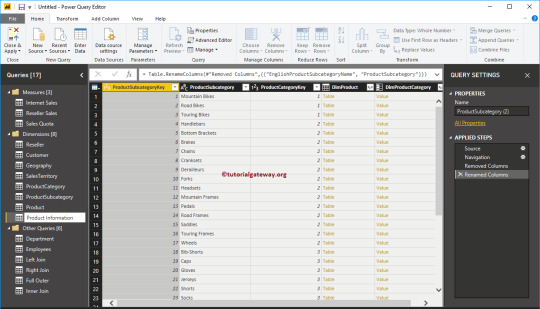
Rename the columns and the table. There are a few ways to rename a column: First, select the column, then either select Rename from the Transform tab on the ribbon, or right-click and select Rename. The following image has arrows pointing to both options; you only need to choose one.

Rename the columns to State Name and State Code. To rename the table, enter the Name in the Query Settings pane. Name this table StateCodes.

Combine queries

Now that we’ve shaped the StateCodes table the way we want, let’s combine these two tables, or queries, into one. Because the tables we now have are a result of the queries we applied to the data, they’re often referred to as queries.

Power Bi Create Table From Another Table

There are two primary ways of combining queries: merging and appending.

When you have one or more columns that you’d like to add to another query, you merge the queries.

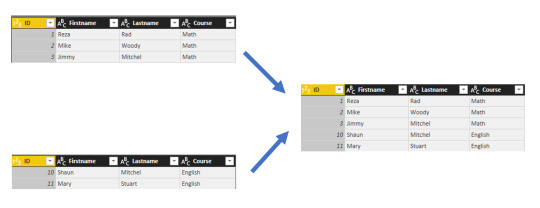
When you have additional rows of data that you’d like to add to an existing query, you append the query.

Inner Join Two Tables In Power Bi

In this case, we want to merge the queries. To do so, follow these steps:

Link Tables In Power Bi

From the left pane of Power Query Editor, select the query into which you want the other query to merge. In this case, it's RetirementStats.

Select Merge Queries > Merge Queries from the Home tab on the ribbon.

You may be prompted to set the privacy levels, to ensure the data is combined without including or transferring data you don't want transferred.

The Merge window appears. It prompts you to select which table you'd like merged into the selected table, and the matching columns to use for the merge.

Select State from the RetirementStats table, then select the StateCodes query.

When you select the correct matching columns, the OK button is enabled.

Select OK.

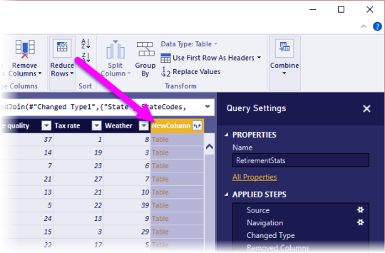
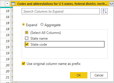
Power Query Editor creates a new column at the end of the query, which contains the contents of the table (query) that was merged with the existing query. All columns from the merged query are condensed into the column, but you can Expand the table and include whichever columns you want.

To expand the merged table, and select which columns to include, select the expand icon ().

The Expand window appears.

In this case, we want only the State Code column. Select that column, clear Use original column name as prefix, and then select OK.

From your Web browser, go to the Google Drive File Stream home page. On the Google Drive Help page, click on Download for Windows. In the following pop-up window, click Save File. If you’re prompted to enter a location in which to save the installer file, titled googledrivefilestream.exe, save the file. Access all of your Google Drive content directly from your Mac or PC, without using up disk space. Learn more Download Backup and Sync for Mac Download Backup and Sync for Windows. Download google drive stream pc. At the bottom right (Windows) or top right (Mac), click Drive for desktop Open Google Drive. When you install Drive for desktop on your computer, it creates a drive in My Computer or a location in.

If we had left the checkbox selected for Use original column name as prefix, the merged column would be named NewColumn.State Code.

Note

Want to explore how to bring in the NewColumn table? You can experiment a bit, and if you don’t like the results, just delete that step from the Applied Steps list in the Query Settings pane; your query returns to the state prior to applying that Expand step. You can do this as many times as you like until the expand process looks the way you want it.

We now have a single query (table) that combines two data sources, each of which has been shaped to meet our needs. This query can serve as a basis for many additional and interesting data connections, such as housing cost statistics, demographics, or job opportunities in any state.

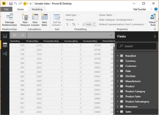
To apply your changes and close Power Query Editor, select Close & Apply from the Home ribbon tab.

The transformed dataset appears in Power BI Desktop, ready to be used for creating reports.

Cross Join Two Tables In Power Bi

Next steps

For more information on Power BI Desktop and its capabilities, see the following resources:

[blogdual890]

Combining Tables In Power Bi

Combining / Stacking / Appending Tables This is truly the easiest part, now all you need to do is find the button that reads Append Queries and then a new window will appear where you can combine all the queries that you want.

Combine Tables In Power Bi Dax

Power Bi Merge Multiple Tables

Combining Tables In Power Bi Software

Append Tables In Power Bi

Learn how to quickly merge and append tables using the query editior in Power BI. Build models with multiple data sources.Contact me on LinkedIn:www.linkedin.

I have done a few videos on YouTube explaining how to join tables using Power Query or DAX. If you follow the channel, you probably have seen the videos and this blog post will serve as a compilation of all the material. However, if you are new, this will serve as a tutorial for beginners on how to joins in Power BI.

How to join tables in power bi desktop: a practical example Combining data. When it comes to combining data in tables, it can be done in two ways. One is you may need to increase. The data set I have used for demonstration purpose is on India’s state-wise crop production collected.

-->

With Power BI Desktop, you can connect to many different types of data sources, then shape the data to meet your needs, enabling you to create visual reports to share with others. Shaping data means transforming the data: renaming columns or tables, changing text to numbers, removing rows, setting the first row as headers, and so on. Combining data means connecting to two or more data sources, shaping them as needed, then consolidating them into a useful query.

In this tutorial, you'll learn how to:

Shape data by using Power Query Editor.

Connect to different data sources.

Combine those data sources, and create a data model to use in reports.

This tutorial demonstrates how to shape a query by using Power BI Desktop, highlighting the most common tasks. The query used here is described in more detail, including how to create the query from scratch, in Getting Started with Power BI Desktop.

Power Query Editor in Power BI Desktop makes ample use of right-click menus, as well as the Transform ribbon. Most of what you can select in the ribbon is also available by right-clicking an item, such as a column, and choosing from the menu that appears.

Shape data

When you shape data in Power Query Editor, you provide step-by-step instructions for Power Query Editor to carry out for you to adjust the data as it loads and presents it. The original data source isn't affected; only this particular view of the data is adjusted, or shaped.

The steps you specify (such as rename a table, transform a data type, or delete a column) are recorded by Power Query Editor. Each time this query connects to the data source, Power Query Editor carries out those steps so that the data is always shaped the way you specify. This process occurs whenever you use Power Query Editor, or for anyone who uses your shared query, such as on the Power BI service. Those steps are captured, sequentially, in the Query Settings pane, under Applied Steps. We’ll go through each of those steps in the next few paragraphs.

From Getting Started with Power BI Desktop, let's use the retirement data, which we found by connecting to a web data source, to shape that data to fit our needs. We'll add a custom column to calculate rank based on all data being equal factors, and compare this column to the existing column, Rank.

From the Add Column ribbon, select Custom Column, which lets you add a custom column.

In the Custom Column window, in New column name, enter New Rank. In Custom column formula, enter the following data:

Make sure the status message is No syntax errors have been detected, and select OK.

To keep column data consistent, transform the new column values to whole numbers. To change them, right-click the column header, and then select Change Type > Whole Number.

If you need to choose more than one column, select a column, hold down SHIFT, select additional adjacent columns, and then right-click a column header. You can also use the CTRL key to choose non-adjacent columns.

To transform column data types, in which you transform the current data type to another, select Data Type Text from the Transform ribbon.

In Query Settings, the Applied Steps list reflects any shaping steps applied to the data. To remove a step from the shaping process, select the X to the left of the step.

In the following image, the Applied Steps list reflects the added steps so far:

Source: Connecting to the website.

Extracted Table from Html: Selecting the table.

Changed Type: Changing text-based number columns from Text to Whole Number.

Added Custom: Adding a custom column.

Changed Type1: The last applied step.

Adjust data

Before we can work with this query, we need to make a few changes to adjust its data:

Adjust the rankings by removing a column.

We've decided Cost of living is a non-factor in our results. After removing this column, we find that the data remains unchanged.

Fix a few errors.

Because we removed a column, we need to readjust our calculations in the New Rank column, which involves changing a formula.

Sort the data.

Sort the data based on the New Rank and Rank columns.

Replace the data.

We'll highlight how to replace a specific value and the need of inserting an Applied Step.

Change the table name.

Because Table 0 isn't a useful descriptor for the table, we'll change its name.

To remove the Cost of living column, select the column, choose the Home tab from the ribbon, and then select Remove Columns.

Notice the New Rank values haven't changed, due to the ordering of the steps. Because Power Query Editor records the steps sequentially, yet independently, of each other, you can move each Applied Step up or down in the sequence.

Right-click a step. Power Query Editor provides a menu that lets you do the following tasks:

Rename; Rename the step.

Delete: Delete the step.

DeleteUntil End: Remove the current step, and all subsequent steps.

Move before: Move the step up in the list.

Move after: Move the step down in the list.

Move up the last step, Removed Columns, to just above the Added Custom step.

Select the Added Custom step.

Notice the data now shows Error, which we'll need to address.

There are a few ways to get more information about each error. If you select the cell without clicking on the word Error, Power Query Editor displays the error information.

If you select the word Error directly, Power Query Editor creates an Applied Step in the Query Settings pane and displays information about the error.

Because we don't need to display information about the errors, select Cancel.

To fix the errors, select the New Rank column, then display the column's data formula by selecting the Formula Bar checkbox from the View Skype for business eol. tab.

Remove the Cost of living parameter and decrement the divisor, by changing the formula as follows:

Select the green checkmark to the left of the formula box or press Enter.

Power Query Editor replaces the data with the revised values and the Added Custom step completes with no errors.

Note

You can also select Remove Errors, by using the ribbon or the right-click menu, which removes any rows that have errors. However, we didn't want to do so in this tutorial because we wanted to preserve the data in the table.

Sort the data based on the New Rank column. First, select the last applied step, Changed Type1 to display the most recent data. Then, select the drop-down located next to the New Rank column header and select Sort Ascending.

The data is now sorted according to New Rank. However, if you look at the Rank column, you'll notice the data isn't sorted properly in cases where the New Rank value is a tie. We'll fix it in the next step.

To fix the data sorting issue, select the New Rank column and change the formula in the Formula Bar to the following formula:

Select the green checkmark to the left of the formula box or press Enter.

The rows are now ordered in accordance with both New Rank and Rank. In addition, you can select an Applied Step anywhere in the list, and continue shaping the data at that point in the sequence. Power Query Editor automatically inserts a new step directly after the currently selected Applied Step.

In Applied Step, select the step preceding the custom column, which is the Removed Columns step. Here we'll replace the value of the Weather ranking in Arizona. Right-click the appropriate cell that contains Arizona's Weather ranking, and then select Replace Values. Note which Applied Step is currently selected.

Select Insert.

Because we're inserting a step, Power Query Editor warns us about the danger of doing so; subsequent steps could cause the query to break.

Change the data value to 51.

Power Query Editor replaces the data for Arizona. When you create a new Applied Step, Power Query Editor names it based on the action; in this case, Replaced Value. If you have more than one step with the same name in your query, Power Query Editor adds a number (in sequence) to each subsequent Applied Step to differentiate between them.

Select the last Applied Step, Sorted Rows.

Notice the data has changed regarding Arizona's new ranking. This change occurs because we inserted the Replaced Value step in the correct location, before the Added Custom step.

Lastly, we want to change the name of that table to something descriptive. In the Query Settings pane, under Properties, enter the new name of the table, and then select Enter. Name this table RetirementStats.

When we start creating reports, it’s useful to have descriptive table names, especially when we connect to multiple data sources, which are listed in the Fields pane of the Report view.

We’ve now shaped our data to the extent we need to. Next let’s connect to another data source, and combine data.

Combine data

The data about various states is interesting, and will be useful for building additional analysis efforts and queries. But there’s one problem: most data out there uses a two-letter abbreviation for state codes, not the full name of the state. We need a way to associate state names with their abbreviations.

Combine Tables In Power Bi Dax

We’re in luck; there’s another public data source that does just that, but it needs a fair amount of shaping before we can connect it to our retirement table. TO shape the data, follow these steps:

From the Home ribbon in Power Query Editor, select New Source > Web.

Enter the address of the website for state abbreviations, https://en.wikipedia.org/wiki/List_of_U.S._state_abbreviations, and then select Connect.

The Navigator displays the content of the website.

Select Codes and abbreviations. Home alone on netflix streaming.

Tip

It will take quite a bit of shaping to pare this table’s data down to what we want. Is there a faster or easier way to accomplish the steps below? Yes, we could create a relationship between the two tables, and shape the data based on that relationship. The following steps are still good to learn for working with tables; however, relationships can help you quickly use data from multiple tables.

To get the data into shape, follow these steps:

Power Bi Merge Multiple Tables

Remove the top row. Because it's a result of the way that the web page’s table was created, we don’t need it. From the Home ribbon, select Remove Rows > Remove Top Rows.

The Remove Top Rows window appears, letting you specify how many rows you want to remove.

Note

If Power BI accidentally imports the table headers as a row in your data table, you can select Use First Row As Headers from the Home tab, or from the Transform tab in the ribbon, to fix your table.

Remove the bottom 26 rows. These rows are U.S. territories, which we don’t need to include. From the Home ribbon, select Remove Rows > Remove Bottom Rows.

Because the RetirementStats table doesn't have information for Washington DC, we need to filter it from our list. Select the Region Status drop-down, then clear the checkbox beside Federal district.

Remove a few unneeded columns. Because we need only the mapping of each state to its official two-letter abbreviation, we can remove several columns. First select a column, then hold down the CTRL key and select each of the other columns to be removed. From the Home tab on the ribbon, select Remove Columns > Remove Columns.

Note

This is a good time to point out that the sequence of applied steps in Power Query Editor is important, and can affect how the data is shaped. It’s also important to consider how one step may impact another subsequent step; if you remove a step from the Applied Steps, subsequent steps may not behave as originally intended, because of the impact of the query’s sequence of steps.

Note

When you resize the Power Query Editor window to make the width smaller, some ribbon items are condensed to make the best use of visible space. When you increase the width of the Power Query Editor window, the ribbon items expand to make the most use of the increased ribbon area.

Rename the columns and the table. There are a few ways to rename a column: First, select the column, then either select Rename from the Transform tab on the ribbon, or right-click and select Rename. The following image has arrows pointing to both options; you only need to choose one.

Rename the columns to State Name and State Code. To rename the table, enter the Name in the Query Settings pane. Name this table StateCodes.

Combine queries

Now that we’ve shaped the StateCodes table the way we want, let’s combine these two tables, or queries, into one. Because the tables we now have are a result of the queries we applied to the data, they’re often referred to as queries.

There are two primary ways of combining queries: merging and appending.

When you have one or more columns that you’d like to add to another query, you merge the queries.

When you have additional rows of data that you’d like to add to an existing query, you append the query.

In this case, we want to merge the queries. To do so, follow these steps:

From the left pane of Power Query Editor, select the query into which you want the other query to merge. In this case, it's RetirementStats.

Select Merge Queries > Merge Queries from the Home tab on the ribbon.

You may be prompted to set the privacy levels, to ensure the data is combined without including or transferring data you don't want transferred.

The Merge window appears. It prompts you to select which table you'd like merged into the selected table, and the matching columns to use for the merge.

Select State from the RetirementStats table, then select the StateCodes query.

When you select the correct matching columns, the OK button is enabled.

Select OK.

Power Query Editor creates a new column at the end of the query, which contains the contents of the table (query) that was merged with the existing query. All columns from the merged query are condensed into the column, but you can Expand the table and include whichever columns you want.

To expand the merged table, and select which columns to include, select the expand icon ().

The Expand window appears.

In this case, we want only the State Code column. Select that column, clear Use original column name as prefix, and then select OK.

If we had left the checkbox selected for Use original column name as prefix, the merged column would be named NewColumn.State Code.

Note

Want to explore how to bring in the NewColumn table? You can experiment a bit, and if you don’t like the results, just delete that step from the Applied Steps list in the Query Settings pane; your query returns to the state prior to applying that Expand step. You can do this as many times as you like until the expand process looks the way you want it.

We now have a single query (table) that combines two data sources, each of which has been shaped to meet our needs. This query can serve as a basis for many additional and interesting data connections, such as housing cost statistics, demographics, or job opportunities in any state.

To apply your changes and close Power Query Editor, select Close & Apply from the Home ribbon tab.

The transformed dataset appears in Power BI Desktop, ready to be used for creating reports.

Combining Tables In Power Bi Software

Next steps

Append Tables In Power Bi

For more information on Power BI Desktop and its capabilities, see the following resources:

[hostingloading4]

Merge Excel Files Tool

Merge Excel File Tool Download

Merge Excel Files Tool_v1

But for many Excel users, this task can be quite challenging and very time-consuming. The good news is, that there are several excel comparison tools available which make it very easy to merge excel files. Here are my favorite tools for merging Excel Files: Synkronizer. How to Merge Excel Files, Spreadsheets and Workbooks with Excel Merger: A Step by Step Guide Step 1: Add files to Excel Merger There are two ways of doing that. First you can drag and drop your files to the. Step 2: Set options Since you are merging files, select “Files” in the Merge dropdown. Select the excel file you want to the merge other files into. Finally, to merge Excel files, check the Create a copy checkbox, select (move to end) and click OK. Selecting (move to end), moves the excel worksheet you are merging to the end of the worksheet you are merging it into. RDBMerge, Excel Merge Add-in for Excel for Windows. RDBMerge is a user friendly way to Merge Data from Multiple Excel Workbooks, csv and xml files into a Summary Workbook. Install the RDBMerge utility. 1) Download the correct version and extract it to a local directory. 2) Copy RDBMerge.xla(m) to a unprotected directory on your system.

Choose Tools > Combine Files. The Combine Files interface is displayed with the toolbar at the top.

Drag files or emails directly into the Combine Files interface. Alternatively, choose an option from the Add Files menu. You can add a folder of files, a web page, any currently open files, items in the clipboard, pages from a scanner, an email, or a file you combined previously (Reuse Files).

Note:

If you add a folder that contains files other than PDFs, the non-PDF files are not added.

In the Thumbnail view, drag-and-drop the file or pageinto position. As you drag, a blue bar moves between pages or documentsto indicate the current position.

In the Thumbnail view, hover over the page or file and then click the Expand pages thumbnail . In expanded view, you can easily move the individual pages among the other pages and documents.

To collapse the pages, hover over the first page and then click the Collapse Document thumbnail .

In the Thumbnail view, hover over the page, and then click the Zoom thumbnail .

In the Thumbnail view, hover over the page and then click the Delete thumbnail .

In the List view, click the column name that you wantto sort by. Sigil for marriage prayer. Click again to sort in reverse order. The order of filesin the list reflects the order of the files in the combined PDF.Sorting rearranges the pages of the combined PDF.

In the List view, select the file or files you want to move. Then click the Move Up or Move Down button.

Click Options, and select one of the file size options for the converted file:

Reduces large images to screen resolution and compresses the images by using low-quality JPEG. This option is suitable for onscreen display, email, and the Internet.

Note: If any of the source files are already PDFs, the Smaller File Size option applies the Reduce File Size feature to those files. The Reduce File Size feature is not applied if either the Default File Size or Larger File Size option is selected.

Create PDFs suitable for reliable viewing and printing of business documents. The PDF files in the list retain their original file size and quality.

Creates PDFs suitable for printing on desktop printers. Applies the High Quality Print conversion preset and the PDF files in the list retain the original file size and quality.

Note:

This option may result in a larger file size for the final PDF.

In the Options dialog box, specify the conversion settings as needed, then click OK.

When you have finished arranging the pages, click Combine.

A status dialog box shows the progress of the file conversions.Some source applications start and close automatically.

Home | Products |Purchase |

Merge Excel File Tool Download

FAQ |

Contact Us | Useful Resources

Merge Excel Files Tool software can merge multiple excel sheets into one new sheet or merge excel workbooks into one new workbook with multiple worksheets. The software also can import one or more CSV files, XML files, TXT files into a blank MS Excel file, and insert them all into one sheet or individual sheets.

You may have to merge excel files into one new sheet or merge excel workbooks into one new workbook, then Merge Excel Files Tool software is your right choice in simplifying your tedious merging work. read more

Deep partial thickness burn.

Download Free Merge Excel Files Tool Please download our software and use it .

The Merge Excel Files Tool is including the technical support, unlimited software upgrades during all software life time.

Merge Excel Files Tool_v1

The software add advanced data analysis capabilities to Microsoft Excel and are guaranteed to save you time and speed up your work.With the tools you can merge, split, match, filter, remove duplicates, query, create Crosstab / Pivot Table, summarize, count , average, maximum, minimum, median, subtotal, count blank and SQL Query your data. Over 50 powerful features are included in this easy-to-use package. read more

The software can split a sheet into multiple sub sheets by the field in columns. You may have to split a very large worksheet into sub sheets by the field in columns, then the software is your right choice in simplifying your tedious splitting work. It worked smoothly and quickly, even with large worksheets, thereby saves your time. read more

The software can save each excel sheet as separate excel file. The program supports command line interface, So, you can run it with necessary parameters in a batch mode from the command line or from Windows scheduler without human beings. read more

The Software is a batch csv converter that converts Excel to CSV files. It allows you to Save one or more Excel to CSV (comma-separated values) files, also can save each sheet as an individual file.The program supports command line interface. read more

The software allows you to create SQL queries by clicking and arranging visual elements instead of writing SQL code even if you don't understand SQL. It can query Access, Excel Using SQL and execute SQL insert sheet for excel data in seconds. read more

Zoom manycam app. Connect ManyCam to Zoom. Getting Started Introduction to ManyCam. Getting started with ManyCam. ManyCam tray icon. ManyCam Main Live window. ManyCam Interface. ManyCam Video Settings - Quality & Performance. ManyCam is the go-to software to enhance your live video on streaming platform, video conferencing app and distant classes. Add multiple cameras and video sources, such as mobile and PowerPoint, use virtual backgrounds, create layers and presets, screencast desktop, and more. Zoom is the leader in modern enterprise video communications, with an easy, reliable cloud platform for video and audio conferencing, chat, and webinars across mobile, desktop, and room systems. Zoom Rooms is the original software-based conference room solution used around the world in board, conference, huddle, and training rooms, as well as executive offices and classrooms.

The software can merge excel workbooks into one new workbook with multiple worksheets Are you still bothered by the cumbersome job of merging multiple excel workbooks into one workbook? You may have to merge multiple excel sheets into one workbook, then it is your right choice in simplifying your tedious merging Work. read more

The software can Protect or Unprotect Multiple Excel Worksheets and Workbooks. It is very simple to use. It can batch Protect or Unprotect Multiple Excel Worksheets and workbooks, thereby saves your time! read more

The software can convert Excel Dates to Weekday, Month, Quarter, Year, Day of year, Hour, Minute, Second; Convert Text to Proper Case, Lower Case, Upper Case; Convert Excel Data Types to General or Text; Convert phone numbers to a uniform format; Convert ZIP to City State ZIP; Convert City, State to ZIP. read more

read more

[solsarin]

how to calculate attendance percentage in excel

how to calculate attendance percentage in excel

Hello dear friends, thank you for choosing us. In this post on the solsarin site, we will talk about “  how to calculate attendance percentage in excel “. Stay with us. Thank you for your choice.

Percent of students absent

Generic formula

=(total-attended)/total

Summary

To calculate the percentage of students absent in a given class, you can use simple formula that divides students absent (calculated by subtracting attending from total) by the total. In the example shown, the formula in E5, copied down, is:

=(C5-D5)/C5

The result is a decimal value that is formatted using the percentage number format.

Explanation

In this example, the goal is to answer the question “What percentage of students were absent from each class”. In other words, given a class with 30 students total, 27 of which were present, we want to return 10% absent. The general formula for this calculation, where “x” is the percent absent is:

x=absent/total

However, since we don’t have a column for the number of students absent in the table, we need to calculate this number as part of the formula:

x=(total-attended)/total x=(30-27)/30 x=3/30 x=0.10

After we convert this to an Excel formula with cell references, the formula in E5 becomes:

=(C5-D5)/C5 =(30-27)/30 =3/30 =0.10

As the formula is copied down, the formula returns calculated “percent absent” for each class listed in the table. These results are decimal numbers formatted with the Percentage number format.

Formatting percentages in Excel

In mathematics, a percentage is a number expressed as a fraction of 100. For example, 55% is read as “Fifty-five percent” and is equivalent to 55/100 or 0.55. To display values like this with with a percent sign (%), apply Percentage number format.

AuthorDave BrunsRelated formulasGet percentage of totalIn this example, the goal is to work out the “percent of total” for each expense shown in the worksheet. In other words, given that we know the total is $1945, and we know Rent is $700, we want to determine that Rent is 36% of the total. The total…Percent of goalIn this example, the objective is to calculate a percentage for each goal shown in column C of the table using the actual values in column D. In other words, given a goal of 100000, and an actual amount of 112000, we want to return 112% as the…Get amount with percentageIn this example, the goal is to convert the percentages shown in column C to amounts, where the total of all amounts is given as $1945. In other words, if we know Rent is 36.0%, and the total of all expenses is $1945, we want to calculate that Rent…Get percent of year completeThe goal in this example is to return the amount of time completed in a year as a percentage value, based on any given date. In other words, when given the date July 1, 2021, the formula should return 50% since we are halfway* through the year. *By…Related videos .

Random Posts

how many percentage of pure water is on earth

how much alcohol in budweiser beer

Determining your Monthly Attendance Percentage

Posted by Nancy Paulson

The Monthly Attendance Percenatge is the average of the weekly attendance for your club.

Read a section of the RI Secretary’s Manual to understand who to include in your attendance reports.

Basic Process

On a weekly basis determine the attendance percentage. (Number of Members Present or Made Up) divided by (Number of Members Used in Calculating Attendance) multiplied by 100 equals the weekly attendance percentage.

At the end of the month, average the weekly percentages to get the monthly percentage. (Sum of all the weekly percentages) divided by (Number of meetings this month) equals the monthly attendance percentage.

Methods

Use a calculator following the formulas provided above.

Use the Excel spreadsheet provided in the download files to the left. Note you must have Excel or Open Office on your computer to use this file

How to Create Attendance Tracker in Exce

Why buy an expensive attendance management tool for your startup if you can track the attendance of the team in Excel? Yes! You can create an Attendance tracker in Excel easily. In this article, we will learn how to do so.

Step1: Create 12 sheets for Every Month in a workbook

If you plan to track attendance for a year, you will need to create each month’s sheet in Excel.

Step 2: Add Columns for each date in each month’s sheet.

Now create a table that contains the names of your teammates, a column for totals and 30 (or number of days a month) columns with date and weekday as column headings.

To get the name of weekday you can look up the calendar or you can use the formula to copy it in the rest of the cells.

=TEXT(date,”ddd”)

You can read about it here.

Format the weekends and holidays dark and fill them with fixed values like Weekend/Holiday as shown in the image below.

Do the same for each sheet.

Step 3. Fix the possible inputs using data validation for each open cell.

To allow users to only write P or A for present and absent respectively, we can use data validation.

Select any cell, go to data in ribbon and click on data validation. Select list from options and write A,P in the text box.

Hit OK.

Copy this validation for the whole open range of data (open range means cell where user can insert values).

Step 3: Lock all cells except where attendance needs to be entered.

Select date a date column. For example, select 1-Jan.  Right now click on the selected range and go to the cell formatting. Go to protection. Uncheck the locked checkbox. Hit OK. Now copy this range to all open date ranges.

This will allow entry into these cells only when we protect the worksheets using worksheets protection menu. Thus your formulas, fomattings will be intact and users can only modify their attendance.

Step 4: Calculate Present Days of Teammates

So how do you calculate the present days? Well everyone has their own formulas for calculating attendance. I will discuss mine here. You can make changes as per your attendance sheet requirement.

I count the total number of present days as total days in a month, minus the number of days absent. This will keep holidays and weekends in check. They will automatically be counted as working days.

So the excel formula for counting present days will be like:

=COUNT(dates)-COUNTIF(attendance_range, “A”)

This will by default keep everyone present for the whole month until you have marked them absent on the sheet.

In the example, the formula is:

=COUNT($C$2:$AG$2)-COUNTIF(C3:AG3,”A”

Step 5: Protect the Sheet

Now that we have done everything on this sheet. Let’s protect it so that no one can alter the formula or the formatting on the sheet.

Go to the review tab in the ribbon. Find the Protect Sheet menu. Click on it. It will open a dialog box that will ask for the permissions you want to give to the users. Check all the permissions you would like to allow. I only want the user to be able to fill attendance with nothing else. So I am gonna keep it as it is.

You should use a password that you can remember easily. Otherwise, anyone can unlock it and alter the attendance workbook.

Step 6: Do  the above procedure for all the month sheets

Do the same thing for each month sheet. The best way is to copy the same sheet and make 12 sheets out of it. Unprotect them and make the necessary changes and then protect them again.

Prepare the Master Attendance Sheet

Although we have all the sheets ready to be used for attendance filling, we don’t have one place to monitor them all.

Step 7: Prepare Master Table To Monitor Attendance at one place in Excel

For that,  prepare a table that contains the name of team mates as row headings and name of month as column headings.  See the image below.

Step 7: Lookup Attendance of Team From Each Month Sheet

To look up attendance from the sheet we can have a simple VLOOKUP formula but then we will have to do it 12 times for each sheet. But you know that we can have one formula to look up from multiple sheets.

Use this formula in Cell C3 and copy in the rest of the sheets.

=VLOOKUP($A3,INDIRECT(C$2&”!$A$3:$B$12″),2,0)

Step 8: Use the Sum function to get all the present days of the year of a team mate.

This is optional. If you like you can calculate the total present days of your employees throughout the year by simply using the sum formula.

Microsoft Excel

Microsoft Excel is a spreadsheet developed by Microsoft for Windows, macOS, Android and iOS. It features calculation, graphing tools, pivot tables, and a macro programming language called Visual Basic for Applications (VBA).

resource: wikipedia

[loadingtax915]

Python Docx

Python Docx4j

Python Docx To Pdf

Python Docx Table

Python Docx To Pdf

Python Docx2txt

Python Docx2txt

When you ask someone to send you a contract or a report there is a high probability that you’ll get a DOCX file. Whether you like it not, it makes sense considering that 1.2 billion people use Microsoft Office although a definition of “use” is quite vague in this case. DOCX is a binary file which is, unlike XLSX, not famous for being easy to integrate into your application. PDF is much easier when you care more about how a document is displayed than its abilities for further modifications. Let’s focus on that.

Python-docx versions 0.3.0 and later are not API-compatible with prior versions. Python-docx is hosted on PyPI, so installation is relatively simple, and just depends on what installation utilities you have installed. Python-docx may be installed with pip if you have it available.

Installing Python-Docx Library Several libraries exist that can be used to read and write MS Word files in Python. However, we will be using the python-docx module owing to its ease-of-use. Execute the following pip command in your terminal to download the python-docx module as shown below.

Python has a few great libraries to work with DOCX (python-dox) and PDF files (PyPDF2, pdfrw). Those are good choices and a lot of fun to read or write files. That said, I know I'd fail miserably trying to achieve 1:1 conversion.

Release v0.8.10 (Installation)python-docx is a Python library for creating and updating Microsoft Word (.docx) files.

Looking further I came across unoconv. Universal Office Converter is a library that’s converting any document format supported by LibreOffice/OpenOffice. That sound like a solid solution for my use case where I care more about quality than anything else. As execution time isn't my problem I have been only concerned whether it’s possible to run LibreOffice without X display. Apparently, LibreOffice can be run in haedless mode and supports conversion between various formats, sweet!

I’m grateful to unoconv for an idea and great README explaining multiple problems I can come across. In the same time, I’m put off by the number of open issues and abandoned pull requests. If I get versions right, how hard can it be? Not hard at all, with few caveats though.

Testing converter

LibreOffice is available on all major platforms and has an active community. It's not active as new-hot-js-framework-active but still with plenty of good read and support. You can get your copy from the download page. Be a good user and go with up-to-date version. You can always downgrade in case of any problems and feedback on latest release is always appreciated.

On macOS and Windows executable is called soffice and libreoffice on Linux. I'm on macOS, executable soffice isn't available in my PATH after the installation but you can find it inside the LibreOffice.app. To test how LibreOffice deals with your files you can run:

In my case results were more than satisfying. The only problem I saw was a misalignment in a file when the alignment was done with spaces, sad but true. This problem was caused by missing fonts and different width of 'replacements' fonts. No worries, we'll address this problem later.

Setup I

While reading unoconv issues I've noticed that many problems are connected due to the mismatch of the versions. I'm going with Docker so I can have pretty stable setup and so I can be sure that everything works.

Let's start with defining simple Dockerfile, just with dependencies and ADD one DOCX file just for testing:

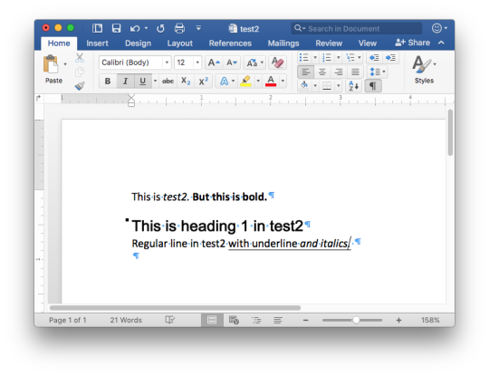
Let's build an image:

After image is created we can run the container and convert the file inside the container:

Running LibreOffice as a subprocess

We want to run LibreOffice converter as a subprocess and provide the same API for all platforms. Let's define a module which can be run as a standalone script or which we can later import on our server.

Required arguments which convert_to accepts are folder to which we save PDF and a path to the source file. Optionally we specify a timeout in seconds. I’m saying optional but consider it mandatory. We don’t want a process to hang too long in case of any problems or just to limit computation time we are able to give away to each conversion. LibreOffice executable location and name depends on the platform so edit libreoffice_exec to support platform you’re using.

subprocess.run doesn’t capture stdout and stderr by default. We can easily change the default behavior by passing subprocess.PIPE. Unfortunately, in the case of the failure, LibreOffice will fail with return code 0 and nothing will be written to stderr. I decided to look for the success message assuming that it won’t be there in case of an error and raise LibreOfficeError otherwise. This approach hasn’t failed me so far.

Uploading files with Flask

Converting using the command line is ok for testing and development but won't take us far. Let's build a simple server in Flask.

We'll need few helper function to work with files and few custom errors for handling error messages. Upload directory path is defined in config.py. You can also consider using flask-restplus or flask-restful which makes handling errors a little easier.

The server is pretty straightforward. In production, you would probably want to use some kind of authentication to limit access to uploads directory. If not, give up on serving static files with Flask and go for Nginx.

Important take-away from this example is that you want to tell your app to be threaded so one request won't prevent other routes from being served. However, WSGI server included with Flask is not production ready and focuses on development. In production, you want to use a proper server with automatic worker process management like gunicorn. Check the docs for an example how to integrate gunicorn into your app. We are going to run the application inside a container so host has to be set to publicly visible 0.0.0.0.

Setup II

Now when we have a server we can update Dockerfile. We need to copy our application source code to the image filesystem and install required dependencies.

In docker-compose.yml we want to specify ports mapping and mount a volume. If you followed the code and you tried running examples you have probably noticed that we were missing the way to tell Flask to run in a debugging mode. Defining environment variable without a value is causing that this variable is going to be passed to the container from the host system. Alternatively, you can provide different config files for different environments.

Supporting custom fonts

I've mentioned a problem with missing fonts earlier. LibreOffice can, of course, make use of custom fonts. If you can predict which fonts your user might be using there's a simple remedy. Add following line to your Dockfile.

Now when you put custom font file in the font directory in your project, rebuild the image. From now on you support custom fonts!

Summary

This should give you the idea how you can provide quality conversion of different documents to PDF. Although the main goal was to convert a DOCX file you should be fine with presentations, spreadsheets or images.

Further improvements could be providing support for multiple files, the converter can be configured to accept more than one file as well.

Photo by Samuel Zeller on Unsplash.

Did you enjoy it? Follow me@MichalZalecki on Twitter, where I share some interesting, bite-size content.

This ebook goes beyond Jest documentation to explain software testing techniques. I focus on unit test separation, mocking, matchers, patterns, and best practices.

Get it now!

Mastering Jest: Tips & Tricks | $9

Latest version

Released:

Extract content from docx files

Project description

Extract docx headers, footers, text, footnotes, endnotes, properties, and images to a Python object.

The code is an expansion/contraction of python-docx2txt (Copyright (c) 2015 Ankush Shah). The original code is mostly gone, but some of the bones may still be here.

shared features:

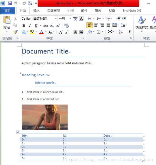
extracts text from docx files

extracts images from docx files

no dependencies (docx2python requires pytest to test)

additions:

extracts footnotes and endnotes

converts bullets and numbered lists to ascii with indentation

converts hyperlinks to <a href='http:/...'>link text</a>

retains some structure of the original file (more below)

extracts document properties (creator, lastModifiedBy, etc.)

inserts image placeholders in text ('----image1.jpg----')

inserts plain text footnote and endnote references in text ('----footnote1----')

(optionally) retains font size, font color, bold, italics, and underscore as html

extract user selections from checkboxes and dropdown menus

full test coverage and documentation for developers

subtractions:

no command-line interface

will only work with Python 3.4+

Installation

Use

Note on html feature:

font size, font color, bold, italics, and underline supported

hyperlinks will always be exported as html (<a href='http:/...'>link text</a>), even if export_font_style=False, because I couldn't think of a more cononical representation.

every tag open in a paragraph will be closed in that paragraph (and, where appropriate, reopened in the next paragraph). If two subsequenct paragraphs are bold, they will be returned as <b>paragraph q</b>, <b>paragraph 2</b>. This is intentional to make each paragraph its own entity.

if you specify export_font_style=True, > and < in your docx text will be encoded as > and <

Return Value

Function docx2python returns an object with several attributes.

header - contents of the docx headers in the return format described herein

footer - contents of the docx footers in the return format described herein

body - contents of the docx in the return format described herein

footnotes - contents of the docx in the return format described herein

endnotes - contents of the docx in the return format described herein

document - header + body + footer (read only)

text - all docx text as one string, similar to what you'd get from python-docx2txt

properties - docx property names mapped to values (e.g., {'lastModifiedBy': 'Shay Hill'})

images - image names mapped to images in binary format. Write to filesystem with

Return Format

Some structure will be maintained. Text will be returned in a nested list, with paragraphs always at depth 4 (i.e., output.body[i][j][k][l] will be a paragraph).

If your docx has no tables, output.body will appear as one a table with all contents in one cell:

Table cells will appear as table cells. Text outside tables will appear as table cells.

To preserve the even depth (text always at depth 4), nested tables will appear as new, top-level tables. This is clearer with an example:

becomes ...

This ensures text appears

only once

in the order it appears in the docx

always at depth four (i.e., result.body[i][j][k][l] will be a string).

Working with output

This package provides several documented helper functions in the docx2python.iterators module. Here are a few recipes possible with these functions:

Some fine print about checkboxes:

MS Word has checkboxes that can be checked any time, and others that can only be checked when the form is locked.The previous print as. u2610 (open checkbox) or u2612 (crossed checkbox). Which this module, the latter willtoo. I gave checkboxes a bailout value of ----checkbox failed---- if the xml doesn't look like I expect it to,because I don't have several-thousand test files with checkboxes (as I did with most of the other form elements).Checkboxes should work, but please let me know if you encounter any that do not.

Release historyRelease notifications | RSS feed

1.27.1

1.27

1.26

Python Docx4j

1.25

1.24

1.23

1.22

1.21

1.19

1.18

1.17

1.16

1.15

1.14

1.13

1.12

1.11

1.2

Python Docx To Pdf

1.1

Python Docx Table

1.0

0.1

Python Docx To Pdf

Download files

Download the file for your platform. If you're not sure which to choose, learn more about installing packages.

Python Docx2txt

Files for docx2python, version 1.27.1Filename, sizeFile typePython versionUpload dateHashesFilename, size docx2python-1.27.1-py3-none-any.whl (22.9 kB) File type Wheel Python version py3 Upload dateHashesFilename, size docx2python-1.27.1.tar.gz (33.3 kB) File type Source Python version None Upload dateHashes

Close

Hashes for docx2python-1.27.1-py3-none-any.whl

Hashes for docx2python-1.27.1-py3-none-any.whlAlgorithmHash digestSHA25651f6f03149efff07372ea023824d4fd863cb70b531aa558513070fe60f1c420aMD54b0ee20fed4a8cb0eaba8580c33f946bBLAKE2-256e7d5ff32d733592b17310193280786c1cab22ca4738daa97e1825d650f55157c

Close

Hashes for docx2python-1.27.1.tar.gz

Python Docx2txt

Hashes for docx2python-1.27.1.tar.gzAlgorithmHash digestSHA2566ca0a92ee9220708060ece485cede894408588353dc458ee5ec17959488fa668MD5759e1630c6990533414192eb57333c72BLAKE2-25684783b70aec51652a4ec4f42aa419a8af18d967b06390764527c81f183d1c02a

[themepluginpro]

Download ZF WordPress Category Search on Codecanyon

Description ZF WordPress Category Search :

Download ZF WordPress Category Search. The theme releases on Tuesday 21st October 2014 By The author zufusion on Codecanyon. It’s uses with author,auto suggest,custom post type,date range,dropdown category,easy digital downloads,multiple taxonomies,price range,radio category,tab category search,tab slider category,woocommerce attributes,woocommerce search,wordpress category search. Item Title: ZF WordPress Category Search Category: wordpress/ecommerce Price: $15 Author: zufusion Published Date: Tuesday 21st October 2014 03:02:13 AM More Info / DownloadDemo

ZF WordPress Category Search is a WordPress advanced search box, the ability display categories as tabs/radio/dropdown with advanced fields, support WooCommerce, Easy Digital Downloads, custom post type, taxonomies.

You can search by search categories, tags, taxonomies, authors, date range, sort, order by …

Otherwise, you can also search multiple taxonomies of custom post type. These easily to really refine your searches.

Key Features:

Tab slider category

Add icon popover for tab icon

Tab alignment

Radio category search

Dropdown category search

Auto suggest like google

Support WooCommerce category search, WordPress category search

Support Easy Digital Downloads, custom post type

Drap vs drop taxonomies to display

Search multiple taxonomies, author, price range, date range, order

Translation ready

Widget vs Shortcode ready

Easy to setup and customize

Support dark vs light skin

Cross-browser support

Change Log:

02.10.2019 - Version 2.6 * Work with WordPress 5.2

25.05.2015 - Version 2.5 * Fixed can't open advanced box when category box is empty * Fixed doesn't respond to the tags, categories of post in advanced box * Change default value of min count selected to 0 instead of 3 (only dropdown mode)

25.03.2015 - Version 2.4 * Added match type taxonomy values (categories) on setting page * Allows show open advanced button inside or outside input query * Show advanced button with icon or text or both * Fixed dropdown mode doesn't show categories * Fixed conflict with user pro plugin * Fixed long category name for dropdown mode

23.03.2015 - Version 2.3 . this version you need to save setting page again * Support search form template * Added taxonomy checkbox field * Put Advanced box inside the popup * Unlimited Level Sub Categories

02.02.2015 - Version 2.2 * Fixed menu disappear after using search * Fixed insert icon for Easy Digital Downloads

28.01.2015 - Version 2.1 * Support Easy Digital Downloads * Fixed radio css

04.11.2014 - Version 2.0 * Added auto suggest like google. * Support custom post type, multiple taxonomies * Drap vs drop taxonomies * Moved all options to setting page. * Added some hooks function for the developer.

More Info / DownloadDemo #WordPress #Category #Search

[hydrus]

Version 446

windows

zip

exe

macOS

app

linux

tar.gz

I had an ok week. The client does not have a huge changelog this week, but the server has a neat privacy improvement.

The PTR is going to be doing a heap of maintenance this week. It will be 'busy' a lot, approximately one hour of busy and then three hours free. Please bear with it, and if you have a million mappings to upload, I recommend you just give it a break and come back later. I am not totally sure how long it will take. Best case it is a day, worst case it might take four or five.

null account

tl;dr: The hydrus server is now even more anon. You don't have to do anything.

As the PTR has moved to multiple accounts, we've had several good discussions about privacy. Separate accounts, despite being anon, could potentially leave a fingerprint of preferences on the server. If the server were to fall into bad hands many years from now, someone could mine those records--maybe mixed with one time you casually said 'yeah, I added that sibling'--and perhaps derive something from it.

There is no technical need to remember which account uploaded what long term, so now all hydrus servers completely anonymise their content after a certain duration, default 90 days. A new non-useable 'null' account takes possession of files, tag mappings, siblings, or parents after the delay, letting the original uploaders be forgotten. Janitors will still have time to work on recent account-based problems, but the historical record works just like the old shared public account: all merged together.

I have updated the privacy document in the help to talk a little about it. As long as you do not tag your own face in pictures or something, I think we are pretty great now, especially if you use a VPN.

https://hydrusnetwork.github.io/hydrus/help/privacy.html#account_history

It will take some time to anonymise the PTR or any other big server, as it has to go through its whole historical record to catch up. Please bear with it.

full list

misc:

fixed a typo bug in the latest pending upload routine when it was cancelled/errors out early

fixed a problem with the new subscription gap downloader, where when the page opens with the first query, it could sometimes assign 'already in db' to items in that query that were actually 'successful'. some other downloaders may have been rarely hit by this, but it was mostly the gap downloader

the client _should_ now support a service host that has path components (e.g. one hosted on a proxy), like myserver.com/hydrus_repo. the port will now be correctly inserted in the address before all requests. hydrus and ipfs both should work, fingers crossed

when an admin modifies the account types, the server now only prints the 'updated account type' log record if there were actual changes

.

downloader UI:

the confusingly named 'file import status' and 'gallery search log' in the downloader system are now renamed 'file log'/'search log'/'check log' for the file import queue, gallery downloader, and watcher respectively. the 'table' bitmap buttons are also replaced with simple easy (and easy to refer to!) label buttons.

when you open the file/search/check logs from the downloader page list right-click menu, they now spawn properly inside regular windows, not modal dialogs (which were inhibiting interaction with the rest of the program while open)

relabelled the awkward 'even if url/hash recognised' checkboxes in file import options. 'do not skip if' becomes 'force download even if', and the text matches that in tag import options for page content. also improved the tooltip on these checkboxes

all of the downloader layout boxes have also been renamed and harmonised with each other. gone are overly technical 'import queue' and 'gallery parsing'. now it is generally 'imports' up top and 'search' or 'checker' etc... below

layouts have also been harmonised a little. the url downloader page now has boxes for file vs search URLs, the hard drive import pause button is moved up as other pages have, and several off-by-a-pixel sizer layouts have been fixed

.

null account:

to further improve server privacy, particularly after the PTR's multiple account switch, all repositories now forget which accounts uploaded which content after a certain age. by default it is 90 days, but you can check in _review services_ once a server updates. this defends against a variety of hypothetical attacks where someone very clever gains access to the raw server database files, maybe years from now, and tries to crawl its anonymous account history for derivable information--now there is no history!

it will take some time to retroactively scrub a huge server like the PTR. for the PTR, it is mostly a relative no-op of moving account ids from the old public shared account to a new 'null' account, but it'll still be about 1.2 billion rows! this happens in the background, so the server will still be useable most of the time, but it will have spikes of 'busy' for about one hour every four (i.e. one hour of mostly busy, three hours of free), probably for several days. it may be a pain to try uploading a bunch of stuff in that time, so if you have a million pending mappings, you might like to just give the PTR a break for a few days. once it has fully caught up, the anonymisation should only be 20-60 seconds of 'busy' a day

the way the anonymisation works is all serverside services now have a single non-useable 'null account' that will take possession of all content after the delay. the original uploader is lost, and the whole historical record is merged together.

the privacy help doc has been updated to talk about the new anonymising system. overall, I think the null account pretty much eliminates the speculative account cross-referencing worries we had, and I am happy

.

admin/janny info:

for admins, all repositories now have an 'anonymisation period' option that you can edit in the service admin menu, defaulting to 90 days (min 1, max 360). you'll also see summary statements in the server logs as updates are anonymised. anonymisation will kick in two minutes after boot, so if you want to change this value immediately on update, get ready and be quick about it!

for jannies who can see accounts, you will see the null account pop up in reference to older content (moreso in future when I expand janny UI and permissions). it being special is highlighted, and various account modifying UI shows it cannot be edited

also for jannies/admins, I had to do some wickity woo to get the null account to work without a network update for everyone. if you try to look at the null account on 445 you may get an error. normal users won't run into this, but there's a kind of 'soft' network version update for you today

next week

The null account took most of my time this week, and I now have several extra little jobs to catch up with. So I'll bash away at that small work, and I'd really like to crack the multiple column lists that keep growing in width.

[erossiniuk]

Create a Positive/Negative bar chart in Excel

In this post I want to explain step by step how to create a positive/negative bar chart in Microsoft Excel. Another interesting post for Excel is here about how to highlight content.

If you want to show how multiple units does comparison to each other based on the same criteria clearly, you can use the positive negative bar chart which can display positive and negative development very good as below screenshot shown.

Table of contents

Arrange data

Create chart

Adjust chart

Positive/Negative bar chart in Excel Positive/Negative bar chart in Excel

Arrange data

Supposing the original data displayed as below:

Firstly, add some helper columns:

Calculate the difference between two columns (Column C and Column B). In cell D2, type this formula

=C2-B2

Drag fill handle down to calculate the differences.

Calculate the increase or decrease percentage. In cell E2, type this formula

=D2/B2

Drag fill handle down to fill cells with this formula

Then keep cells selected, click Home tab, and go to the Number group, choose Percent Style button to format the cells shown as percentage.

Calculate the positive value and negative value. In cell F2, type this formula

=IF(E2>0,E2,NA())

E2 is the percentage cell, drag fill handle down to fill the cells with this formula.

In Cell G2, type this formula

=IF(E2<0,E2,NA())

E2 is the percentage cell, drag fill handle down to fill the cells with this formula.

Now, select F2: G9, click Home > Percent Style to format these cells as percentages.

Create chart

Now create the positive negative bar chart based on the data.

Select a blank cell, and click Insert > Insert Column or Bar Chart > Clustered Bar

Right click at the blank chart, in the context menu, choose Select Data.

In the Select Data Source dialog, click Add button to open the Edit Series dialog. In the Series name textbox, choose the Percentage header, then in the Series values textbox, choose E2:E9 that contains increasing and decreasing percentages, click OK.

Back to the Select Data Source dialog, click Add to go to the Edit Series dialog again, select F1 as the series name, and F2:F9 as the series values. F2:F9 are the positive values, Click OK.

Again, Click Add in the Select Data Source dialog to go to the Edit Series dialog, select G1 as series name, G2:G9 as series values. Click OK.

Back to the Select Data Series dialog, click Edit button in the Horizontal (Category) Axis Labels section, and choose A2:A9 as the axis label names in the Axis Labels dialog, click OK > OK to finish the select data.

Now the chart is displayed as below:

Then select the blue series, which express the increasing and decreasing percentage values, click Delete to remove them.

Adjust chart

Then adjust the chart.

Right click at the axis labels, then choose Format Axis from context menu, and in the popped Format Axis pane, check Categories in reverse order checkbox in Axis Options section, and scroll down to the Labels section, choose Low from the drop-down list beside Label Position.

Remove gridlines and X (horizontal) axis.

Right click at one series to select Format Data Point from the context menu, and in the Format Data Point pane, adjust Series Overlap to 0%, Gap Width to 25%.

Right click at left series, and click Add Data Label > Add Data Labels. 

Remove the #N/A labels one by one.

Select the chart to show the Design tab, and under Design tab, click Add Chart Element > Gridlines > Primary Major Horizontal.

You can change the series color and add chart title as you need.

This normal way can create the positive negative bar chart, but it is troublesome and takes much time. For users who want to quickly and easily handle this job, you can try below method.

If you want the file to create a Positive/Negative bar chart in Excel, visit the download section.

The post Create a Positive/Negative bar chart in Excel appeared first on PureSourceCode.

from WordPress https://www.puresourcecode.com/tips-tricks/create-a-positive-negative-bar-chart-in-excel/

[sourabhdubey007]

How To Use Calculator Plugins in WordPress

Now if you came to this post you are probably in the market, or having been considering getting, a calculator plugin but you are probably unaware of how detailed some of them can be and that deciding which one to get, may take more thought then you were thinking.  There are many types of WordPress plugins to calculate prices, measurements, dates, form fields, and more. In this article, we have hand-picked some of the best calculator plugins for WordPress. It is possible by the backend code of calculation. And for those folks who are not that expert in manual calculator coding. Then, here is the list of the best WordPress calculator plugins that lets you create a calculator on your website with no efforts.

Best Calculator Plugins

Calculated Fields Form

Calculated Fields Form can be used for creating both single and complex calculations, for example, general calculators, ideal weight calculators, calorie calculators, calculate quotes for hotel booking and rent a car service, calculate quotes for appointments and services, loan & finance calculators, date calculators. It comes with a form and logic builder which you can use to add fields, assign values to those fields, and define mathematical operators to run. It has Five pre-built samples. It has a Predefined forms template. It has a feature that Calculated fields can be hidden fields. It allows integration with Classic WordPress Editor, Gutenberg Editor, Elementor, Page Builder by SiteOrigin, Beaver Builder, WPBakery Page Builder, DIVI Builder, For other editors, the shortcodes should be inserted using other controls of general-purpose like the controls for inserting HTML or shortcodes.

Features

Visual form builder available  with multiple fields and form formatting options

Multiple numbers of calculated fields can be added like drop-down, checkboxes, radio buttons, dates, numbers

The calculator supports both easy and advanced operations, including ternary operators and common Math functions

Smart automatic number and prices identification into the field values

Supports form separators and comments sections to layout the form in a friendlier way

Practical “clone” button to duplicate a form

Conditional rules supported. Useful for creating wizards

Responsive Mortgage Calculator

If you run a real estate website, it makes sense to display calculators and other useful tools on your website. Responsive Mortgage Calculator is a simple widget that lets your visitors estimate their mortgage payments. The Responsive Mortgage Calculator is a jQuery widget and shortcode that’s designed to fit easily into any theme, on any device, at any size. There are settings to adjust the styling, a light and a dark theme, or you can remove the styling entirely and use your theme’s styling. The HTML is built with plenty of classes, so it’s easy to override the included stylesheet with your own CSS.

Features

the total cost of the home,

a down payment amount,

an interest rate (fixed rate),

the amortization period,

and they can select a payment period, either monthly, bi-weekly, or weekly,

NEW * beautiful popup summary with chart and amortization schedule.

Cost Calculator Builder

Cost Calculator – if you’re searching for a smart, simple tool that allows you to easily create price estimation forms to give your clients the opportunity to get information about your services and product costs you are in the right place. This plugin is clean and simple and it will help you to do things like: get a simple quote, project price, or estimation so then you can create a quote or price estimation form for your site. Cost Calculator is basically a WordPress plugin for quotations, price, and project estimation. This plugin allows you to easily create price estimation forms for your WordPress website. This has a textbox. It has dropdown menus with images of icons. It also has a numeric slider, on/off switcher and reCAPTCHA.   The possibilities are unlimited. Let the Cost Calculator become your virtual assistant and increase the conversion of your website.

Features

Switch Box

Input box

Checkbox

Advanced dropdown Box

Range Slider

Quantity Box

Textbox

Horizontal Line

One-click import

Responsive design

Tons of different demos

Numeric sliders

CT Mortgage Calculator

A straightforward and simple responsive mortgage calculator with a clean flat design, featuring Sale Price, Interest Rate, Term (years) & Down Payment.

Features

Responsive– mortgage calculator looks good on any device from both sides: admin and front.

Customizable  Fields-simple calculator with Purchase price, Down payment, Interest Rate or enable advanced options and switch on extra Home Insurance, Property taxes and PMI.

Nice Font– Adapt calculator color according to your theme styles. Choose any color you need via plugin Settings.

Smart-The plugin has a comprehensive interface and easy in use. Just give it a try and enjoy!

Visually attractive-The calculator displays results in the Popup window with graph or simple text. You can select one of the options most appealing for you.

To make it more attractive we used jQuery and Google Charts in its code it has jQuery animation effect

Mortgage Calculator

Mortgage Calculator WordPress Plugin is based on and uses the code from the very popular Mortgage Calculator. Not only will the plugin calculate the monthly payment amount, it can also solve for the affordable house price or calculate the down payment percentage.A mortgage calculator is a useful tool for real estate websites because it allows visitors to see if they can afford the property they’re looking at. If you are making a real website with IDX property listings, then a mortgage calculator will help you get more leads and increase user engagement on your website. Additionally, the calculator will optionally consider loan points, property taxes, hazard insurance and private mortgage insurance (PMI).  Your site visitors can select their own currency and date convention which is ideal if the host site attracts visitors from around the globe. The website or blog owner can select from four predefined sizes or modify a CSS file to customize both size and colors.

The post How To Use Calculator Plugins in WordPress appeared first on The Coding Bus.

from WordPress https://ift.tt/2MLIRZU via IFTTT

[enterinit]

Office Insider for Windows Version 2004 release notes

Office Insider for Windows Version 2004 release notes.

Build 12730.20024 (April 10, 2020)

Excel, Word, Outlook, and PowerPoint     Introducing premium creative content    Office 365 subscribers can now easily add high quality, curated images, stickers, and icons to their personal or professional documents, files, and presentations in Excel, Word, Outlook and PowerPoint. Search from more than 8,000 royalty-free images and icons with more to come!   How it works: 1. Select Insert > Pictures > Stock Images.   2. Select the content type you want to explore: Stock Images, Cutout People, Icons, or Stickers.    3. Enter some keywords in the Search box.    4. Select the image you want and select Insert.  Learn more. Word   Private Annotations Private Annotations is a way for you to easily create a Private Copy of shared documents for your personal annotations. This allows you the time and space to collect your thoughts, and thoroughly review a document on your own.   Learn more. 

Notable fixes: We fixed an issue where hovering a cursor over a ScreenTip would not highlight its card.We fixed an issue where the text in grouped shapes would temporarily disappear when using the Lasso tool.We fixed an issue where if a paragraph whose style is an ancestor of a style linked to a list, then the numbering of that list could be lost.We fixed an issue where when a user was creating a comment, the comment anchor didn't come into view when the document was in two page view. We fixed an issue where the rendering of a legacy Excel chart embedded as an OLE (object linking and embedding) in Word did not always display the chart title. PowerPoint   Synchronize changes while you are presenting For years, PowerPoint didn’t allow changes made to slides by others to be displayed while presenting. However, while some presenters may still desire this design, we’ve heard from others that they are seeking more flexibility. We’re excited to make available the ability to synchronize changes whenever they are made, even when the presentation is in Slide Show mode. Learn more. 

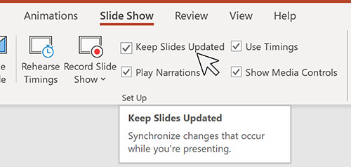
Notable fixes: We fixed an issue where copying text from Excel to PowerPoint could change the formatting.We fixed an issue where finding special characters using "find whole words only" didn't always work. We fixed an issue where the rendering of a legacy Excel chart embedded as an OLE (object linking and embedding) in PowerPoint did not always display the chart title. Access   New Add Tables pane Navigating tables and queries to establish relationships just got easier in Access! The new Add Tables pane will increase your productivity when you’re developing and viewing relationships and provide an enhanced querying experience.   How it works: 1. Select Database Tools > Relationships.    2. The Add Tables pane should appear to the right of the screen. If it does not, right-click and select Show Tables, and it will appear.   

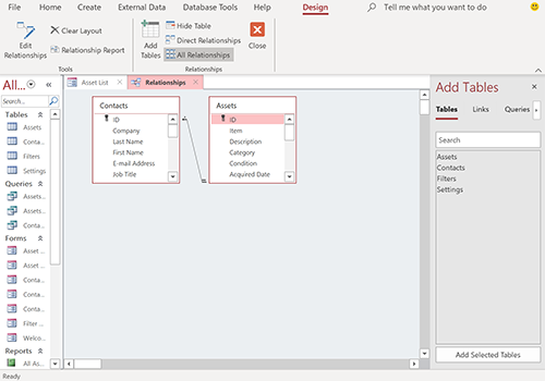
Excel  Notable fixes: We fixed an issue where selecting a range of cells on a sheet would result in the selection of a single cell.We fixed an issue where Excel would stop responding when users were reducing the size of a chart with some x-axis ranges.We fixed an issue where Data Labels on charts would display as blank when the underlying data cells did not have a caption.We fixed an issue where inserting a user defined chart template as default would result in saving it as a column chart.We fixed an issue where hovering over the user presence icon didn’t display the active cell reference in R1C1 mode in an Excel sheet that was R1C1 cell referencing enabled and shared. Outlook    High resolution photos in email   Previously when users would insert an image into an Outlook message, the photo would be converted to 96 ppi resolution. This new feature does not convert the images to a smaller size and instead adds your PNG, JPEG, BMP, GIF images to your message at their original resolution.   Notable fixes: We fixed an issue where some reminders failed to launch when the time zone was changed on a machine.We fixed an issue where users experience a crash when attempting to view the properties of an Organizational Forms Library.We fixed an issue where categories would occasionally disappear from messages. We fixed an issue where delegates would see different folder hierarchies on different machines for shared mailboxes. Project Notable fixes: We fixed an issue that was preventing users from entering time-phased Baseline Work when the setting to protect actual work was on.

Build 12718.20010 (March 27, 2020)

Outlook   Disable @ mentions Some of you have been quite vocal about wanting the ability to disable @ mentions in Outlook. We heard you and are happy to let you know that now you can do so! How it works: Select File > Options > Mail.Under Send Messages, clear the Suggest names to mention when I use the @ symbol in a message check box.Click OK. Learn more

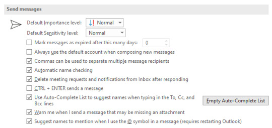
Notable fixes: We fixed an issue where Outlook didn’t show a user’s Signature list when the user was replying to a digitally rights managed message that they didn’t have owner permission for.We fixed an issue where users were unable to add additional attachments to a previously created meeting when accessing it from a web location.We fixed an issue where Save to Cloud was missing from the Attachments menu. Word  Notable fixes: We fixed an issue where the Comments pane could be empty when a user selected Multiple Pages in the View menu. PowerPoint  Notable fixes: We fixed an issue where PowerPoint files containing emojis would fail to save. Project  Notable fixes: We fixed an issue where when Custom Field Value List Get Item was executed without a lookup table for the custom field, Project would create an empty lookup table.

Build 12711.20000 (March 20, 2020)

Outlook Outlook’s Calendar gets a refresh After the successful refreshing of the mail experience last year, it was the calendar's turn to get a facelift. Thanks to your feedback, we were able to implement updates that are fresh but familiar, so seasoned Outlook users, like you, can immediately be more productive. Check out the screenshot below to take a look at some of the updates: bold headers, calendar-colored outlines, a new time indicator bar, and badges. Learn more.

Notable fixes: We fixed an issue where users were experiencing delays when processing linked images with incorrect URLs.We fixed an issue where the latest changes to draft emails were not being updated.We fixed an issue where right clicking a file and selecting Send to would not work.We fixed an issue where when a user had a customized search path for the Address book, Outlook's name resolution scope would be limited to the customized path rather than including the Global Address List.We fixed an issue where within a set of returned search results, sorting the results by Categories would not display the category colors. PowerPoint  Synchronize changes while presenting For years, PowerPoint did not allow any changes to be saved to slides while a presentation was in progress to ensure that the presenter was in full control of the content. With an increased focus on collaboration and real-time updates, customers have asked that changes be synch’ed whenever they are made, even when the presentation is in Slide Show mode. How to access: You can synchronize your presentation content in two ways. Automatically update slide content 1. Select the Keep Slide Updated checkbox on the Slide Show tab on the ribbon.

2. Start the presentation by selecting the appropriate button on the Slide Show tab.

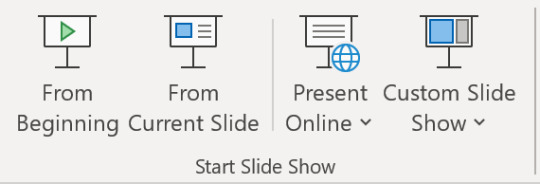
3. Whenever an update to a slide is made and detected, the content is automatically updated and visible in the slide show being presented. Manually update slide content 1. Clear the Keep Slide Updated checkbox on the Slide Show tab on the ribbon. 2. Start the presentation by selecting the appropriate button on the Slide Show tab. 3. Whenever an update to a slide is made and detected, an Update Slides button appears at the top of Presenter View.

4. Click the Update Slides button to manually synchronize the slide content. Word  Notable fixes: We fixed an issue where the functionality to post comments was disabled.We fixed an issue where users were experiencing delays when processing linked images with incorrect URLs.We fixed an issue where the account manager was not sending messages and causing third-party applications to freeze.We fixed an issue where the Table of Contents was getting updates to heading styles that did not exist in the document.We fixed an issue where digital signatures saved in Word documents would be removed when mailing the documents. Excel  Notable fixes: We fixed an issue where users were experiencing delays when processing linked images with incorrect URLs. Project  Notable fixes: We fixed an issue where the latest values for the Actual Cost of Work Performed would not be displayed after making an edit, such as a date change.We fixed an issue where opening a project using the Most Recently Used menu opened the project file with Read/Write access.We fixed an issue where when a manual task created with a start date and time, but no duration would be displayed with an incorrect time on the timeline.We fixed an issue where printing a timeline using a Hijri calendar would result in a month being skipped or duplicated in the print view. We fixed an issue where working in Team Planner with GDI objects could result in the over-allocation of GDI objects and create low memory conditions.We fixed an issue where "ProjectBeforeTaskChange" did not open when a user clicked the Inactivate button in the Schedule group after selecting a task.We fixed an issue where "ProjectBeforeTaskChange" didn't always save the changes made within a Form type view.

Build 12703.20010 (March 13, 2020)

Word, Excel, PowerPoint, and Outlook Apply a sensitivity label: You can now apply a sensitivity label that your organization has configured to prompt you for custom permissions. Sensitivity labels let you classify and protect your organization's data, while making sure that your productivity and your ability to collaborate isn’t hindered.  How to access: If your organization has set up Sensitivity labels in Microsoft Information Protection and enabled users to assign permissions, you will be able to access them. For example, select Home > Protect and select the label you want to apply to the document, workbook, presentation, or email.

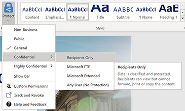
Outlook  Notable fixes: We fixed an issue that was causing the "last modified" date on a file to be updated when it was added as an attachment or when an attachment was saved by dragging and dropping it.We fixed an issue that prevented users from pressing ENTER in the expanded Find pane to start a search.We fixed an issue where search was showing no information about users when the Show user photographs when available checkbox was cleared. Word  Notable fixes: We fixed an issue when typing or editing a comment and pressing Ctrl+A would result in selecting text in the canvas instead of selecting text in the comment card.We fixed an issue where the document contents were misaligned after it had been printed using Quick Print.We fixed an issue that was preventing users from merging two documents into one.We fixed an issue where a document that contained equations with tracked changes would not save. Excel  Notable fixes: We fixed an issue that was causing delays when users were programmatically editing a large range of cells.We fixed an issue that was causing delays when users were opening CSV files in Japanese environments. Project  Notable fixes: We fixed an issue where summary task dates weren't always getting calculated correctly.We fixed an issue where the OnUndoOrRedo event doesn't run without first running the OpenUndoTransaction method. Access  Notable fixes: We fixed an issue where international versions of Access were displaying English strings in the user interface. Read the full article