#Markov transition matrix

[wretched-mog]

adderall is a hell of a drug, i sat down to do a little brainstorming for weather effects in my little hexcrawly gloghack im making, next thing i know im balls deep in Rstudio making a transition matrix for a markov chain model for rain...

[myprogrammingsolver]

Hidden Markov Models

In this week’s experiment, you will implement the Viterbi algorithm for decoding a sequence of observations to find the most probable sequence of internal states that generated the observations. Remember that a Hidden Markov Model (HMM) is characterized by the set of internal states, the set of observations, the transition matrix (between the internal states), the emission matrix (between the…

[yacheika213]

Tolstoy-Dostoevsky Space

Authorship Attribution

Texts by Tolstoy: 

T1 Anna Karenina (1878)*

T2 War and Piece (1869)*

T3 Childhood (1852)

T4 Boyhood (1854)

T5 Youth (1956)

T6 The Death of Ivan Ilyich (1886)

T7 Family Happiness (1859)

T8 The Kreutzer Sonata (1889)

T9 Tolstoy Resurrection (1899)

Texts by Dostoevsky:

D1 Crime and Punishment (1866)*

D2 The Brothers Karamazov (1880)*

D3 Demons (1872)

D4 The Gambler (1867)

D5 Humiliated and Insulted (1861)

D6 Poor Folk (1846)

D7 The Adolescent (1875)

D8 The Idiot (1869)

Notes:

Idea: Khmelev DV, Tweedie FJ (2001). Using Markov Chains for Identification of Writers. Literary and Linguistic Computing, 16(3): 299-307.

All texts are in Russian.

Using letter bigrams (frequency of character pairs).

Calculation of the transition matrix for an author: Tolstoy (T1+T2), Dostoevsky (D1+D2)

Predicting the authorship of all other texts.

Presenting the results using Voronoi diagram.

According to predictions, T5 and T6 look more like Dostoevsky.

[model-theory]

A transition matrix for pride month, because Markov chains are trans allies

[1handedecon]

FEDS Paper: Finite-State Markov-Chain Approximations: A Hidden Markov Approach

Eva F. Janssens and Sean McCrary This paper proposes a novel finite-state Markov chain approximation method for Markov processes with continuous support, providing both an optimal grid and transition probability matrix. The method can be used for multivariate processes, as well as non-stationary processes such as those with a life-cycle component. The method is based on minimizing the information loss between a Hidden Markov Model and the true data-generating process. We provide sufficient conditions under which this information loss can be made arbitrarily small if enough grid points are used. We compare our method to existing methods through the lens of an asset-pricing model, and a life-cycle consumption-savings model. We find our method leads to more parsimonious discretizations and more accurate solutions, and the discretization matters for the welfare costs of risk, the marginal propensities to consume, and the amount of wealth inequality a life-cycle model can generate. from FRB: Working Papers https://ift.tt/iV7nzo9 via IFTTT

[programmingsolver]

Hidden Markov Models

  In this week’s experiment, you will implement the Viterbi algorithm for decoding a sequence of observations to find the most probable sequence of internal states that generated the observations.   Remember that a Hidden Markov Model (HMM) is characterized by the set of internal states, the set of observations, the transition matrix (between the internal states), the emission matrix (between the…

[three-blogs-in-a-trenchcoat]

There is a simple(r) formula! (At least one that’s non-recursive, and that you can calculate faster.)

For that we need to reach for Markov chains. A Markov chain is a stochastic process (which means a series of random variables, which you can think of as random events) where every step depends only on the one before it.

Again, we will think of the problem as flipping a biased coin a lot of times, with T being the possibility of flipping a tail. If we flip seven tails in a row, we call that a failure. Our Markov chain will have 8 states – 8 possible outcomes for a random event. Now, keep in mind that here “random” doesn’t mean ‘uniform’. Not every event will happen with equal probability. In the extreme, the variable that always outputs the same state is still considered random. (This would coincide with a coin flip where you always flip heads.)

We number the 8 states from 0 to 7, and we think of them as the number of tails we need to flip in a row until the first failure. So if we flip heads, this number is 7. At the first tails it goes down to 6, then 5, etc. If we flip a head – before we reach failure! – it goes back up to 7. If we reach 0, that means that we’ve had a failure, so from that point on, we stay at 0.

This is a Markov chain. This means that if we know what state we’re on, we can tell the probability of arriving on the next state at the next step – without having to know how we got there. For example, if we’re on a 5, then with probability T we go to 4 (5 means we need 5 more tails until failure; if we flip tails, we’ll only need 4 more), with probability 1–T we go to 7, and the probability of going to any other state is 0. The analogue is true for any nonzero state: with probability T we go down one, with probability 1–T we go to 7. From 0, we stay on 0 with probability 1.

We can illustrate this with a graph. Something like this:

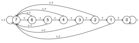
(The edges denote the possible transitions, the labels are the probabilities of a given step.)

Another way to summarise the Markov chain is via its transition matrix:

What does this mean? If you take its k’th column (indexing from 0), that is the distribution you get after one step from state k. Taking the k’th column of a matrix is the same as multiplying it by the k’th unit vector. (Vector that’s 0 everywhere and 1 in the k’th place.) The nice thing is that it works for distributions as well: if you multiply it by a vector that denotes a distribution over the states, the result will be the distribution after the next step. This means that the N’th power of this matrix is the distribution after n steps. If you take its last column, that’s the distribution of your N’th step starting from 7, and if you take this vector’s first (zeroth) value, that’s the probability of you having failed.

Now, I did not find a nice easy way to calculate that, you’d have to do the actual matrix multiplication. However, this is computationally a lot cheaper. (For the previous recursive algorithm, you need log(N) multiplications to calculate the final result. With the matrix multiplication method, you need log N matrix multiplications, each of which consists of 4096 regular multiplications.)

Of course the solution is the same (except that I calculated the probability of failure outright, so my number is 1 minus @wobster109​‘s number), and with a number as low as 15000 it won’t make a difference (I believe the recursive algorithm might even be faster), but for larger N’s, the difference grows. (Although I’d be remiss if I didn’t mention that for this algorithm, you use more space: you need to store all log(N) matrices, while the above algorithm only needs to store 7 numbers, regardless of N.)

I generally consider myself a fairly grounded person, but when I manage to biff a dice roll with an 85% chance of success seven times in a row, I can't help but start to wonder.

[pineappleicedtea]

Wednesday 4 January 2023

Today I got ready for my Berlin trip. I have to wake up at about 5~6am, which I am not looking forward to, considering the fact it's already gone past midnight as I write this.

I spent an hour today on the bus trying to figure out why the transition matrix of a Markov chain always has one as an eigenvalue; moments after getting off I realised the answer was embarrassingly simple. I was simultaneously watching the episode of Breaking Bad season 2 where Hank meets the Tortuga guy and the episode after that where you meet Saul Goodman entitled 'Saul Goodman'.

You guessed it--Tesco meal deal--that's right (I'm imagining Vine boom sound effects in my head). I had some leftover udon so my friend combined it with some instant ramen and squid to make us dinner today. This is the same friend whom I bought the salmon off yesterday (I feel compelled to mention that they cooked yesterday's salmon for me too...just the salmon because I was afraid I'd cook it wrong somehow). The squid was awesome; the noodles were a bit plain but it wasn't something a bit of spice couldn't fix.

[deepyanti]

Top tech terms for 2022

Sparse matrix Sparse matrices are very useful for computing large-scale applications that dense matrices that are just very difficult to handle .

Markov chain A Markov chain is a mathematical system that experiences transitions from one state to another according to certain probabilistic rules.

Artificial Intelligence AI is a machine, simulating human intelligence, to trigger problem-solving and learning, and also mimic functions associated with the human mind.

Voice Recognition System Voice recognition is the process of inputting a voice chat into a computer program. It is important for providing a seamless hands-free experience.

Dimensionality reduction Dimensionality reduction is reducing the number of input variables in the training data for ML models,thus helping the models perform more effectively

Probability density function Probability density function is a function whose value at any given point in the sample space can be interpreted relative to the random variable.

Data parallelism Data parallelism refers to spreading tasks across several processors or nodes which perform operations parallelly in parallel computing environments.

Algorithmic bias Algorithmic bias refers to the lack of fairness in the outputs generated by an algorithm. These may include age discrimination, gender and racial bias

Customer Feedback Customer feedback is the information provided by the customer, on the overall experience with the brand to check their satisfaction level.

Multi-Channel Support Multi-channel support is a set of two or more individual support channels that a business utilizes to communicate with its end-users.

Algorithms In computer programming, an algorithm is a series of well-defined instructions to solve a particular problem or produce the desired results using data

Communications Platform as a Service (CPaaS) Communications platform as a service or CPaaS, is a cloud-based platform that helps developers to implement real-time communication features.

Customer Touchpoint Customer touch points are essential points of interactions between businesses and customers that occur during the customer’s journey.

WhatsApp Broadcast WhatsApp Broadcast allows individuals or businesses to send messages to a list of recipients or contacts in one go without creating a group.

Natural language understanding Natural language understanding a subfield of Natural Language Processing (NLP) and focuses on converting human language into machine-readable formats.

Radial basis function network In mathematical modeling, a radial basis function network is an artificial neural network that uses radial basis functions as activation functions.

DBSCAN Density-Based Spatial Clustering of Applications with Noise is a popular learning method utilized in model building and machine learning algorithms.

Behavior informatics Behavior informatics (BI) is the informatics of behaviors so as to obtain behavior intelligence and behavior insights and science.

Regression Analysis Regression analysis is a set of statistical processes for estimating the relationships between a dependent variable & one or more independent variable

Customer Personas A customer persona is a semi-fictional character of your ideal customer, based on the data you’ve collected from user research & web analytics.

Perceptron Perceptron is an algorithm used for supervised learning of binary classifiers. It classifies data in 2 sections & is called a linear binary classifier

Normalization Normalization organizes attributes and relations of a database to ensure that database integrity constraints properly enforce their dependencies.

[randomforst]

Social Networks: Theory and Implementation Series Part1

Hi, WTF I have my 3 last exams of my Master’s Degree in AI and one of them is about Social Networks: Theory and Implementation. Or a cooler way to call it: How to hack Tinder(?)

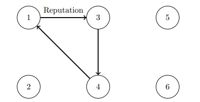
Anyway you can understand how pages rank other webpages, profiles, songs, etc. Lets say NODES.

We can say that the node or page with more recommendations, i.e. better reputation, should be more important than another one with fewer recommendations. If the page with a high reputation recommends another one, then the reputation of this other one will increase and so on. This last page can recommend the first one forming a circularity.

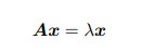
The circularity can be undone with the idea of eigenvalues in which the highest ranked nodes have the highest number of inputs because they are better connected.

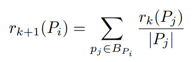
The original PageRank formula

The creators of this idea summarised the PageRank equation of a page (let's call it r(Pi) as the sum of all PageRanks pointing to PiSo we get the following formula, quite simple (for the moment xd).

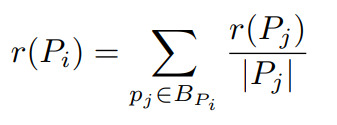
Bp refers to the set of pages pointing in Pi

But the problem is that the value of r(Pj) is unknown and therefore an iterative formula was developed in which r of k+1 (Pj) is taken into account, which corresponds to the PageRank of the page in iteration k+1.

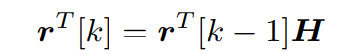
And this equation is usually presented as a Matrix  H. The following graph is represented by the example matrix:

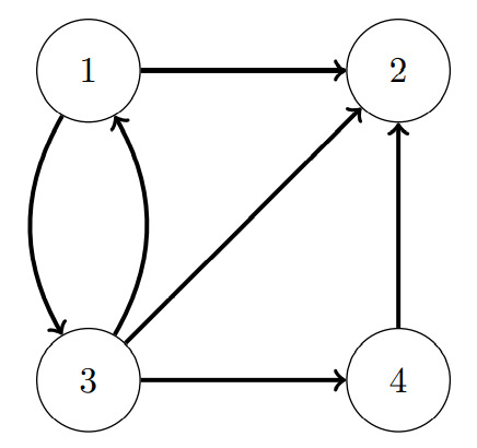
And therefore, we can define the equation as: 

Markov Chains and the Random Surfer

Markov Chains used here. They are a stochastic process where the probability of an event depends exclusively to the previous event. But the main problem is the called dangling node. The dangling nodes are the nodes in network that have no connections and therefore, creates 0 rows. The non-danglin nodes create stochastic rows so the Matrix H is called sub-stochastic matrix.

The Random Surfer is the way the creators of PageRank describe the dangling problem. Where there is a surfer who is going from a page of the internet, and when we arrives to a webpage, he randomly chooses a hyperling and arrives to a new page. He do this process indefinitely. Finally the surfer gets caught when he enters to a dangling node, and as we know the Internet is full of dangling node pages, such as images or pdf files.

To solve this problem, matrix S is defined. A matrix that substitutes H matrix called stochastic matrix S. This matrix S substitutes all the zero rows by 1/n where n is the dimension of the matrix. This guarantees that S is stochastic and then it is the transition probability matrix for the Markov chain.

Finally the S matrix cannot guarantee the convergence result desired. It does not take into account Isolated Convergences and therefore, It is not a primitive matrix.

[clunce]

HW Assignment Review the application article attached to this assignment Complet

HW Assignment Review the application article attached to this assignment Complet

HW Assignment Review the application article attached to this assignment Complete the 2 tasks Task 1 Review the 6 pages from the application article associated with this assignment •The full article, if interested, can be found here http://www.med.mcgill.ca/epidemiology/courses/EPIB654/Summer2010/Modeling/Markov%20modles%20in%20med%20dec%20making.pdf 1. Use R to generate the transition matrix…

[distpubindia]

Decision Science MCQ Set 3

Decision Science MCQ Set 3

QN1. In Markov analysis, state probabilities musta. Sum to oneb. Be less than onec. Be greater than oned. None of the above QN2. State transition probabilities in the Markov chain shoulda. Sum to 1b. Be less than 1c. Be greater than 1d. None of the above QN3. If a matrix of transition probability is of the order n*n, then the number of equilibrium equations would bea. nb. n-1c. n+1d. None of…

[pius2017]

Let {Xt,t 0,1,2,...J be a Markov chain with three states (S 1,2,3]), initial distribution (0.2,0.3,0.5) and transition probability matrix P0.5 0.3 0.2 0 0.8 0.2 (a) Find P(Xt+2 1, Xt+1-2Xt 3)

Let {Xt,t 0,1,2,…J be a Markov chain with three states (S 1,2,3]), initial distribution (0.2,0.3,0.5) and transition probability matrix P0.5 0.3 0.2 0 0.8 0.2 (a) Find P(Xt+2 1, Xt+1-2Xt 3)

1. Let {Xt,t 0,1,2,…J be a Markov chain with three states (S 1,2,3]), initial distribution (0.2,0.3,0.5) and transition probability matrix P0.5 0.3 0.2 0 0.8 0.2 (a) Find P(Xt+2 1, Xt+1-2Xt 3) (b) Find the two step transition probability matrix P2) and specifically (e) Find P(X2-1 (d) Find EXi.

[1handedecon]

Dynamic clustering of multivariate panel data

We propose a dynamic clustering model for uncovering latent time-varying group structures in multivariate panel data. The model is dynamic in three ways. First, the cluster location and scale matrices are time-varying to track gradual changes in cluster characteristics over time. Second, all units can transition between clusters based on a Hidden Markov model (HMM). Finally, the HMM’s transition matrix can depend on lagged time-varying cluster distances as well as economic covariates. Monte Carlo experiments suggest that the units can be classified reliably in a variety of challenging settings. Incorporating dynamics in the cluster composition proves empirically important in an a study of 299 European banks between 2008Q1 and 2018Q2. We find that approximately 3% of banks transition per quarter on average. Transition probabilities are in part explained by differences in bank profitability, suggesting that low interest rates can lead to long-lasting changes in financial industry structure. from ECB - European Central Bank https://ift.tt/2WyLJRW via IFTTT

[dreamassignmenthelp]

Influence of State Transition Matrix in Control System Engineering

What is state transition matrix in control system?

In a classical system, there is an involvement of plants say G of s, we are applying input and we are getting the output. So input is applied. At t equals 0, we are expecting that the output at certain time interval output says at t equals 10 secs. Now, this is the step input and now is the output. So here output we have got at t equals 10 secs. But in the state of the state-space system along with this output, there are states which are the important parameter in the system, that has been traveled that is from t equals to 0 to t equals to f, the state has been transferred. So this transferring of the states tell about the state transition matrix. Now, how you define the state transition matrix. If you want to know What is state transition matrix in control system, you can send us an email.

It is defined as the transition of states from the initial time t =0 to any time “t” or final time (tf) when the inputs are zero., that is this trans-state transition matrix has not concerned with any type of input. It is concerned with some initial state that is t =0 to tf.

The Significance of The State Transition Matrix

· It is defined as the solution of the linear homogeneous state equation. We have seen last time, the X =AX, X(t)= eAtX (0), this eAtis called the state transition matrix and this is a homogeneous state equations. .

· It is the response due to initial vector x(0).

Here if you consider X dot = AX +BU, X(t)= eAtX= 0 to t, some values will get here coefficient will get and we have written d of t. so in this particular case, this is u of t. it has taken care of X naught only, whereas if you take this part , this portion that is a forced portion, forced part in this particular part there is no involvement of X naught. So, therefore we are saying

· It is dependent on the initial state vector and not the input. Here in this forced part there is no initial state has been involved, but as far as we are discussing with the state transition matrix it is concern with the zero ,

· It is called the zero input response since the input is zero. It is called the free response

· It is called as the free response of the system, since the response is excited by the initial conditions only. You can get the significance of the state transition matrix.

Properties of state transition matrix

A matrix is often referred to A rectangular arrangement of numbers in rows and columns..Now in Engineering, Control theory refers to the control of continuously operating dynamical systems in engineered processes and machines. The state-transition matrix is a matrix whose product with the state vector x at the time t0 gives x at a time t, where t0denotes the initial time. State transition matrix helps to find the general solution of linear dynamical systems. It is represented by Φ. It plays an important part of two conditions that is the zero input and the zero state solutions of systems represented in state space.

1.It has continuous derivatives.

2. It is continuous.

3. It cannot be singular. Φ-1(t, 𝜏) = Φ(𝜏, t)

Φ-1 (t, 𝜏) Φ(t, 𝜏) = I. I is the identity matrix.

4. Φ(t, t) = I ∀ t.

5. Φ (t2,t1) Φ(t1, t0) = Φ(t2, t0) ∀ t0≤ t1≤ t2

6. Φ(t, 𝜏) = U(t) U-1(𝜏).

U(t) is an n×n matrix. It is the fundamental solution matrix that satisfies the following equation with initial condition U(t0) = I.

U˙(t)=A(t)U(t)\dot{U}(t) = A(t) U(t)U˙(t)=A(t)U(t)

7. It also satisfies the following differential equation with initial conditions Φ(t0, t0) = I

∂ϕ(t,t0)∂t=A(t)ϕ(t,t0)\frac{\partial \phi(t, t_0)}{\partial t} = A(t) \phi(t, t_0)∂t∂ϕ(t,t0​)​=A(t)ϕ(t,t0​)

8. x(t) = Φ(t, 𝜏) x(𝜏)

9. The inverse of this gives the same as that of the state transition matrix , replacing ‘t’ by ‘-t’. Φ-1(t) = Φ(-t).

10. Φ(t1 + t2) = Φ(t1)Φ(t2) .If t = t1 + t2, the resulting state transition matrix is equal to the multiplication of the two state transition matrices at t = t1and t = t2.

Consider a general state equation, X˙=AX(t) , (eq 1) where X is state matrix, A is system matrix. thus its general homogeneous answer are often given as series of t [from ODE], X(t)=bo+b1t+b1t2+….+bktk+ …, (eq 2) So (eq 1) are often written as: b1+2b2t+3b3t2=A(bo+b1t+b1t2+….) Comparing the constantwe tend toget, b1=Abo;b2=12A2bo;bk=1k!Akbo We see, on golf shot t=0 in (eq 2), X(0)=bo=initial condition So X(t) are often re written as X(t)=[I+At+12A2t2+…+1k!Ak+…]n x n matrix X (0) i.e, X(t) = eAt(an operator on initial condition) X(0) (initial condition) We can create following conclusion: State transition matrix Φ(t) = eAt, is infinite series that converges for all A and for all finite price of t. Φ(t) operates on state vector initial condition to urge answer for all t≥0. State transition matrix contain all the knowledge concerning the free response of system once input is zero, or, the system is worked up by initial conditions solely. So, state transition matrix Φ(t) , defines transition of states from initial time t to any time t once input is zero. We tend to get the truncated series of finite term. Best helpful properties of state transition matrix Φ(t) is: Φ(t2−t1)Φ(t1−t0) = eA(t2−t1)eA(t1−to)= eA(t2−to) = Φ(t2−to). This property is vital, since it implies that a state transition method are often divided into range of serial transitions. You can get a clear idea of state transition matrix properties.

Takeaways

State transition Matrix is thus a sq. likelihood matrix whose columns total to one. It describes the demographic population amendment from year to year or the amendment of the market costs from year to year. It typically is delineated as a Markov process. We provide control systems engineering online tutors for helping engineering students to complete their dream assignments within the deadline. Reach us soon and take the best expert help.

[tilde-he]

Epistemic status: full of question marks. exploratory? dreaming big, perhaps of things impossibly big. Right, so,

I saw a couple papers (which I didn’t entirely understand, but seemed neat) about different theories of probabilities which use infinitesimals in the probability values (one of which was this one (<-- not sure that link will actually work. Let me know if it doesn’t?), and the other one I can’t find right now but was similar, used the same system I think, though it also dealt with uniform probability distributions over the rational interval from 0 to 1) and they built their stuff using nonstandard models of the natural numbers, where, if I’m understanding correctly, they got some nonstandard integer to represent “how many standard natural numbers there are”, or something like that. Also, they defined limits in a way that was like, as some variable ranging over the finite subsets of some infinite set gets larger in the sense of subsets, then the value “approaches” the limit in some sense, and I think this was in a way connected to ultrafilters and the nonstandard models of arithmetic they were using. I did not actually follow quite how they were defining these limits.

(haha I still don’t actually understand ultrafilters in such a way that I remember quite what they are without looking it up.)

Intro to the Idea:

So, I was wondering if maybe it might work out in an interesting way to apply this theory of probability to markov chains when, say, all of the states are in one (aperiodic) class, and are recurrent, but none of them are positive recurrent (or, alternatively, some of them could be positive recurrent, but almost all of them would not be), in order to get a stationary distribution with appropriate infinitesimals?

Feasibility of the Idea:

It seems to me like that should be possible to work out, because I think the system the authors of those papers define is well-defined and such, and can probably handle this situation fine? Yeah, uh, it does handle infinite sequences of coin tosses, and assigns positive (infinitesimal) probability to the event “all of them land heads” (and also a different infinitesimal probability which is twice as large to the event “all of them after the first one land heads (and the first one either lands heads or tails)” ), and I think that suggests that it can probably handle events like, uh, “in a random walk on Z where left and right have probability 1/2 each, the proportion(?) of the steps which are in the same state as the initial state, is [????what-sort-of-thing-goes-here????]”, because they could just take all the possible cases where the proportion(?) is  [????what-sort-of-thing-goes-here????], and each of these cases would correspond to a particular infinite sequence of coin tosses, which each have the same infinitesimal probability, and then those could just be “added up” using the limit thing they defined, and that should end up with the probability of the proportion(?) being [????what-sort-of-thing-goes-here????].

Building Up the Idea:

So, if that all ends up working out with normal markov chains, then the next step I see would be to attempt to apply it to markov chains where the matrix of transition probabilities itself has values which are infinitesimal, or have infinitesimal components, and, again, trying to get stationary distributions out of those (which would again have infinitesimal values for some of the states). Specifically, one case that I think would be good to look at would be the case where a number is picked uniformly at random from the natural numbers and combined with the current state in order to get the next state (or, perhaps, a pair of natural numbers). Or from some other countably infinite set. So, then (if that all worked out), you could talk about stuff like a stationary distribution of a uniform random walk on Z^N and stuff like that.

The Idea:

If all that stuff works out, then, take this markov chain: State space: S∞ , the symmetric group on N, or alternatively the normal subgroup of S∞  comprised of its elements which fix all but at most finitely many of the elements of N. Initial state (if relevant) : The identity permutation. State transitions: Pick two natural numbers uniformly at random from N, and apply the transposition of those two natural numbers to the current state. Desired outcome: A uniform probability distribution on S∞ (or on the normal subgroup of it of finite permutations)!!!  (likely with infinitesimal components in the probabilities, but one can take the standard part of these probabilities, and at least under conditioning maybe these would even be positive.)

Issues and Limitations:

Even if this all works out, I’m not sure it would really give me quite what I want. Notably, in the systems described in the papers I read-but-did-not-fully-understand, for some events, the standard parts of the probabilities of some events depended on the ultrafilter chosen.

Also, if every (or even “most”) of the permutations had an infinitesimal probability (i.e. a nonzero probability with standard part 0) in the stationary distribution, that probably wouldn’t really do what I want it to do. Or, really, no, that’s not quite the problem. If the exact permutations had infinitesimal probability, that could be fine, but I would hope that the events of the form “the selected permutation begins with the finite prefix σ” would all have probabilities with positive standard part.

But, it seems plausible, even likely, that if this all worked, that for any natural number n, that the probability that a permutation selected from such a stationary distribution would send 1 to a number less than n, would be infinitesimal. (not a particular infinitesimal. The specific infinitesimal would depend on n, and would increase as n increased, but would remain infinitesimal for any finite n).

This is undesirable! I wouldn’t be able to sample prefixes to this in the same way that I can sample prefixes to infinite sequences of coin tosses.

(Alternatively, it might turn out that the standard part of the probability that the selected permutation matches the identity permutation for the first m integers is 1, as a result the probability that a transposition include one of the first m integers being infinitesimal, which might be less unfortunate, but still seems bad? I’m less certain that this outcome would be undesirable.)

I think that, what I really want, would require having a probability distribution on N which, while not uniform, would be the “most natural” probability distribution on N, in the same way that the uniform distribution on {1,2,3,4} appears to be the “most natural” probability distribution on {1,2,3,4}, when one has no additional information, and also that said distribution on N would have positive (standard parts of) probabilities for each natural number.

To have this would require both finding such a distribution, and also showing that that distribution really is the “most natural” probability distribution on N. Demonstrating that such a distribution really is the “most natural” seems likely to be rather difficult, especially given that I am uncertain of exactly what I mean when I say “most natural”.

...

If I should have put a read-more in here, sorry. I can edit the post to put one in if you tell me to. edit: forgot to put in the “σ” . did that now.