#OrderedDict() collection

[pythontipsnadtricks]

Built-in Modules in Python

Built-in modules in Python (learn python online) are pre-existing libraries that provide a wide range of functionalities to streamline and simplify various programming tasks. These modules are available as part of the standard Python library and cover a diverse array of areas, from mathematical calculations to working with files and managing dates. Here are some key built-in modules in Python:

math: This module offers mathematical functions, such as trigonometric, logarithmic, and arithmetic operations, providing access to mathematical constants like pi and e.

datetime: The datetime module allows manipulation and formatting of dates and times. It includes classes for working with dates, times, time intervals, and timezones.

random: The random module enables the generation of random numbers, providing functions for generating random integers, floating-point numbers, and random selections from sequences.

os: The os module offers a wide range of operating system-related functionalities. It provides functions for interacting with the file system, working with directories, and executing system commands.

sys: The sys module provides access to Python interpreter variables and functions, allowing interaction with the runtime environment. It's commonly used for handling command-line arguments and controlling the Python interpreter.

re: The re module is used for regular expression operations. It enables pattern matching and manipulation of strings based on specified patterns.

json: The json module facilitates encoding and decoding of JSON (JavaScript Object Notation) data, which is widely used for data interchange between applications.

collections: The collections module provides additional data structures beyond the built-in ones. It includes specialized container data types like OrderedDict, defaultdict, and namedtuple.

math: The math module contains mathematical functions and constants for more advanced calculations, including trigonometric, logarithmic, and exponential operations.

time: The time module provides functions for working with time-related tasks, including measuring execution times, setting timeouts, and creating timestamps.

csv: The csv module offers tools for reading and writing CSV (Comma-Separated Values) files, which are commonly used for tabular data storage.

heapq: The heapq module provides heap-related functions, allowing for the implementation of priority queues and heap-based algorithms.

These built-in modules save time and effort by providing pre-built solutions for common programming tasks. By utilizing these modules, developers can avoid reinventing the wheel and focus on creating more efficient and feature-rich applications.

[webbazaar0101]

OrderedDict() collection:

OrderedDict() collection: Dictionary subclass that remembers the entry order. The OrderedDict() collection is similar to a dictionary object where keys maintain the order of insertion, whereas in the normal dictionary the order is arbitrary......

Dictionary subclass that remembers the entry order. The OrderedDict() collection is similar to a dictionary object where keys maintain the order of insertion, whereas in the normal dictionary the order is arbitrary. If we try to insert the key again, the previous value will be overwritten for that key. Syntax: collections.OrderDict() Example: import…

[iwebscrapingblogs]

How To Scrape Expedia Using Python And LXML?

When done manually, gathering travel data for planes is a massive undertaking. There are various possible combinations of airports, routes, times, and costs, all of which are always changing. Ticket rates fluctuate on a daily (or even hourly) basis, and there are numerous flights available each day. Web scraping is one method for keeping track of this information. In this Blog, we'll scrape Expedia , a popular vacation booking site, to get flight information. The flight schedules and pricing for a sender and the receiver pair will be extracted by our scraper.

Data Fields that will be extracted:

Arrival Airport

Arrival Time

Departure Airport

Departure Time

Flight Name

Flight Duration

Ticket Price

No. Of Stops

Airline

Below shown is the screenshot of the data fields that we will be extracting:

Scraping Code:

1. Create the URL of the search results from Expedia for instance, we will check the available flights listed from New York to Miami:

https://www.expedia.com/Flights-Search?trip=oneway&leg1=from:New%20York,%20NY%20(NYC-All%20Airports),to:Miami,%20Florida,departure:04/01/2017TANYT&passengers=children:0,adults:1,seniors:0,infantinlap:Y&mode=search

2. Using Python Requests, download the HTML of the search result page.

3. Parse the webpage with LXML — LXML uses Xpaths to browse the HTML Tree Structure. The XPaths for the details we require in the code have already been defined.

4. Save the information in a JSON file. You can change this later to write to a database.

Requirements

We'll need several libraries for obtaining and parsing HTML for this Python 3 web scraping tutorial. The requirements for the package are shown below.

Install Python 3 and Pip

Install Packages

The code is explanatory

You can check the code from the link here.

Executing the Expedia Scraper

Let's say the script's name is expedia.py. In a command prompt or terminal, input the script name followed by a -h.

usage: expedia.py [-h] source destination date positional arguments: source            Source airport code destination       Destination airport code date              MM/DD/YYYY optional arguments: -h, --help show this help message and exit

The input and output arguments are the airline codes for the source and destination airports, respectively. The date parameter must be in the form MM/DD/YYYY

For example, to get flights from New York to Miami, we would use the following arguments:

python3 expedia.py nyc mia 04/01/2017

The nyc-mia-flight-results.json file will be created as a result of this. json, which will be saved in the same directory as the script.

This is what the output file will look like:

{ "arrival": "Miami Intl., Miami", "timings": [ { "arrival_airport": "Miami, FL (MIA-Miami Intl.)", "arrival_time": "12:19a", "departure_airport": "New York, NY (LGA-LaGuardia)", "departure_time": "9:00p" } ], "airline": "American Airlines", "flight duration": "1 days 3 hours 19 minutes", "plane code": "738", "plane": "Boeing 737-800", "departure": "LaGuardia, New York", "stops": "Nonstop", "ticket price": "1144.21" }, { "arrival": "Miami Intl., Miami", "timings": [ { "arrival_airport": "St. Louis, MO (STL-Lambert-St. Louis Intl.)", "arrival_time": "11:15a", "departure_airport": "New York, NY (LGA-LaGuardia)", "departure_time": "9:11a" }, { "arrival_airport": "Miami, FL (MIA-Miami Intl.)", "arrival_time": "8:44p", "departure_airport": "St. Louis, MO (STL-Lambert-St. Louis Intl.)", "departure_time": "4:54p" } ], "airline": "Republic Airlines As American Eagle", "flight duration": "0 days 11 hours 33 minutes", "plane code": "E75", "plane": "Embraer 175", "departure": "LaGuardia, New York", "stops": "1 Stop", "ticket price": "2028.40" },

You can download the code at:

import json import requests from lxml import html from collections import OrderedDict import argparse def parse(source,destination,date): for i in range(5): try: url = "https://www.expedia.com/Flights-Search?trip=oneway&leg1=from:{0},to:{1},departure:{2}TANYT&passengers=adults:1,children:0,seniors:0,infantinlap:Y&options=cabinclass%3Aeconomy&mode=search&origref=www.expedia.com".format(source,destination,date) headers = {'User-Agent': 'Mozilla/5.0 (Windows NT 10.0; Win64; x64) AppleWebKit/537.36 (KHTML, like Gecko) Chrome/70.0.3538.77 Safari/537.36'} response = requests.get(url, headers=headers, verify=False) parser = html.fromstring(response.text) json_data_xpath = parser.xpath("//script[@id='cachedResultsJson']//text()") raw_json =json.loads(json_data_xpath[0] if json_data_xpath else '') flight_data = json.loads(raw_json["content"]) flight_info  = OrderedDict() lists=[] for i in flight_data['legs'].keys(): total_distance =  flight_data['legs'][i].get("formattedDistance",'') exact_price = flight_data['legs'][i].get('price',{}).get('totalPriceAsDecimal','') departure_location_airport = flight_data['legs'][i].get('departureLocation',{}).get('airportLongName','') departure_location_city = flight_data['legs'][i].get('departureLocation',{}).get('airportCity','') departure_location_airport_code = flight_data['legs'][i].get('departureLocation',{}).get('airportCode','') arrival_location_airport = flight_data['legs'][i].get('arrivalLocation',{}).get('airportLongName','') arrival_location_airport_code = flight_data['legs'][i].get('arrivalLocation',{}).get('airportCode','') arrival_location_city = flight_data['legs'][i].get('arrivalLocation',{}).get('airportCity','') airline_name = flight_data['legs'][i].get('carrierSummary',{}).get('airlineName','') no_of_stops = flight_data['legs'][i].get("stops","") flight_duration = flight_data['legs'][i].get('duration',{}) flight_hour = flight_duration.get('hours','') flight_minutes = flight_duration.get('minutes','') flight_days = flight_duration.get('numOfDays','') if no_of_stops==0:    stop = "Nonstop" else:    stop = str(no_of_stops)+' Stop' total_flight_duration = "{0} days {1} hours {2} minutes".format(flight_days,flight_hour,flight_minutes) departure = departure_location_airport+", "+departure_location_city arrival = arrival_location_airport+", "+arrival_location_city carrier = flight_data['legs'][i].get('timeline',[])[0].get('carrier',{}) plane = carrier.get('plane','') plane_code = carrier.get('planeCode','') formatted_price = "{0:.2f}".format(exact_price) if not airline_name:    airline_name = carrier.get('operatedBy','') timings = [] for timeline in  flight_data['legs'][i].get('timeline',{}):    if 'departureAirport' in timeline.keys():        departure_airport = timeline['departureAirport'].get('longName','')        departure_time = timeline['departureTime'].get('time','')        arrival_airport = timeline.get('arrivalAirport',{}).get('longName','')        arrival_time = timeline.get('arrivalTime',{}).get('time','')        flight_timing = {                            'departure_airport':departure_airport,                            'departure_time':departure_time,                            'arrival_airport':arrival_airport,                            'arrival_time':arrival_time        }        timings.append(flight_timing) flight_info={'stops':stop,    'ticket price':formatted_price,    'departure':departure,    'arrival':arrival,    'flight duration':total_flight_duration,    'airline':airline_name,    'plane':plane,    'timings':timings,    'plane code':plane_code } lists.append(flight_info)    sortedlist = sorted(lists, key=lambda k: k['ticket price'],reverse=False)    return sortedlist except ValueError:    print ("Rerying...")     return {"error":"failed to process the page",} if __name__=="__main__": argparser = argparse.ArgumentParser() argparser.add_argument('source',help = 'Source airport code') argparser.add_argument('destination',help = 'Destination airport code') argparser.add_argument('date',help = 'MM/DD/YYYY') args = argparser.parse_args() source = args.source destination = args.destination date = args.date print ("Fetching flight details") scraped_data = parse(source,destination,date) print ("Writing data to output file") with open('%s-%s-flight-results.json'%(source,destination),'w') as fp: json.dump(scraped_data,fp,indent = 4)

Unless the page structure changes dramatically, this scraper should be able to retrieve most of the flight details present on Expedia. This scraper is probably not going to work for you if you want to scrape the details of thousands of pages at very short intervals.

Contact iWeb Scraping for extracting Expedia using Python and LXML or ask for a free quote!

https://www.iwebscraping.com/how-to-scrape-expedia-using-python-and-lxml.php

[goodwallfree]

Collections.OrderedDict()

collections.OrderedDict

An OrderedDict is a dictionary that remembers the order of the keys that were inserted first. If a new entry overwrites an existing entry, the original insertion position is left unchanged.

Example

Code :>>> from collections import OrderedDict >>> >>> ordinary_dictionary = {} >>> ordinary_dictionary['a'] = 1 >>> ordinary_dictionary['b'] = 2 >>> ordinary_dictionary['c'] = 3 >>> ordinary_dictionary['d'] = 4 >>> ordinary_dictionary['e'] = 5 >>> >>> print ordinary_dictionary {'a': 1, 'c': 3, 'b': 2, 'e': 5, 'd': 4} >>> >>> ordered_dictionary = OrderedDict() >>> ordered_dictionary['a'] = 1 >>> ordered_dictionary['b'] = 2 >>> ordered_dictionary['c'] = 3 >>> ordered_dictionary['d'] = 4 >>> ordered_dictionary['e'] = 5 >>> >>> print ordered_dictionary OrderedDict([('a', 1), ('b', 2), ('c', 3), ('d', 4), ('e', 5)])

Task :

You are the manager of a supermarket. You have a list of N items together with their prices that consumers bought on a particular day. Your task is to print each item_name and net_price in order of its first occurrence.

item_name = Name of the item. net_price = Quantity of the item sold multiplied by the price of each item.

Input Format :

The first line contains the number of items, N.

The next N lines contains the item’s name and price, separated by a space.

Constraints :

0 < N <= 100

Output Format :

Print the item_name and net_price in order of its first occurrence.

Sample Input :

9 BANANA FRIES 12 POTATO CHIPS 30 APPLE JUICE 10 CANDY 5 APPLE JUICE 10 CANDY 5 CANDY 5 CANDY 5 POTATO CHIPS 30

Sample Output :

BANANA FRIES 12 POTATO CHIPS 60 APPLE JUICE 20 CANDY 20

Explanation :

BANANA FRIES: Quantity bought: 1, Price: 12 Net Price: 12 POTATO CHIPS: Quantity bought: 2, Price: 30 Net Price: APPLE JUICE: Quantity bought: 2, Price: 10 Net Price: 20 CANDY: Quantity bought: 4, Price: 5

Net Price:20

Solution

from collections import*; N = int(input()); d = OrderedDict(); for i in range(N): item = input().split() itemPrice = int(item[-1]) itemName = " ".join(item[:-1]) if(d.get(itemName)): d[itemName] += itemPrice else: d[itemName] = itemPrice for i in d.keys(): print(i, d[i])

Result

[courseradmv]

DVM Week 3 Assignment Code

import pandas

import numpy

from collections import OrderedDict

from tabulate import tabulate, tabulate_formats

Step 2: Read the specific columns of the dataset and rename the columns

data = pandas.read_csv(‘CodebookGap.csv’, low_memory=False, skip_blank_lines=True, usecols=[‘country’,’incomeperperson’, ‘alcconsumption’, ‘lifeexpectancy’] )

data.columns=[‘country’, ‘income’, ‘alcohol’, ‘life’]

data.info()

Step 3: convert arguments to a numeric types from .csv files

for dt in (‘income’,’alcohol’,’life’) :

data[dt] = pandas.to_numeric(data[dt], errors=’coerce’)

data.info()

nullLabels =data[data.country.isnull() | data.income.isnull() | data.alcohol.isnull() | data.life.isnull()]

print(nullLabels)

Step 4: Drop the missing data rows

data = data.dropna(axis=0, how=’any’)

print (data.info())

Step 5: Display absolute and relative frequency

c2 = data[‘income’].value_counts(sort=False)

p2 = data[‘income’].value_counts(sort=False, normalize=True)

c3 = data[‘alcohol’].value_counts(sort=False)

p3 = data[‘alcohol’].value_counts(sort=False, normalize=True)

c4 = data[‘life’].value_counts(sort=False)

p4 = data[‘life’].value_counts(sort=False, normalize=True)

print(“**”)

print(“Absolute Frequency*”)

print(“Income Per Person:”)

print(“Income Freq”)

print(c2)

print(“Alcohol Consumption:”)

print(“Alcohol Freq”)

print(c3)

print(“Life Expecectancy:”)

print(“Life Freq”)

print(c4)

print(“**”)

print(“Relative Frequency*”)

print(“Income Per Person:”)

print(“Income Freq”)

print(p2)

print(“Alcohol Consumption:”)

print(“Alcohol Freq”)

print(p3)

print(“Life Expecectancy:”)

print(“Life Freq”)

print(p4)

Step 6: Make groups in variables to understand such research question

minMax = OrderedDict()

dict1 = OrderedDict()

dict1[‘min’] = data.life.min()

dict1[‘max’] = data.life.max()

minMax[‘life’] = dict1

dict2 = OrderedDict()

dict2[‘min’] = data.income.min()

dict2[‘max’] = data.income.max()

minMax[‘income’] = dict2

dict3 = OrderedDict()

dict3[‘min’] = data.alcohol.min()

dict3[‘max’] = data.alcohol.max()

minMax[‘alcohol’] = dict3

df = pandas.DataFrame([minMax[‘income’],minMax[‘life’],minMax[‘alcohol’]], index = [‘Income’,’Life’,’Alcohol’])

print (df.sort_index(axis=1, ascending=False))

dummyData = data.copy()

Maps

income_map = {1: ‘>=100 <5k’, 2: ‘>=5k <10k’, 3: ‘>=10k <20k’,

4: ‘>=20K < 30K’, 5: ‘>=30K <40K’, 6: ‘>=40K <50K’ }

life_map = {1: ‘>=40 <50’, 2: ‘>=50 <60’, 3: ‘>=60 <70’, 4: ‘>=70 <80’, 5: ‘>=80 <90’}

alcohol_map = {1: ‘>=0.5 <5’, 2: ‘>=5 <10’, 3: ‘>=10 <15’, 4: ‘>=15 <20’, 5: ‘>=20 <25’}

dummyData[‘income’] = pandas.cut(data.income,[100,5000,10000,20000,30000,40000,50000], labels=[‘1’,’2',’3',’4',’5',’6'])

print(dummyData.head(10))

dummyData[‘life’] = pandas.cut(data.life,[40,50,60,70,80,90], labels=[‘1’,’2',’3',’4',’5'])

print(dummyData.head(10))

dummyData[‘alcohol’] = pandas.cut(data.alcohol,[0.5,5,10,15,20,25], labels=[‘1’,’2',’3',’4',’5'])

print (dummyData.head(10))

c2 = dummyData[‘income’].value_counts(sort=False)

p2 = dummyData[‘income’].value_counts(sort=False, normalize=True)

c3 = dummyData[‘alcohol’].value_counts(sort=False)

p3 = dummyData[‘alcohol’].value_counts(sort=False, normalize=True)

c4 = dummyData[‘life’].value_counts(sort=False)

p4 = dummyData[‘life’].value_counts(sort=False, normalize=True)

Step 7: Frequency Distribution of new grouped data

print(“**”)

print(“Absolute Frequency*”)

print(“Income Per Person:”)

print(“Income-Freq”)

print(c2)

print(“Alcohol Consumption:”)

print(“Alcohol-Freq”)

print(c3)

print(“Life Expecectancy:”)

print(“Life-Freq”)

print(c4)

print(“**”)

print(“Relative Frequency*”)

print(“Income Per Person:”)

print(“Income- Freq”)

print(p2)

print(“Alcohol Consumption:”)

print(“Alcohol-Freq”)

print(p3)

print(“Life Expecectancy:”)

print(“Life-Freq”)

print(p4)

import pandas import numpy from collections import OrderedDict import seaborn import matplotlib.pyplot as plt from tabulate import tabulate, tabulate_formats

data = pandas.read_csv('CodebookGap.csv', low_memory=False, skip_blank_lines=True, usecols=['country','incomeperperson', 'alcconsumption', 'lifeexpectancy'])

data.columns=['country', 'income', 'alcohol', 'life'] data.info()

for dt in ('income','alcohol','life') : data[dt] = pandas.to_numeric(data[dt], errors='coerce') data.info()

nullLabels =data[data.country.isnull() | data.income.isnull() | data.alcohol.isnull() | data.life.isnull()] print(nullLabels)

data = data.dropna(axis=0, how='any') print (data.info())

minMax = OrderedDict()

dict1 = OrderedDict() dict1['min'] = data.life.min() dict1['max'] = data.life.max() minMax['life'] = dict1

dict2 = OrderedDict() dict2['min'] = data.income.min() dict2['max'] = data.income.max() minMax['income'] = dict2

dict3 = OrderedDict() dict3['min'] = data.alcohol.min() dict3['max'] = data.alcohol.max() minMax['alcohol'] = dict3

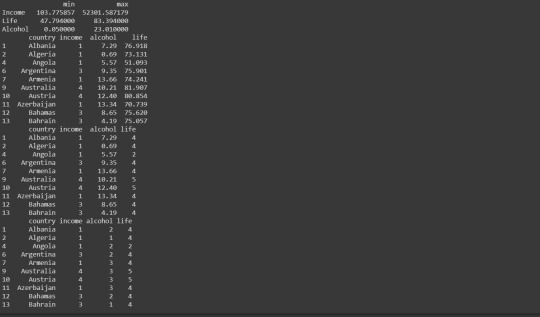
df = pandas.DataFrame([minMax['income'],minMax['life'],minMax['alcohol']], index = ['Income','Life','Alcohol']) print (df.sort_index(axis=1, ascending=False))

dummyData = data.copy() income_map = {1: '>=100 <5k', 2: '>=5k <10k', 3: '>=10k <20k', 4: '>=20K <30K', 5: '>=30K <40K', 6: '>=40K <50K' } life_map = {1: '>=40 <50', 2: '>=50 <60', 3: '>=60 <70', 4: '>=70 <80', 5: '>=80 <90'} alcohol_map = {1: '>=0.5 <5', 2: '>=5 <10', 3: '>=10 <15', 4: '>=15 <20', 5: '>=20 <25'}

dummyData['income'] = pandas.cut(data.income,[100,5000,10000,20000,30000,40000,50000], labels=['1','2','3','4','5','6']) print(dummyData.head(10))

dummyData['life'] = pandas.cut(data.life,[40,50,60,70,80,90], labels=['1','2','3','4','5']) print(dummyData.head(10))

dummyData['alcohol'] = pandas.cut(data.alcohol,[0.5,5,10,15,20,25], labels=['1','2','3','4','5']) print (dummyData.head(10)) min max Income 103.775857 52301.587179 Life 47.794000 83.394000 Alcohol 0.050000 23.010000 country income alcohol life 1 Albania 1 7.29 76.918 2 Algeria 1 0.69 73.131 4 Angola 1 5.57 51.093 6 Argentina 3 9.35 75.901 7 Armenia 1 13.66 74.241 9 Australia 4 10.21 81.907 10 Austria 4 12.40 80.854 11 Azerbaijan 1 13.34 70.739 12 Bahamas 3 8.65 75.620 13 Bahrain 3 4.19 75.057 country income alcohol life 1 Albania 1 7.29 4 2 Algeria 1 0.69 4 4 Angola 1 5.57 2 6 Argentina 3 9.35 4 7 Armenia 1 13.66 4 9 Australia 4 10.21 5 10 Austria 4 12.40 5 11 Azerbaijan 1 13.34 4 12 Bahamas 3 8.65 4 13 Bahrain 3 4.19 4 country income alcohol life 1 Albania 1 2 4 2 Algeria 1 1 4 4 Angola 1 2 2 6 Argentina 3 2 4 7 Armenia 1 3 4 9 Australia 4 3 5 10 Austria 4 3 5 11 Azerbaijan 1 3 4 12 Bahamas 3 2 4 13 Bahrain 3 1 4 c2 = dummyData['income'].value_counts(sort=False) p2 = dummyData['income'].value_counts(sort=False, normalize=True)

c3 = dummyData['alcohol'].value_counts(sort=False) p3 = dummyData['alcohol'].value_counts(sort=False, normalize=True)

c4 = dummyData['life'].value_counts(sort=False) p4 = dummyData['life'].value_counts(sort=False, normalize=True)

print("") print("Absolute Frequency***") print("Income Per Person:") print("Income-Freq") print(c2) print("Alcohol Consumption:") print("Alcohol-Freq") print(c3) print("Life Expecectancy:") print("Life-Freq") print(c4)

print("") print("Relative Frequency***") print("Income Per Person:") print("Income- Freq") print(p2) print("Alcohol Consumption:") print("Alcohol-Freq") print(p3) print("Life Expecectancy:") print("Life-Freq") print(p4)

Absolute Frequency* Income Per Person: Income-Freq 1 110 2 24 3 15 4 12 5 9 6 0 Name: income, dtype: int64 Alcohol Consumption: Alcohol-Freq 1 63 2 56 3 31 4 10 5 1 Name: alcohol, dtype: int64 Life Expecectancy: Life-Freq 1 8 2 28 3 35 4 80 5 20 Name: life, dtype: int64

Relative Frequency* Income Per Person: Income- Freq 1 0.647059 2 0.141176 3 0.088235 4 0.070588 5 0.052941 6 0.000000 Name: income, dtype: float64 Alcohol Consumption: Alcohol-Freq 1 0.391304 2 0.347826 3 0.192547 4 0.062112 5 0.006211 Name: alcohol, dtype: float64 Life Expecectancy: Life-Freq 1 0.046784 2 0.163743 3 0.204678 4 0.467836 5 0.116959 Name: life, dtype: float64

[kushaldube]

Data Management and Visualization - Week 3

Hello, I am Kushal Dube. This Blog is a part of the Data Management and Visualization course by Wesleyan University via Coursera. The assignments in this course are to be submitted in the form of blogs and hence I chose Tumblr as suggested in the course for submitting my assignments. You can read the week 1 blog using these links: Week-1, Week-2.

Here is my codebook:

Research Question:

Is there any relation between life expectancy and alcohol consumption? Is there any relation between Income and alcohol consumption?

Assignment 3:

This assignment contains data management for respective topics. We have to make and implement decisions about data management for the variables. Data Management is a process to store, organize, and maintain data. Security of data is very important to secure the data which is a part of Data Management.

Blog contains:

- Removing missing data rows - Make a group of income, alcohol consumption, and life expectancy - Show frequency distribution before and after grouping

Data Dictionary:

Code:

Step 1: Importing Libraries

#import the libraries import pandas import numpy from collections import OrderedDict

Step 2: Read the specific columns of the dataset and rename the columns

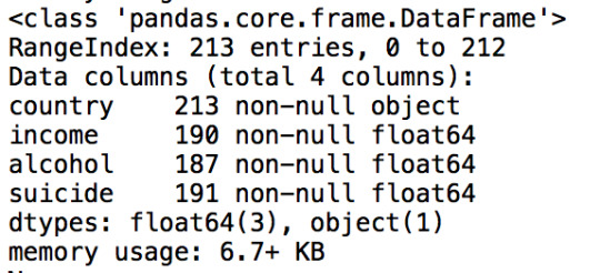
data=pandas.read_csv('gapminder.csv',low_memory=False, skip_blank_lines=True, usecols=['country','incomeperperson','alcconsumption','lifeexpectancy']) data.columns=['country','income','alcohol','life'] ''' #Variable Descriptions alcohol="2008 alcohol consumption per adult (liters,age 15+)" income="2010 Gross Domistic Product per capita in constant 2000 US$" life="2011 life expectancy at birth (years)" ''' data.info()

Output:

<class 'pandas.core.frame.DataFrame'> RangeIndex: 213 entries, 0 to 212 Data columns (total 4 columns): # Column Non-Null Count Dtype --- ------ -------------- ----- 0 country 213 non-null object 1 income 213 non-null object 2 alcohol 213 non-null object 3 life 213 non-null object dtypes: object(4) memory usage: 6.8+ KB

Step 3: convert arguments to a numeric types from .csv files

for dt in ('income','alcohol','life'): data[dt]=pandas.to_numeric(data[dt],errors='coerce') data.info()

Output:

<class 'pandas.core.frame.DataFrame'> RangeIndex: 213 entries, 0 to 212 Data columns (total 4 columns): # Column Non-Null Count Dtype --- ------ -------------- ----- 0 country 213 non-null object 1 income 190 non-null float64 2 alcohol 187 non-null float64 3 life 191 non-null float64 dtypes: float64(3), object(1) memory usage: 6.8+ KB

Step 4: Drop the missing data rows

data=data.dropna(axis=0,how='any') print(data.info())

Output:

<class 'pandas.core.frame.DataFrame'> Int64Index: 171 entries, 1 to 212 Data columns (total 4 columns): # Column Non-Null Count Dtype --- ------ -------------- ----- 0 country 171 non-null object 1 income 171 non-null float64 2 alcohol 171 non-null float64 3 life 171 non-null float64 dtypes: float64(3), object(1) memory usage: 6.7+ KB None

Step 5: Display absolute and relative frequency

c2=data['income'].value_counts(sort=False) p2=data['income'].value_counts(sort=False,normalize=True) c3=data['alcohol'].value_counts(sort=False) p3=data['alcohol'].value_counts(sort=False,normalize=True) c4=data['life'].value_counts(sort=False) p4=data['life'].value_counts(sort=False,normalize=True) print("***************************************************") print("****************Absolute Frequency****************") print("Income Per Person: ") print("Income Freq") print(c2) print("Alcohol Consumption: ") print("Income Freq") print(c3) print("Life Expectancy:") print("Income Freq") print(c4) print("***************************************************") print("****************Relative Frequency****************") print("Income Per Person: ") print("Income Freq") print(c2) print("Alcohol Consumption: ") print("Income Freq") print(c3) print("Life Expectancy:") print("Income Freq") print(c4)

Output:

*************************************************** ****************Absolute Frequency**************** Income Per Person: Income Freq 1914.996551 1 2231.993335 1 1381.004268 1 10749.419238 1 1326.741757 1 .. 5528.363114 1 722.807559 1 610.357367 1 432.226337 1 320.771890 1 Name: income, Length: 171, dtype: int64 Alcohol Consumption: Income Freq 7.29 1 0.69 1 5.57 1 9.35 1 13.66 1 .. 7.60 1 3.91 1 0.20 1 3.56 1 4.96 1 Name: alcohol, Length: 165, dtype: int64 Life Expectancy: Income Freq 76.918 1 73.131 1 51.093 1 75.901 1 74.241 1 .. 74.402 1 75.181 1 65.493 1 49.025 1 51.384 1 Name: life, Length: 169, dtype: int64 *************************************************** ****************Relative Frequency**************** Income Per Person: Income Freq 1914.996551 1 2231.993335 1 1381.004268 1 10749.419238 1 1326.741757 1 .. 5528.363114 1 722.807559 1 610.357367 1 432.226337 1 320.771890 1 Name: income, Length: 171, dtype: int64 Alcohol Consumption: Income Freq 7.29 1 0.69 1 5.57 1 9.35 1 13.66 1 .. 7.60 1 3.91 1 0.20 1 3.56 1 4.96 1 Name: alcohol, Length: 165, dtype: int64 Life Expectancy: Income Freq 76.918 1 73.131 1 51.093 1 75.901 1 74.241 1 .. 74.402 1 75.181 1 65.493 1 49.025 1 51.384 1 Name: life, Length: 169, dtype: int64

Step 6: Make groups in variables to understand such research question

minMax=OrderedDict()

dict1=OreredDict()

dict1['min']=data.life.min()

dict1['max']=data.life.max()

minMax['life']=dict1

dict2=OreredDict()

dict2['min']=data.life.min()

dict2['max']=data.life.max()

minMax['income']=dict2

dict3=OreredDict()

dict3['min']=data.life.min()

dict3['max']=data.life.max()

minMax['alcohol']=dict3

#df=pandas.DataFrame([minMax['income'],minMax['life'],minMax['alcohol'],index=['income','life','alcohol']])

df = pandas.DataFrame([minMax['income'],minMax['life'],minMax['alcohol']], index = ['Income','Life','Alcohol'])

print(df.sort_index(axis=1,ascending=False))

dummyData=data.copy()

#Maps

income_map={1: '>=100 <5k', 2: '>=5k <10k', 3: '>=10k <20k', 4: '>=20K <30K', 5: '>=30K <40K', 6: '>=40K <50K' }

life_map={1: '>=40 <50', 2: '>=50 <60', 3: '>=60 <70', 4: '>=70 <80', 5: '>=80 <90'}

alcohol_map={1: '>=0.5 <5', 2: '>=5 <10', 3: '>=10 <15', 4: '>=15 <20', 5: '>=20 <25'}

dummyData['income'] = pandas.cut(data.income,[100,5000,10000,20000,30000,40000,50000], labels=['1','2','3','4','5','6'])

print(dummyData.head(10))

dummyData['life'] = pandas.cut(data.life,[40,50,60,70,80,90], labels=['1','2','3','4','5'])

print(dummyData.head(10)

#dummyData['alcohol'] = pandas.cut(data.alcohol,[0.5,5,10,15,20,25], labels=['1','2','3','4','5'])

dummyData['alcohol'] = pandas.cut(data.alcohol,[0.5,5,10,15,20,25], labels=['1','2','3','4','5'])

print(dummyData.head(10)

Output:

Step 7: Frequency Distribution of new grouped data

Full Code:

#Import the libraries

import pandas

import numpy

from collections import OrderedDict

#from tabulate import tabulate, tabulate_formats

data = pandas.read_csv('gapminder.csv', low_memory=False, skip_blank_lines=True, usecols=['country','incomeperperson', 'alcconsumption', 'lifeexpectancy'])

data.columns=['country', 'income', 'alcohol', 'life']

'''

# Variables Descriptions

alcohol = “2008 alcohol consumption per adult (liters, age 15+)”

income = “2010 Gross Domestic Product per capita in constant 2000 US$”

life = “2011 life expectancy at birth (years)”'''

data.info()

for dt in ('income','alcohol','life') :

data[dt] = pandas.to_numeric(data[dt], errors='coerce')

data.info()

nullLabels =data[data.country.isnull() | data.income.isnull() | data.alcohol.isnull() | data.life.isnull()]

print(nullLabels)

data = data.dropna(axis=0, how='any')

print (data.info())

c2 = data['income'].value_counts(sort=False)

p2 = data['income'].value_counts(sort=False, normalize=True)

c3 = data['alcohol'].value_counts(sort=False)

p3 = data['alcohol'].value_counts(sort=False, normalize=True)

c4 = data['life'].value_counts(sort=False)

p4 = data['life'].value_counts(sort=False, normalize=True)

print("***************************************************")

print("****************Absolute Frequency****************")

print("Income Per Person: ")

print("Income Freq")

print(c2)

print("Alcohol Consumption: ")

print("Income Freq")

print(c3)

print("Life Expectancy:")

print("Income Freq")

print(c4)

print("***************************************************")

print("****************Relative Frequency****************")

print("Income Per Person: ")

print("Income Freq")

print(c2)

print("Alcohol Consumption: ")

print("Income Freq")

print(c3)

print("Life Expectancy:")

print("Income Freq")

print(c4)

minMax = OrderedDict()

dict1 = OrderedDict()

dict1['min'] = data.life.min()

dict1['max'] = data.life.max()

minMax['life'] = dict1

dict2 = OrderedDict()

dict2['min'] = data.income.min()

dict2['max'] = data.income.max()

minMax['income'] = dict2

dict3 = OrderedDict()

dict3['min'] = data.alcohol.min()

dict3['max'] = data.alcohol.max()

minMax['alcohol'] = dict3

df = pandas.DataFrame([minMax['income'],minMax['life'],minMax['alcohol']], index = ['Income','Life','Alcohol'])

print (df.sort_index(axis=1, ascending=False))

dummyData = data.copy()

# Maps

income_map = {1: '>=100 <5k', 2: '>=5k <10k', 3: '>=10k <20k',

4: '>=20K < 30K', 5: '>=30K <40K', 6: '>=40K <50K' }

life_map = {1: '>=40 <50', 2: '>=50 <60', 3: '>=60 <70', 4: '>=70 <80', 5: '>=80 <90'}

alcohol_map = {1: '>=0.5 <5', 2: '>=5 <10', 3: '>=10 <15', 4: '>=15 <20', 5: '>=20 <25'}

dummyData['income'] = pandas.cut(data.income,[100,5000,10000,20000,30000,40000,50000], labels=['1','2','3','4','5','6'])

print(dummyData.head(10))

dummyData['life'] = pandas.cut(data.life,[40,50,60,70,80,90], labels=['1’,’2','3','4','5'])

print(dummyData.head(10))

dummyData['alcohol'] = pandas.cut(data.alcohol,[0.5,5,10,15,20,25], labels=['1','2','3','4','5'])

print (dummyData.head(10))

c2 = dummyData['income'].value_counts(sort=False)

p2 = dummyData['income'].value_counts(sort=False, normalize=True)

c3 = dummyData['alcohol'].value_counts(sort=False)

p3 = dummyData['alcohol'].value_counts(sort=False, normalize=True)

c4 = dummyData['life'].value_counts(sort=False)

p4 = dummyData['life'].value_counts(sort=False, normalize=True)

print("***************************************************")

print("****************Absolute Frequency****************")

print("Income Per Person: ")

print("Income Freq")

print(c2)

print("Alcohol Consumption: ")

print("Income Freq")

print(c3)

print("Life Expectancy:")

print("Income Freq")

print(c4)

print("***************************************************")

print("****************Relative Frequency****************")

print("Income Per Person: ")

print("Income Freq")

print(c2)

print("Alcohol Consumption: ")

print("Income Freq")

print(c3)

print("Life Expectancy:")

print("Income Freq")

print(c4)

[webscreenscraping]

How Web Scraping Is Used To Extract Yahoo Finance Data: Stock Prices, Bids, Price Change And More?

The stock market is a massive database for technological companies, with millions of records that are updated every second! Because there are so many companies that provide financial data, it's usually done through Real-time web scraping API, and APIs always have premium versions. Yahoo Finance is a dependable source of stock market information. It is a premium version because Yahoo also has an API. Instead, you can get free access to any company's stock information on the website.

Although it is extremely popular among stock traders, it has persisted in a market when many large competitors, including Google Finance, have failed. For those interested in following the stock market, Yahoo provides the most recent news on the stock market and firms.

Steps to Scrape Yahoo Finance

Create the URL of the search result page from Yahoo Finance.

Download the HTML of the search result page using Python requests.

Scroll the page using LXML-LXML and let you navigate the HTML tree structure by using Xpaths. We have defined the Xpaths for the details we need for the code.

Save the downloaded information to a JSON file.+

We will extract the following data fields:

Previous close

Open

Bid

Ask

Day’s Range

52 Week Range

Volume

Average volume

Market cap

Beta

PE Ratio

1yr Target EST

You will need to install Python 3 packages for downloading and parsing the HTML file.

The Script

from lxml import html import requests import json import argparse from collections import OrderedDict def get_headers(): return {"accept": "text/html,application/xhtml+xml,application/xml;q=0.9,image/webp,image/apng,*/*;q=0.8,application/signed-exchange;v=b3;q=0.9", "accept-encoding": "gzip, deflate, br", "accept-language": "en-GB,en;q=0.9,en-US;q=0.8,ml;q=0.7", "cache-control": "max-age=0", "dnt": "1", "sec-fetch-dest": "document", "sec-fetch-mode": "navigate", "sec-fetch-site": "none", "sec-fetch-user": "?1", "upgrade-insecure-requests": "1", "user-agent": "Mozilla/5.0 (Windows NT 10.0; Win64; x64) AppleWebKit/537.36 (KHTML, like Gecko) Chrome/81.0.4044.122 Safari/537.36"} def parse(ticker): url = "http://finance.yahoo.com/quote/%s?p=%s" % (ticker, ticker) response = requests.get( url, verify=False, headers=get_headers(), timeout=30) print("Parsing %s" % (url)) parser = html.fromstring(response.text) summary_table = parser.xpath( '//div[contains(@data-test,"summary-table")]//tr') summary_data = OrderedDict() other_details_json_link = "https://query2.finance.yahoo.com/v10/finance/quoteSummary/{0}?formatted=true&lang=en-US®ion=US&modules=summaryProfile%2CfinancialData%2CrecommendationTrend%2CupgradeDowngradeHistory%2Cearnings%2CdefaultKeyStatistics%2CcalendarEvents&corsDomain=finance.yahoo.com".format( ticker) summary_json_response = requests.get(other_details_json_link) try: json_loaded_summary = json.loads(summary_json_response.text) summary = json_loaded_summary["quoteSummary"]["result"][0] y_Target_Est = summary["financialData"]["targetMeanPrice"]['raw'] earnings_list = summary["calendarEvents"]['earnings'] eps = summary["defaultKeyStatistics"]["trailingEps"]['raw'] datelist = [] for i in earnings_list['earningsDate']: datelist.append(i['fmt']) earnings_date = ' to '.join(datelist) for table_data in summary_table: raw_table_key = table_data.xpath( './/td[1]//text()') raw_table_value = table_data.xpath( './/td[2]//text()') table_key = ''.join(raw_table_key).strip() table_value = ''.join(raw_table_value).strip() summary_data.update({table_key: table_value}) summary_data.update({'1y Target Est': y_Target_Est, 'EPS (TTM)': eps, 'Earnings Date': earnings_date, 'ticker': ticker, 'url': url}) return summary_data except ValueError: print("Failed to parse json response") return {"error": "Failed to parse json response"} except: return {"error": "Unhandled Error"} if __name__ == "__main__": argparser = argparse.ArgumentParser() argparser.add_argument('ticker', help='') args = argparser.parse_args() ticker = args.ticker print("Fetching data for %s" % (ticker)) scraped_data = parse(ticker) print("Writing data to output file") with open('%s-summary.json' % (ticker), 'w') as fp: json.dump(scraped_data, fp, indent=4)

Executing the Scraper

Assuming the script is named yahoofinance.py. If you type in the code name in the command prompt or terminal with a -h.

python3 yahoofinance.py -h usage: yahoo_finance.py [-h] ticker positional arguments: ticker optional arguments: -h, --help show this help message and exit

The ticker symbol, often known as a stock symbol, is used to identify a corporation.

To find Apple Inc stock data, we would make the following argument:

python3 yahoofinance.py AAPL

This will produce a JSON file named AAPL-summary.json in the same folder as the script.

This is what the output file would look like:

{ "Previous Close": "293.16", "Open": "295.06", "Bid": "298.51 x 800", "Ask": "298.88 x 900", "Day's Range": "294.48 - 301.00", "52 Week Range": "170.27 - 327.85", "Volume": "36,263,602", "Avg. Volume": "50,925,925", "Market Cap": "1.29T", "Beta (5Y Monthly)": "1.17", "PE Ratio (TTM)": "23.38", "EPS (TTM)": 12.728, "Earnings Date": "2020-07-28 to 2020-08-03", "Forward Dividend & Yield": "3.28 (1.13%)", "Ex-Dividend Date": "May 08, 2020", "1y Target Est": 308.91, "ticker": "AAPL", "url": "http://finance.yahoo.com/quote/AAPL?p=AAPL" }

This code will work for fetching the stock market data of various companies. If you wish to scrape hundreds of pages frequently, there are various things you must be aware of.

Why Perform Yahoo Finance Data Scraping?

If you're working with stock market data and need a clean, free, and trustworthy resource, Yahoo Finance might be the best choice. Different company profile pages have the same format, thus if you construct a script to scrape data from a Microsoft financial page, you could use the same script to scrape data from an Apple financial page.

If anyone is unable to choose how to scrape Yahoo finance data then it is better to hire an experienced web scraping company like Web Screen Scraping.

For any queries, contact Web Screen Scraping today or Request for a free Quote!!

[ultrafahmina06things-blog]

Week4 - Assignment

For this assignment, Though three or more variables could be selected, in the name of clarity and simplicity and to focus on the hypothesis of the project, I opted for only 2: Life Expectancy and alcohol consumption.

Here is my code:

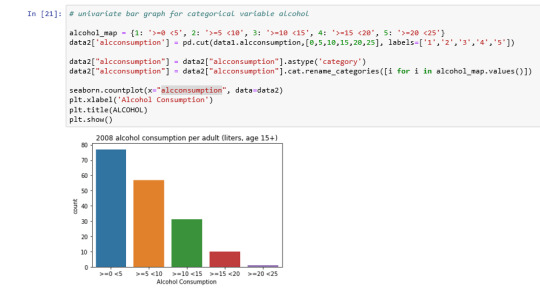
# importing necessary libraries

%matplotlib inline import pandas as pd import numpy as np from collections import OrderedDict from tabulate import tabulate, tabulate_formats import seaborn import matplotlib.pyplot as plt

# bug fix for display formats to avoid run time errors pd.set_option('display.float_format', lambda x:'%f'%x) # Load from CSV

data1 = pd.read_csv('D:/CourseEra/gapminder.csv', skip_blank_lines=True,                   usecols=['country',                             'alcconsumption', 'lifeexpectancy']) data1=data1.replace(r'^\s*$', np.nan, regex=True) data1 = data1.dropna(axis=0, how='any') # Variables Descriptions ALCOHOL = "2008 alcohol consumption per adult (liters, age 15+)" LIFE = "2011 life expectancy at birth (years)" for dt in ( 'alcconsumption', 'lifeexpectancy') :     data1[dt] = pd.to_numeric(data1[dt], 'errors=coerce') data2 = data1.copy()

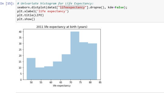
#Univariate histogram for alcohol consumption: seaborn.distplot(data1["alcconsumption"].dropna(), kde=False); plt.xlabel('alcohol consumption (liters)') plt.title(ALCOHOL) plt.show()

The univariate graph of alcohol consumption :

The Univariate Graph of Life Expectancy:

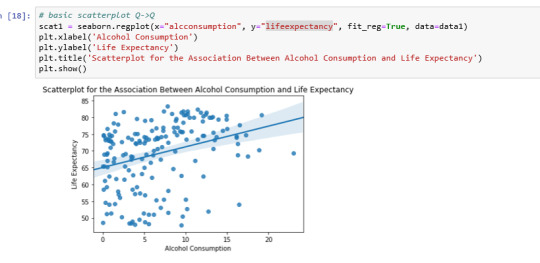
Scatterplot for the association between Alcohol Consumption and Life Expectancy:

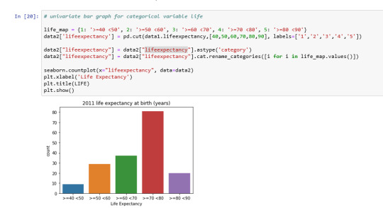
Univariate bar graph for categorical variable life expectancy:

Univariate bar graph for categorical variable alcohol consumption:

Bivariate bar graph

Analyzing only the scatter graph seems do not be a correlation between the variables, but considering the bivariate bar graph, we can say that moderate alcohol consumption can contribute to life expectancy increases. Of course, this is not a scientific work and have value only for this context.

[jebadeiah]

(Day 7) Cleanin' up the CRUD

(Day 7) Cleanin’ up the CRUD

Hi Michael. This is going to be another shorter one, so let’s knock it out.

#!usr/bin/env python3 from collections import OrderedDict import datetime import sys from peewee import * db = SqliteDatabase("diary.db") class Entry(Model): content = TextField() timestamp = DateTimeField(default=datetime.datetime.now) class Meta: database = db def initialize(): """Create thedatabase and the table if…

[drsuthar]

Week 1:Machine Learning - Decision Trees

This is the first task of the Machine Learning Course.

Here are my variables:

Income , which is an Explanatory Variable Alcohol, also an Explanatory Variable Life, which is a Response Variable

Decision Tree

This is how the decision tree looks like :

Interpretation:

The result tree starts with the split on income variable, my second explanatory variable.

This binary variable has values of zero (0) representing income level less than or equals the mean  and value one (1) representing income greater than the mean.

In the first split we can see that 26 countries have the life expectancy and income levels greater than the mean and the other 76 countries have the life expectancy less than the mean.  

The second split , splits in the other the nodes according to consumption alcohol levels and so on.

we can see that the majority of countries with the life expectancy greater than the mean  has the alcohol consumption between 2.5 and 3.5 liters per year

Code:

import pandas as pd import numpy as np from collections import OrderedDict import matplotlib.pyplot as plt from sklearn.cross_validation import train_test_split from sklearn.tree import DecisionTreeClassifier from sklearn.metrics import classification_report import sklearn.metrics

from sklearn import tree from io import StringIO from IPython.display import Image import pydotplus import itertools

# Variables Descriptions INCOME = “2010 Gross Domestic Product per capita in constant 2000 US$” ALCOHOL = “2008 alcohol consumption (litres, age 15+)” LIFE = “2011 life expectancy at birth (years)”

# bug fix for display formats to avoid run time errors pd.set_option(‘display.float_format’, lambda x:’%f’%x)

# Load from CSV data = pd.read_csv('gapminder.csv’, skip_blank_lines=True,                    usecols=['country’,'incomeperperson’,                             'alcconsumption’,'lifeexpectancy’])

data.columns = ['country’,'income’,'alcohol’,'life’]

# converting to numeric values and parsing (numeric invalids=NaN) # convert variables to numeric format using convert_objects function data['alcohol’]=pd.to_numeric(data['alcohol’],errors='coerce’) data['income’]=pd.to_numeric(data['income’],errors='coerce’) data['life’]=pd.to_numeric(data['life’],errors='coerce’)

# Remove rows with nan values data = data.dropna(axis=0, how='any’)

# Copy dataframe for preserve original data1 = data.copy()

# Mean, Min and Max of life expectancy# Mean, meal = data1.life.mean() minl = data1.life.min() maxl = data1.life.max()

# Create categorical response variable life (Two levels based on mean) data1['life’] = pd.cut(data.life,[np.floor(minl),meal,np.ceil(maxl)], labels=[’<=69’,’>69’]) data1['life’] = data1['life’].astype('category’)

# Mean, Min and Max of alcohol meaa = data1.alcohol.mean() mina = data1.alcohol.min() maxa = data1.alcohol.max()

# Categoriacal explanatory variable (Two levels based on mean) data1['alcohol’] = pd.cut(data.alcohol,[np.floor(mina),meaa,np.ceil(maxa)],                         labels=[0,1])

cat1 = pd.cut(data.alcohol,5).cat.categories data1[“alcohol”] = pd.cut(data.alcohol,5,labels=['0’,'1’,'2’,'3’,'4’]) data1[“alcohol”] = data1[“alcohol”].astype('category’)

# Mean, Min and Max of income meai = data1.income.mean() mini = data1.income.min() maxi = data1.income.max()

# Categoriacal explanatory variable (Two levels based on mean) data1['income’] = pd.cut(data.income,[np.floor(mini),meai,np.ceil(maxi)],                         labels=[0,1]) data1[“income”] = data1[“income”].astype('category’)

# convert variables to numeric format using convert_objects function data1['alcohol’]=pd.to_numeric(data1['alcohol’],errors='coerce’) data1['income’]=pd.to_numeric(data1['income’],errors='coerce’)

data1 = data1.dropna(axis=0, how='any’)

predictors = data1[['alcohol’, 'income’]] targets = data1.life pred_train, pred_test, tar_train, tar_test  =   train_test_split(predictors, targets, test_size=.4)

#Build model on training data clf = DecisionTreeClassifier() clf = clf.fit(pred_train,tar_train)

predictions=clf.predict(pred_test)

accuracy = sklearn.metrics.accuracy_score(tar_test, predictions) print ('Accuracy Score: ’, accuracy,’\n’)

#Displaying the decision tree from sklearn import tree #from StringIO import StringIO from io import StringIO #from StringIO import StringIO from IPython.display import Image out = StringIO() tree.export_graphviz(clf, out_file=out) import pydotplus graph=pydotplus.graph_from_dot_data(out.getvalue()) Image(graph.create_png())

[webbazaar0101]

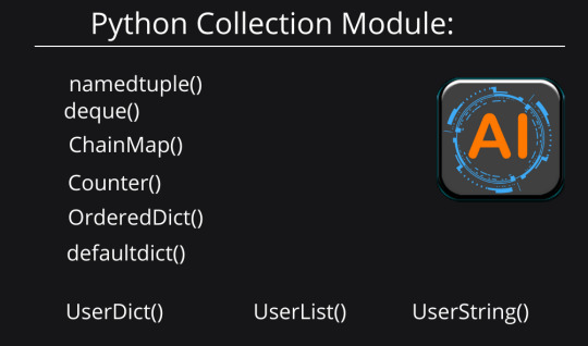
Python Collection Module

Python Collection Module: The collections module provides specialized, high, performance alternatives for the built-in data types as well as a utility function to create named tuples. Python collections improve the functionalities of the built-in....

The collections module provides specialized, high, performance alternatives forthe built-in data types as well as a utility function to create named tuples. Python collections improve the functionalities of the built-in collection containers like list, dictionary, tuple etc. The following table lists the data types and operations of the collections module and their…

[shinjiniandherresearchproje-blog]

Week 4 : logistic regression

I am trying to a logistic regression where ,

Internet usage is my response variable

Electricity Usage is my explanatory variable

and, Urbanization level is also another Explanatory variable

The code is here as follows:

import pandas as pd import numpy as np from collections import OrderedDict import seaborn as sn import matplotlib.pyplot as plt import scipy.stats import statsmodels.formula.api as smf import statsmodels.stats.multicomp as multi import statsmodels.api as sm#call in data set

# Load from CSV data = pd.read_csv('gapminder.csv', skip_blank_lines=True,                     usecols=['country','incomeperperson',                              'urbanrate','relectricperperson', 'internetuserate'])

# Rename columns for clarity                                    

data.columns = ['country','income','internet','electric','urban_rate'] # convert variables to numeric format using convert_objects function data['urban_rate']=pd.to_numeric(data['urban_rate'],errors='coerce') data['income']=pd.to_numeric(data['income'],errors='coerce') data['internet']=pd.to_numeric(data['internet'],errors='coerce')

# Remove rows with nan values

data['electric']=pd.to_numeric(data['electric'],errors='coerce')

# Copy data frame for preserve original

data = data.dropna(axis=0, how='any')

data1 = data.copy()

# Mean, Min and Max of INTERNET USAGE

mean_i= data1.internet.mean() min_i = data1.internet.min() max_i= data1.internet.max()

# Categorical response variable life (Two levels based on mean)

data1['internet'] = pd.cut(data1.internet,[np.floor(min_i),mean_i,np.ceil(max_i)], labels=[0,1]) data1['internet'] = data1['internet'].astype('category')

# Mean, Min and Max of electricity usage

mean_e = data1.electric.mean() min_e = data1.electric.min() max_e = data1.electric.max()

# Categorical explanatory variable electricity usage (Two levels based on mean)

data1['electric'] = pd.cut(data1.electric,[np.floor(min_e),mean_e,np.ceil(max_e)], labels=[0,1]) data1['electric'] = data1['electric'].astype('category')data1 = data1.dropna(axis=0, how='any')# convert variables to numeric

data1['internet']=pd.to_numeric(data1['internet'],errors='coerce')

data1['electric']=pd.to_numeric(data1['electric'],errors='coerce')lreg1 = smf.logit(formula = 'internet ~ electric',data=data1).fit() print (lreg1.summary())print("Odds Ratios") print (np.exp(lreg1.params))params = lreg1.params conf = lreg1.conf_int() conf['OR'] = params conf.columns = ['Lower CI', 'Upper CI', 'OR']print (np.exp(conf))

# Mean, Min and Max of urban rate# Mean,  

mean_u = data1.urban_rate.mean() min_u = data1.urban_rate.min() max_u = data1.urban_rate.max()lreg2 = smf.logit(formula = 'internet ~ electric + urban_rate',data=data1).fit() print (lreg2.summary()) params = lreg2.params conf = lreg2.conf_int() conf['OR'] = params conf.columns = ['Lower CI', 'Upper CI', 'OR']print (np.exp(conf))

   INFERENCE

Electricity usage is a statistically significant parameter in the estimation of Internet usage .It is 151735087877 times more likely that a person with  Internet usage than a person who doesn’t use Internet that much.

After adding urban_rate we see the likeliness increases- Hence this is a proper confounding variable

[ultragodwinnartey]

Data Visualization - Week 3 Assignment

Data management - This management involves making decisions about data, that will help answer the research questions. 

After examining the codebook and frequency distributions, I found out that I have to make some changes.

Rename Variables

Missing Values

Dropping Missing Values

Frequencies Distribution

Grouping Variables

Full Code 

import pandas import numpy from collections import OrderedDict from tabulate import tabulate, tabulate_formats

#import entire dataset to memory data = pandas.read_csv('gapminder_dataset.csv', skip_blank_lines=True,                     usecols=['country','incomeperperson',                              'alcconsumption', 'suicideper100th'])

# Rename columns for clarity                                     data.columns = ['country','income','alcohol','suicide']

# Variables Descriptions ALCOHOL = "2008 alcohol consumption per adult (liters, age 15+)" INCOME = "2010 Gross Domestic Product per capita in constant 2000 US$" SUICIDE = "2005 Suicide, age adjusted, per 100 000"

# Show info about dataset data.info()

#ensure each of these columns are numeric data['income'] = data['income'].convert_objects(convert_numeric=True) data['alcohol'] = data['alcohol'].convert_objects(convert_numeric=True) data['suicide'] = data['suicide'].convert_objects(convert_numeric=True) print (data.info())

# Show missing data sub1 = data[data.income.isnull() | data.suicide.isnull() | data.alcohol.isnull() | data.country.isnull()] print (tabulate(sub1.head(20), headers=['index','Country','Income','Alcohol','Suicide']))

#removing entries with missing data data = data.dropna(axis=0, how='any') print (data.info())

# absolute Frequency distributions freq_suicide_n = data.suicide.value_counts(sort=False) freq_income_n = data.income.value_counts(sort=False) freq_alcohol_n = data.alcohol.value_counts(sort=False)

print (' Frequency Distribution (first 5)') print ('\nsuicide  ('+SUICIDE+'):') print ( tabulate([freq_suicide_n.head(5)], tablefmt="fancy_grid", headers=([i for i in freq_suicide_n.index])) ) print ('\nincome  ('+INCOME+'):') print ( tabulate([freq_income_n.head(5)], tablefmt="fancy_grid", headers=([i for i in freq_income_n.index])) ) print ('\nalcohol  ('+ALCOHOL+'):') print ( tabulate([freq_suicide_n.head(5)], tablefmt="fancy_grid", headers=([i for i in freq_suicide_n.index])) )

# Min and Max continuous variables: min_max = OrderedDict() dict1 = OrderedDict()

dict1['min'] = data.suicide.min() dict1['max'] = data.suicide.max() min_max['suicide'] = dict1

dict2 = OrderedDict() dict2['min'] = data.income.min() dict2['max'] = data.income.max() min_max['income'] = dict2

dict3 = OrderedDict() dict3['min'] = data.alcohol.min() dict3['max'] = data.alcohol.max() min_max['alcohol'] = dict3

df = pandas.DataFrame([min_max['income'],min_max['suicide'],min_max['alcohol']], index = ['Income','suicide','Alcohol']) print (tabulate(df.sort_index(axis=1, ascending=False), headers=['Var','Min','Max']))

data2 = data.copy()

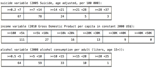
# Maps income_map = {1: '>=100  <5k', 2: '>=5k <10k', 3: '>=10k <20k',               4: '>=20K <30K', 5: '>=30K <40K', 6: '>=40K <50K' } suicide_map = {1: '>=0.2 <7', 2: '>=7 <14', 3: '>=14 <21', 4: '>=21 <28', 5: '>=28 <37'} alcohol_map = {1: '>=0.5 <5', 2: '>=5 <10', 3: '>=10 <15', 4: '>=15 <20', 5: '>=20 <25'}

data2['income'] = pandas.cut(data.income,[100,5000,10000,20000,30000,40000,50000], labels=['1','2','3','4','5','6        ']) print (tabulate(data2.head(10),headers='keys'))

data2['suicide'] = pandas.cut(data.suicide,[0.2,7,14,21,28,37], labels=['1','2','3','4','5']) print (tabulate(data2.head(10),headers='keys'))

data2['alcohol'] = pandas.cut(data.alcohol,[0.5,5,10,15,20,25], labels=['1','2','3','4','5']) print (tabulate(data2.head(10),headers='keys'))

# absolute Frequency distributions freq_suicide_n = data2.suicide.value_counts(sort=False) freq_income_n = data2.income.value_counts(sort=False) freq_alcohol_n = data2.alcohol.value_counts(sort=False)

print ('* Absolute Frequencies *') print ('\nsuicide variable ('+SUICIDE+'):') print( tabulate([freq_suicide_n], tablefmt="fancy_grid", headers=(suicide_map.values()))) print ('\nincome variable ('+INCOME+'):') print( tabulate([freq_income_n], tablefmt="fancy_grid", headers=(income_map.values()))) print ('\nalcohol variable ('+ALCOHOL+'):') print( tabulate([freq_alcohol_n], tablefmt="fancy_grid", headers=(alcohol_map.values())))

Break Down of Code and Results

STEP 1: Make and implement data management decisions for the variables you selected.

# Show info about dataset data.info()

#ensure each of these columns are numeric data['income'] = data['income'].convert_objects(convert_numeric=True) data['alcohol'] = data['alcohol'].convert_objects(convert_numeric=True) data['suicide'] = data['suicide'].convert_objects(convert_numeric=True) print (data.info())

# Data management decision to show missing Variables

# Show missing data

sub1 = data[data.income.isnull() | data.suicide.isnull() | data.alcohol.isnull() | data.country.isnull()] print (tabulate(sub1.head(20), headers=['index','Country','Income','Alcohol','Suicide'])

#removing entries with missing data

data = data.dropna(axis=0, how='any')

print (data.info())

STEP 2: Run frequency distributions for your chosen variables and select columns, and possibly rows.

# Frequency distributions (first 5)

freq_suicide_n = data.suicide.value_counts(sort=False) freq_income_n = data.income.value_counts(sort=False) freq_alcohol_n = data.alcohol.value_counts(sort=False)

print (' Frequencie Distribution (first 5)') print ('\nsuicide  ('+SUICIDE+'):') print ( tabulate([freq_suicide_n.head(5)], tablefmt="fancy_grid", headers=([i for i in freq_suicide_n.index])) ) print ('\nincome  ('+INCOME+'):') print ( tabulate([freq_income_n.head(5)], tablefmt="fancy_grid", headers=([i for i in freq_income_n.index])) ) print ('\nalcohol  ('+ALCOHOL+'):') print ( tabulate([freq_suicide_n.head(5)], tablefmt="fancy_grid", headers=([i for i in freq_suicide_n.index])) )

# Data management decision to group Variables

# grouping results (first calculate the min and max values of each variable)

min_max = OrderedDict() dict1 = OrderedDict()

dict1['min'] = data.suicide.min() dict1['max'] = data.suicide.max() min_max['suicide'] = dict1

dict2 = OrderedDict() dict2['min'] = data.income.min() dict2['max'] = data.income.max() min_max['income'] = dict2

dict3 = OrderedDict() dict3['min'] = data.alcohol.min() dict3['max'] = data.alcohol.max() min_max['alcohol'] = dict3

df = pandas.DataFrame([min_max['income'],min_max['suicide'],min_max['alcohol']], index = ['Income','suicide','Alcohol']) print (tabulate(df.sort_index(axis=1, ascending=False), headers=['Var','Min','Max']))

#Data Dictionary (creating ranges based on min and max values)

income_map = {1: '>=100  <5k', 2: '>=5k <10k', 3: '>=10k <20k',              4: '>=20K <30K', 5: '>=30K <40K', 6: '>=40K <50K' } suicide_map = {1: '>=0.2 <7', 2: '>=7 <14', 3: '>=14 <21', 4: '>=21 <28', 5: '>=28 <37'} alcohol_map = {1: '>=0.5 <5', 2: '>=5 <10', 3: '>=10 <15', 4: '>=15 <20', 5: '>=20 <25'}

#Print first 10 lines of dataset based on new categories

data2['income'] = pandas.cut(data.income,[100,5000,10000,20000,30000,40000,50000], labels=['1','2','3','4','5','6        ']) print (tabulate(data2.head(10),headers='keys'))

data2['suicide'] = pandas.cut(data.suicide,[0.2,7,14,21,28,37], labels=['1','2','3','4','5']) print (tabulate(data2.head(10),headers='keys'))

data2['alcohol'] = pandas.cut(data.alcohol,[0.5,5,10,15,20,25], labels=['1','2','3','4','5']) print (tabulate(data2.head(10),headers='keys'))

#frequency distributions for the new categorical variables

[webscreenscraping]

How Web Scraping Is Used To Extract Yahoo Finance Data: Stock Prices, Bids, Price Change And More?

The stock market is a massive database for technological companies, with millions of records that are updated every second! Because there are so many companies that provide financial data, it's usually done through Real-time web scraping API, and APIs always have premium versions. Yahoo Finance is a dependable source of stock market information. It is a premium version because Yahoo also has an API. Instead, you can get free access to any company's stock information on the website.

Although it is extremely popular among stock traders, it has persisted in a market when many large competitors, including Google Finance, have failed. For those interested in following the stock market, Yahoo provides the most recent news on the stock market and firms.

Steps to Scrape Yahoo Finance

Create the URL of the search result page from Yahoo Finance.

Download the HTML of the search result page using Python requests.

Scroll the page using LXML-LXML and let you navigate the HTML tree structure by using Xpaths. We have defined the Xpaths for the details we need for the code.

Save the downloaded information to a JSON file.

We will extract the following data fields:

Previous close

Open

Bid

Ask

Day’s Range

52 Week Range

Volume

Average volume

Market cap

Beta

PE Ratio

1yr Target EST

You will need to install Python 3 packages for downloading and parsing the HTML file.

The Script

from lxml import html import requests import json import argparse from collections import OrderedDict def get_headers(): return {"accept": "text/html,application/xhtml+xml,application/xml;q=0.9,image/webp,image/apng,*/*;q=0.8,application/signed-exchange;v=b3;q=0.9", "accept-encoding": "gzip, deflate, br", "accept-language": "en-GB,en;q=0.9,en-US;q=0.8,ml;q=0.7", "cache-control": "max-age=0", "dnt": "1", "sec-fetch-dest": "document", "sec-fetch-mode": "navigate", "sec-fetch-site": "none", "sec-fetch-user": "?1", "upgrade-insecure-requests": "1", "user-agent": "Mozilla/5.0 (Windows NT 10.0; Win64; x64) AppleWebKit/537.36 (KHTML, like Gecko) Chrome/81.0.4044.122 Safari/537.36"} def parse(ticker): url = "http://finance.yahoo.com/quote/%s?p=%s" % (ticker, ticker) response = requests.get( url, verify=False, headers=get_headers(), timeout=30) print("Parsing %s" % (url)) parser = html.fromstring(response.text) summary_table = parser.xpath( '//div[contains(@data-test,"summary-table")]//tr') summary_data = OrderedDict() other_details_json_link = "https://query2.finance.yahoo.com/v10/finance/quoteSummary/{0}?formatted=true&lang=en-US®ion=US&modules=summaryProfile%2CfinancialData%2CrecommendationTrend%2CupgradeDowngradeHistory%2Cearnings%2CdefaultKeyStatistics%2CcalendarEvents&corsDomain=finance.yahoo.com".format( ticker) summary_json_response = requests.get(other_details_json_link) try: json_loaded_summary = json.loads(summary_json_response.text) summary = json_loaded_summary["quoteSummary"]["result"][0] y_Target_Est = summary["financialData"]["targetMeanPrice"]['raw'] earnings_list = summary["calendarEvents"]['earnings'] eps = summary["defaultKeyStatistics"]["trailingEps"]['raw'] datelist = [] for i in earnings_list['earningsDate']: datelist.append(i['fmt']) earnings_date = ' to '.join(datelist) for table_data in summary_table: raw_table_key = table_data.xpath( './/td[1]//text()') raw_table_value = table_data.xpath( './/td[2]//text()') table_key = ''.join(raw_table_key).strip() table_value = ''.join(raw_table_value).strip() summary_data.update({table_key: table_value}) summary_data.update({'1y Target Est': y_Target_Est, 'EPS (TTM)': eps, 'Earnings Date': earnings_date, 'ticker': ticker, 'url': url}) return summary_data except ValueError: print("Failed to parse json response") return {"error": "Failed to parse json response"} except: return {"error": "Unhandled Error"} if __name__ == "__main__": argparser = argparse.ArgumentParser() argparser.add_argument('ticker', help='') args = argparser.parse_args() ticker = args.ticker print("Fetching data for %s" % (ticker)) scraped_data = parse(ticker) print("Writing data to output file") with open('%s-summary.json' % (ticker), 'w') as fp: json.dump(scraped_data, fp, indent=4)

Executing the Scraper

Assuming the script is named yahoofinance.py. If you type in the code name in the command prompt or terminal with a -h.

python3 yahoofinance.py -h usage: yahoo_finance.py [-h] ticker positional arguments: ticker optional arguments: -h, --help show this help message and exit

The ticker symbol, often known as a stock symbol, is used to identify a corporation.

To find Apple Inc stock data, we would make the following argument:

python3 yahoofinance.py AAPL

This will produce a JSON file named AAPL-summary.json in the same folder as the script.

This is what the output file would look like:

{ "Previous Close": "293.16", "Open": "295.06", "Bid": "298.51 x 800", "Ask": "298.88 x 900", "Day's Range": "294.48 - 301.00", "52 Week Range": "170.27 - 327.85", "Volume": "36,263,602", "Avg. Volume": "50,925,925", "Market Cap": "1.29T", "Beta (5Y Monthly)": "1.17", "PE Ratio (TTM)": "23.38", "EPS (TTM)": 12.728, "Earnings Date": "2020-07-28 to 2020-08-03", "Forward Dividend & Yield": "3.28 (1.13%)", "Ex-Dividend Date": "May 08, 2020", "1y Target Est": 308.91, "ticker": "AAPL", "url": "http://finance.yahoo.com/quote/AAPL?p=AAPL" }

This code will work for fetching the stock market data of various companies. If you wish to scrape hundreds of pages frequently, there are various things you must be aware of.

Why Perform Yahoo Finance Data Scraping?

If you're working with stock market data and need a clean, free, and trustworthy resource, Yahoo Finance might be the best choice. Different company profile pages have the same format, thus if you construct a script to scrape data from a Microsoft financial page, you could use the same script to scrape data from an Apple financial page.

If anyone is unable to choose how to scrape Yahoo finance data then it is better to hire an experienced web scraping company like Web Screen Scraping.

For any queries, contact Web Screen Scraping today or Request for a free Quote!!