#adjoint matrix

[peeterjoot]

Simplifying the previous adjoint matrix results.

[Click here for a PDF version of this (and the previous) post] We previously found determinant expressions for the matrix elements of the adjoint for 2D and 3D matrices \( M \). However, we can extract additional structure from each of those results. 2D case. Given a matrix expressed in block matrix form in terms of it’s columns \begin{equation}\label{eqn:adjoint:500} M = \begin{bmatrix} \Bm_1 &…

[golzarrahman66-blog]

https://mathgr.com/grpost.php?grtid=3

ম্যাট্রিক্স ও নির্ণায়ক এর মধ্যে পার্থক্য কী?, ব্যাতিক্রমী ও অব্যাতিক্রমী ম্যাট্রিক্স কী?, বর্গ ম্যাট্রিক্সের বিপরীত ম্যাট্রিক্স কী?, বর্গ ম্যাট্রিক্সের অ্যাডজয়েন্ট কী?, বিপরীত ম্যাট্রিক্সের বৈশিষ্ট কী?, অর্থোগোনাল ম্যাট্রিক্স কী?, একঘাত সমীকরণ জোট ও এর সমাধান কী?, ক্রেমারের নিয়মে একঘাত সমীকরণ জোটের সমাধান কী?, তিন চলকবিশিষ্ট একঘাত সমীকরণ জোটের সমাধান বিপরীত ম্যাট্রিক্সের সাহায্যে একঘাত সমীকরণ জোটের সমাধান কী?, বর্গ ম্যাট্রিক্সের ট্রেস কী?, Defference between Matrix and Determinant, Singular and Non-Singular Matrix, Inverse Matrix of a Square Matrix, Adjoint of a Square Matrix, Properties of Inverse Matrix, Orthogonal Matrix, System of linear equations and it's solution, Solution of system of linear equations using cramer's rule, Solution of system of linear equations using inverse myatrix, Trace of Square Matrix

[codingprolab]

CS 3430: SciComp with Py Assignment 6 Determinants, Inverses, and Cramer’s Rule

1 Learning Objectives 1. Determinants 2. Matrix Inverse 3. Cramer’s Rule 4. Solving Square Linear Systems 5. Numpy 2 Introduction We will stay with linear algebra in this assignment to learn how to compute determinants, adjoint matrices, and to use Cramer’s rule to solve square linear systems. In 2D and 3D, determinants are areas and volumes. In m-dimensional spaces, determinants are critical in…

[physicsforever]

Derivation of Cayley Hamilton Theorem I Using Adjoint Matrix I PGTRB I P...

[sethiswiftlearn]

Class 12 Math | Matrices and Determinants part 2 | JEE Mains, CUET Prep

Matrices and Determinants are fundamental topics in Class 12 Mathematics, playing a crucial role in algebra and real-world applications. Mastering these concepts is essential for students preparing for competitive exams like JEE Mains, CUET, and other entrance tests. In this session, we continue exploring Matrices and Determinants (Part 2) with a deep dive into advanced concepts, problem-solving techniques, and shortcuts to enhance your mathematical skills.

What You’ll Learn in This Session?

In this second part of Matrices and Determinants, we cover: ✔ Types of Matrices & Their Properties – Understanding singular and non-singular matrices, symmetric and skew-symmetric matrices, and orthogonal matrices. ✔ Elementary Operations & Inverse of a Matrix – Step-by-step method to compute the inverse of a matrix using elementary transformations and properties of matrix operations. ✔ Adjoint and Cofactor of a Matrix – Learn how to find the adjoint and use it to compute the inverse efficiently. ✔ Determinants & Their Applications – Mastery of determinant properties and how they apply to solving equations. ✔ Solving Linear Equations using Matrices – Application of matrices in solving system of linear equations using Cramer’s Rule and Matrix Inversion Method. ✔ Shortcut Techniques & Tricks – Learn time-saving strategies to tackle complex determinant and matrix problems in exams.

Why is This Session Important?

Matrices and Determinants are not just theoretical concepts; they have wide applications in physics, computer science, economics, and engineering. Understanding their properties and operations simplifies problems in linear algebra, calculus, and probability. This topic is also heavily weighted in JEE Mains, CUET, and CBSE Board Exams, making it vital for scoring well.

Who Should Watch This?

JEE Mains Aspirants – Get an edge with advanced problem-solving strategies.

CUET & Other Competitive Exam Candidates – Build a strong foundation for entrance exams.

Class 12 CBSE & State Board Students – Strengthen concepts and improve exam performance.

Anyone Seeking Concept Clarity – If you want to master Matrices and Determinants, this session is perfect for you!

How Will This Help You?

Conceptual Clarity – Develop a clear understanding of matrices, their types, and operations.

Stronger Problem-Solving Skills – Learn various techniques and tricks to solve complex determinant problems quickly.

Exam-Focused Approach – Solve previous years' JEE Mains, CUET, and CBSE board-level questions.

Step-by-Step Explanations – Get detailed solutions to frequently asked questions in competitive exams.

Watch Now & Strengthen Your Math Skills!

Don't miss this in-depth session on Matrices and Determinants (Part 2). Strengthen your concepts, learn effective shortcuts, and boost your problem-solving skills to ace JEE Mains, CUET, and board exams.

📌 Watch here 👉 https://youtu.be/

🔔 Subscribe for More Updates! Stay tuned for more quick revision sessions, concept explanations, and exam tricks to excel in mathematics.

[generating-functionology]

okay. Analysis went slightly better today than yesterday (borderline pass/fail), but unfortunately there is a lot of work to do. I think I'm going to try and also do some problems from yesterday in algebra I didn't get to, as well as look at problems on a particularly difficult exam me and another classmate struggled with.

Things I need to address in analysis:

Sequential compactness, multivariable calculus, fundamental theorem of calculus.

In algebra:

Jordan forms, generalized eigenspaces, proving the existence of eigenvalues without using the fundamental theorem of algebra (for self-adjoint real symmetric matrices.)

Also rank is always annoying. I also need to review and internalize the explicit conditions for the complex and real spectral theorems and why T self-adjoint -> Upper-triangular matrix with respect to some basis -> diagonal matrix with respect to some orthonormal basis -> has a basis consisting of eigenvectors of T.

I think today would be a good day to review and practice proving major theorems and reinforce learning techniques instead of going crazy on exam problems all day - I'll save the exam problems for the evening.

[erikabsworld]

Unraveling the Complexity of Matrix Algebra Assignments

Matrix algebra can often be likened to a labyrinth of abstract concepts and intricate calculations, leaving many students feeling lost and overwhelmed. In this blog, we'll unravel the complexities of matrix algebra by dissecting a challenging university-level assignment question and providing a step-by-step guide to its solution. So, let's embark on this journey to demystify matrix algebra and equip you with the tools to conquer even the toughest assignments.

The Question:

Consider a square matrix A of order 3x3. Determine whether A is invertible or not. If invertible, find its inverse matrix. If not, explain why.

Conceptual Overview:

Before diving into the solution, let's grasp the fundamental concept at play: invertibility of matrices. In matrix algebra, a square matrix is considered invertible, or non-singular, if it possesses an inverse matrix. This inverse matrix, when multiplied by the original matrix, yields the identity matrix. If a matrix lacks an inverse, it is deemed singular.

Step-by-Step Solution:

Calculate the Determinant: Begin by computing the determinant of matrix A. The determinant serves as a crucial determinant of invertibility. If the determinant is non-zero, the matrix is invertible; otherwise, it's not.

Evaluate Invertibility: Determine whether the calculated determinant is non-zero. If it is, then A is invertible. If the determinant equals zero, A is singular and lacks an inverse.

Finding the Inverse (if applicable): If A is invertible, proceed to find its inverse using suitable methods such as adjoint method or Gauss-Jordan elimination. The inverse matrix A^{-1} satisfies the condition AA^−1=A^−1 A=I, where I is the identity matrix.

How We Can Help:

Navigating through matrix algebra assignments can be challenging, but you don't have to face it alone. At matlabassignmentexperts.com, we offer comprehensive matrix algebra assignment help services tailored to your specific needs. Our team of experienced tutors is dedicated to providing personalized guidance and support, ensuring you grasp the concepts and excel in your studies. From conceptual explanations to step-by-step solutions, we're here to empower you on your academic journey.

Conclusion:

Matrix algebra may seem daunting at first glance, but with a clear understanding of its fundamental principles and problem-solving techniques, you can unravel its complexities. By following the step-by-step guide provided in this blog, you'll be well-equipped to tackle challenging assignments with confidence. Remember, perseverance and seeking help when needed are key to mastering matrix algebra and achieving academic success.

[lawsofemotion]

Finished Chapter 2: Determinants!

Questions, comments, corrections? Message me here or on the other blog!

[peeterjoot]

Computing the adjoint matrix

[Click here for a PDF version of this post] I started reviewing a book draft that mentions the adjoint in passing, but I’ve forgotten what I knew about the adjoint (not counting self-adjoint operators, which is different.) I do recall that adjoint matrices were covered in high school linear algebra (now 30+ years ago!), but never really used after that. It appears that the basic property of the…

[basictutor]

Adjoint of a 2x2 Matrix

Adjoint of a 2×2 Matrix

[renatoferreiradasilva]

Spectral Modeling of Riemann Zeta Zeros Using Schrödinger Operators and Machine Learning

Author: Renato Ferreira da Silva Email: renatoferreiradasilva1980@yahoo.com ORCID: 0009-0003-8908-481X

Abstract: This paper explores a computational approach to approximating the nontrivial zeros of the Riemann zeta function as the spectrum of a self-adjoint operator. Using Schrödinger operators with potentials expanded in a Hermite basis, we train neural networks to infer eigenvalues from parametric potentials and validate their spacing statistics against the Gaussian Unitary Ensemble (GUE) predictions from random matrix theory. The model's robustness is tested with real zeros obtained by Odlyzko, and the methodology is extended to integro-differential operators. The results show numerical compatibility with the Hilbert–Pólya conjecture and open directions for a spectral interpretation of the Riemann Hypothesis.

1. Introduction

The Riemann Hypothesis (RH), one of the most profound problems in mathematics, conjectures that all nontrivial zeros ρ=12+iγj of the Riemann zeta function lie on the critical line ℜ(s)=1/2. An influential perspective known as the Hilbert–Pólya conjecture proposes that these zeros are the eigenvalues of a self-adjoint operator, potentially linking number theory to spectral theory and quantum mechanics. Inspired by this idea, we develop a framework that constructs operators whose spectra approximate these zeros, leveraging numerical methods and machine learning to bridge analytic number theory and physics.

2. Spectral Formulation

We model the operator as a one-dimensional Schrödinger operator:L=−d2dx2+V(x),x∈[−L,L],

with Dirichlet boundary conditions. The potential V(x) is smooth and rapidly decaying, approximated using a Hermite basis:V(x)=∑n=0KcnHn(x)e−x2/2,

where Hn(x) are Hermite polynomials and cn are trainable coefficients. This choice imposes regularity and controls the model's complexity.

3. Numerical Framework and Dataset Generation

The operator is discretized via central differences on a grid with N points. The Laplacian becomes tridiagonal, and the potential is diagonalized using SciPy's sparse eigenvalue solver. Each potential V(x) is generated by sampling the coefficients cn∼N(0,σ2/(1+n)2). The first M eigenvalues are retained for analysis. A logarithmic transformation is applied to improve stability and convergence in training.

4. Neural Network Modeling

A multilayer perceptron (MLP) is trained to map cn→λj with:

Input: 10 coefficients c0,...,c9

Hidden layers: Two with 64 neurons (activation: tanh)

Output: First 50 eigenvalues

Normalization and dropout are applied, and training uses the Adam optimizer. The network achieves MSE below 10−2 on validation data.

5. Statistical Validation via GUE

The eigenvalue spacings are compared with the GUE prediction:PGUE(s)=32π2s2e−4s2/π.

Spacing histograms match the GUE distribution. Kolmogorov–Smirnov tests yield p-values above 0.1. Rigidity statistics further confirm GUE-like behavior.

6. Real Zeros and Inverse Modeling

We replace model spectra with the first 50 real zeros from Odlyzko’s tables and invert the map γj→cn via optimization. The resulting potentials exhibit chaotic, decaying profiles. GUE behavior persists even in these real-data inversions.

7. Extension to Nonlocal Operators

We introduce a nonlocal operator:Lψ(x)=−ψ′′(x)+∫−LLK(x,y)ψ(y) dy,

where K(x,y) is expanded in Hermite functions. These operators connect to Alain Connes’ noncommutative geometry. Preliminary results show GUE statistics emerge from well-chosen kernels.

8. Conclusion and Outlook

This framework blends Schrödinger operators, Hermite expansions, and deep learning to model the Riemann zeros. Future directions include:

Spectral inversion via attention networks or VAEs

Generalization to Dirichlet L-functions

Noncommutative geometry and spectral triples

Stability analysis under potential perturbations

Inverse spectral uniqueness studies

Acknowledgments

The author acknowledges Odlyzko’s dataset and thanks collaborators in spectral geometry and numerical analysis. Supported in part by [Funding Agency, Grant Number].

References

A. M. Odlyzko, The $10^{20}$-th Zero of the Riemann Zeta Function, 1992.

M. V. Berry, J. P. Keating, The Riemann Zeros and Eigenvalue Asymptotics, SIAM Review, 1999.

A. Connes, Noncommutative Geometry, Academic Press, 1994.

T. Tao, Structure and Randomness in the Zeta Function, preprint, 2023.

M. L. Mehta, F. J. Dyson, Statistical Theory of the Energy Levels of Complex Systems, 1963.

M. Raissi et al., Physics-informed neural networks, J. Comput. Phys., 2019.

[mysteriousquantumphysics]

Observable vs. Beable

What is an observable?

Quantum mechanics is primarily described by linear algebra. If you want to know which results you can measure in an experiment you simply calculate the eigenvalues of your observable - a self-adjoint/hermitian operator (effectively a matrix). After the measurement you will find the system in the corresponding eigenstate of the eigenvalue you measured. The wavefunction (that gives us the probabilties of each result) existing before the measurement then has collapsed into this eigenstate. That’s basically it.

Let’s have look on a simple and neat (yet constructed) example: We want to measure the spin in z-direction of a given spin 1/2 system. The corresponding observable consists of the third Pauli matrix and a factor hbar/2 (which is needed because of the dimensions and the fact that the spin is 1/2).

Regarding an arbitrary state that is a linear combination of the basis vectors of this Hilbert space we can get the probability for measuring e.g. s=+hbar/2 by applying the Born rule:

After this measurement any further measurements of the z-component of spin will give us 100% probability to get this spin +1/2 state again - because the given state (linear combination) collapsed. This is more or less the famous collapse of the wavefunction.

But is this all there is?

Those who are not familiar with calculations of the kind as done above might already handle a lot of information at the moment. But now I get to the main point I want to make today: Even someone who just learned the very basics about observables might have a strange feeling about the central term measurement. It invokes the assumption that the act of measurement itself is somehow supposed to be something “fundamental” of nature. But this cannot be the case - the physical world exists without measurement apparatuses and without people who measure. Rather apparatuses and people are part of physical reality as well, what tells us that they should be described by the theory - they should not be a tool of the theory attempting to describe reality. Thus it might be a lot more enlightening to talk about be-ables, rather than only observables; a term introduced by John Bell pointing out the importance of ontology in physical theories. 

When learning the basics of quantum mechanics at university questions of this kind are often discredited as “metaphysical” and thus not worth it to be discussed any further. But do we want to adopt the crude “instrumentalism”, which means that physics shall only be about predictions of results of measurements? Isn’t physics about understanding the nature of reality? Rather thinking about the beables than just the observables?

Though standard quantum mechanics is a theory that is great at predicting the outcomes of measurements, there are theories of quantum mechanics that reproduce the same predictions and do a lot better at those more fundamental epistemological and ontological questions. I’d like to mention at this point e.g. objective collapse theories and Bohmian mechanics as attempts of more complete quantum theories.

---

Further reading recommendations (especially for those who already knew those simple calculations I did above):

Tim Maudlin -  Local Beables and the Foundations of Physics

John Bell - The Theory of Local Beables

[d-janney]

Assignment 5 Part 1

Assignment 5 has two parts. This first part is my interpretation of the assignment, the second part is a more true version of the assignment’s expectations.

Find the value of inverse of a matrix, determinant of a matrix by using the following values:

A=matrix(1:100, nrow=10) B=matrix(1:1000, nrow=10)

Assign letters to their respective matrix values:

>A <- matrix(1:100, nrow=10)   >B <- matrix(1:1000, nrow=10)

First thoughts: looks like A will be 10 columns and 10 rows with values 1-100; and B will be 100 columns and 10 rows with values 1-1000. In my reading of matrices and their inversion I noted that a matrix must be a square to have an inverse, so I will not be finding the determinant or inverse of matrix B. Here is what matrix A looks like:

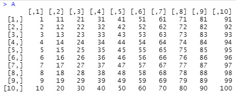
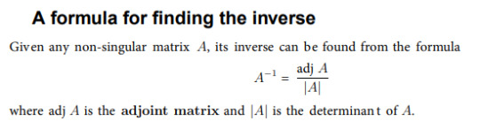
Looking at the “Inverse of a matrix” leaflet, I understand that to find the inverse the adjoint matrix and the determinant are needed.

The adjoint matrix is found by transposing the matrix and creating a matrix of minors and then cofactors. Luckily, R makes this easy to do. To transpose the matrix A, I can include byrow=T to assign the order of values by row instead of column:

Atran <- matrix(1:100, nrow=10, byrow=T)

 Or simply use t() to transpose the matrix:

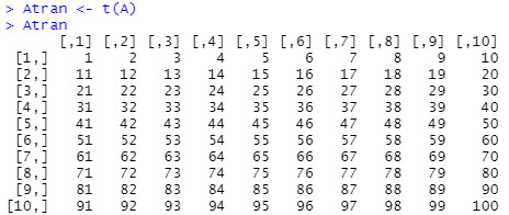
I installed the matlib package in RStudio to help with the matrix functions, especially to find the determinant of matrix A.

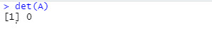
Turns out, matrix A (as it is 1:100) has a determinant of 0, which means its inverse cannot be calculated. So, instead of having an ordered matrix of 1:100, I want to randomize the values to execute the inverse of a matrix and the components related to it. I did this by using sample() and assigned the new matrix values to A2:

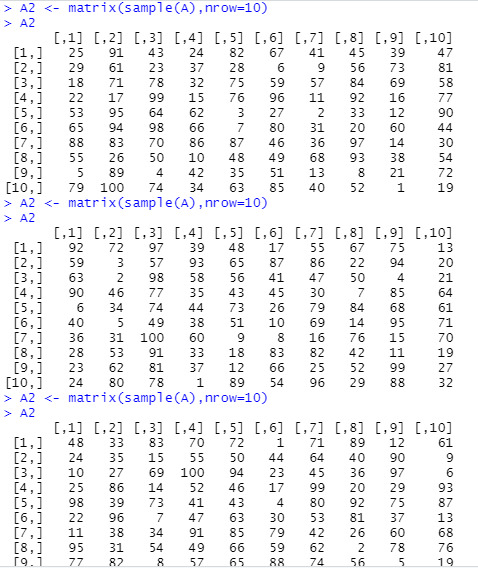
In the graphic above, I ran and printed matrix A2 three separate times to show that each time a different sample of values was made. I encountered this phenomena while experimenting with codes and wanted to show its effects on the data.

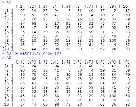
To secure a random sample, I assigned a matrix A3 to a set of A2 data values:

With the A3 matrix, I can find the determinate and inverse using det() and solve():

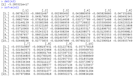
In the determinant value is an “e” and I didn’t know what that meant right away. An internet search has led me to understand -5.285521e+17 as -528,552,100,000,000,000. I think e more likely represents exponent over Euler’s number. 

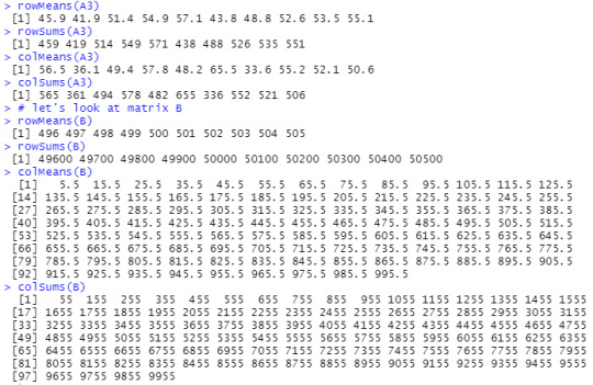
Other mathematical functions that can be applied to a matrix are rowMeans(), rowSums(), colMeans(), and colSums.

[bitrust]

Inverse matrix symbolic calculator

P -1, each component of which can be inexpensively computed (compared to the cost of obtaining the factors).Ī list of 3 Matrices, P, L, U, the PLU decomposition of a Matrix (these are the values returned from LUDecomposition when the output= option is given to that routine). The first member is taken as the pivot Vector and the second member as the superimposed unit-lower and upper triangular LU factors (these are the default values returned from LUDecomposition when the method=NAG option is given to that routine). That is, the list items may be:Ī list of a Vector and Matrix, ipiv, LU, for an LU decomposition. These factors are in the form of returned values from LUDecomposition. If the first argument in the calling sequence is a list, then the elements of the list are taken as the Matrix factors of the Matrix A, due to some prefactorization. The subs method indicates that the input is already triangular, so only the appropriate forward or back substitution is done. The LU and Cholesky methods use the corresponding LUDecomposition method on the input Matrix (if not already prefactored) and then use forward and back substitution with a copy of the identity Matrix as a right-hand side. The polynom method uses an implementation of fraction-free Gaussian elimination. The univar method uses an evaluation method to reduce the Matrix to a Matrix of integers, then uses `Adjoint/integer`, and then uses genpoly to convert back to univariate polynomials. The integer method calls `Adjoint/integer` and divides it by the determinant. The complex and rational methods augment the input Matrix with a copy of the identity Matrix and then convert the system to reduced row echelon form. If m is included in the calling sequence, then the specified method is used to compute the inverse (except for 1 ⁢ x ⁢ 1, 2 ⁢ x ⁢ 2 and 3 ⁢ x ⁢ 3 Matrices where the calculation of the inverse is hard-coded for efficiency). If A is a non-square m ⁢ x ⁢ n Matrix, or if the option method = pseudo is specified, then the Moore-Penrose pseudo-inverse X is computed such that the following identities hold: A -1 = I, where I is the n ⁢ x ⁢ n identity Matrix.If A is a nonsingular n ⁢ x ⁢ n Matrix, the inverse A -1 is computed such that A If A is non-square, the Moore-Penrose pseudo-inverse is returned. If A is recognized as a singular Matrix, an error message is returned. The MatrixInverse(A) function, where A is a nonsingular square Matrix, returns the Matrix inverse A -1. (optional) constructor options for the result object (optional) equation of the form output=obj where obj is 'inverse' or 'proviso' or a list containing one or more of these names selects the result objects to compute (optional) equation of the form conjugate=true or false specifies whether to use the Hermitian transpose in the case of prefactored input from a Cholesky decomposition (optional) equation of the form methodoptions=list where the list contains options for specific methods (optional) equation of the form method = name where name is one of 'LU', 'Cholesky', 'subs', 'integer', 'univar', 'polynom', 'complex', 'rational', 'pseudo', or 'none' method used to factorize the inverse of A MatrixInverse( A, m, mopts, c, out, options ) Compute the inverse of a square Matrix or the Moore-Penrose pseudo-inverse of a Matrix

[healthfitnessidea]

TB Business Mathematics | Pages-540 | Code-661 | Edition-10th| Concepts + Theorems/Derivations + Solved Numericals + Practice Exercises | Text Book

TB Business Mathematics | Pages-540 | Code-661 | Edition-10th| Concepts + Theorems/Derivations + Solved Numericals + Practice Exercises | Text Book

Price: (as of – Details) SYLLABUS- BUSINESS MATHEMATICS, Unit-I Matrix: Introduction, Square Matrix, Row Matrix, Column Matrix, Diagonal Matrix, Identity Matrix, Addition, Subtraction & Multiplication of Matrix, Use of Matrix in Business Mathematical Induction. Unit-II Inverse of Matrix, Rank of Matrix, Solution to a system of equation by the adjoint Matrix Methods & Guassian Elimination…