#install MongoDB in AWS ec2 instance

[govindhtech]

What Is Amazon EBS? Features Of Amazon EBS And Pricing

Amazon Elastic Block Store: High-performance, user-friendly block storage at any size

What is Amazon EBS?

Amazon Elastic Block Store provides high-performance, scalable block storage with Amazon EC2 instances. AWS Elastic Block Store can create and manage several block storage resources:

Amazon EBS volumes: Amazon EC2 instances can use Amazon EBS volumes. A volume associated to an instance can be used to install software and store files like a local hard disk.

Amazon EBS snapshots: Amazon EBS snapshots are long-lasting backups of Amazon EBS volumes. You can snapshot Amazon EBS volumes to backup data. Afterwards, you can always restore new volumes from those snapshots.

Advantages of the Amazon Elastic Block Store

Quickly scale

For your most demanding, high-performance workloads, including mission-critical programs like Microsoft, SAP, and Oracle, scale quickly.

Outstanding performance

With high availability features like replication within Availability Zones (AZs) and io2 Block Express volumes’ 99.999% durability, you can guard against failures.

Optimize cost and storage

Decide which storage option best suits your workload. From economical dollar-per-GB to high performance with the best IOPS and throughput, volumes vary widely.

Safeguard

You may encrypt your block storage resources without having to create, manage, and safeguard your own key management system. Set locks on data backups and limit public access to prevent unwanted access to your data.

Easy data security

Amazon EBS Snapshots, a point-in-time copy that can be used to allow disaster recovery, move data across regions and accounts, and enhance backup compliance, can be used to protect block data storage both on-site and in the cloud. With its integration with Amazon Data Lifecycle Manager, AWS further streamlines snapshot lifecycle management by enabling you to establish policies that automate various processes, such as snapshot creation, deletion, retention, and sharing.

How it functions

A high-performance, scalable, and user-friendly block storage solution, Amazon Elastic Block Store was created for Amazon Elastic Compute Cloud (Amazon EC2).Image credit to AWS

Use cases

Create your cloud-based, I/O-intensive, mission-critical apps

Switch to the cloud for mid-range, on-premises storage area network (SAN) applications. Attach block storage that is both high-performance and high-availability for applications that are essential to the mission.

Utilize relational or NoSQL databases

Install and expand the databases of your choosing, such as Oracle, Microsoft SQL Server, PostgreSQL, MySQL, Cassandra, MongoDB, and SAP HANA.

Appropriately scale your big data analytics engines

Detach and reattach volumes effortlessly, and scale clusters for big data analytics engines like Hadoop and Spark with ease.

Features of Amazon EBS

It offers the following features:

Several volume kinds: Amazon EBS offers a variety of volume types that let you maximize storage efficiency and affordability for a wide range of uses. There are two main sorts of volume types: HDD-backed storage for workloads requiring high throughput and SSD-backed storage for transactional workloads.

Scalability: You can build Amazon EBS volumes with the performance and capacity requirements you want. You may adjust performance or dynamically expand capacity using Elastic Volumes operations as your needs change, all without any downtime.

Recovery and backup: Back up the data on your disks using Amazon EBS snapshots. Those snapshots can subsequently be used to transfer data between AWS accounts, AWS Regions, or Availability Zones or to restore volumes instantaneously.

Data protection: Encrypt your Amazon EBS volumes and snapshots using Amazon EBS encryption. To secure data-at-rest and data-in-transit between an instance and its connected volume and subsequent snapshots, encryption procedures are carried out on the servers that house Amazon EC2 instances.

Data availability and durability: io2 Block Express volumes have an annual failure rate of 0.001% and a durability of 99.999%. With a 0.1% to 0.2% yearly failure rate, other volume types offer endurance of 99.8% to 99.9%. To further guard against data loss due to a single component failure, volume data is automatically replicated across several servers in an Availability Zone.

Data archiving: EBS Snapshots Archive provides an affordable storage tier for storing full, point-in-time copies of EBS Snapshots, which you must maintain for a minimum of ninety days in order to comply with regulations. and regulatory purposes, or for upcoming project releases.

Related services

These services are compatible with Amazon EBS:

In the AWS Cloud, Amazon Elastic Compute Cloud lets you start and control virtual machines, or EC2 instances. Like hard drives, EBS volumes may store data and install software.

You can produce and maintain cryptographic keys with AWS Key Management Service, a managed service. Data saved on your Amazon EBS volumes and in your Amazon EBS snapshots can be encrypted using AWS KMS cryptographic keys.

EBS snapshots and AMIs supported by EBS are automatically created, stored, and deleted with Amazon Data Lifecycle Manager, a managed service. Backups of your Amazon EC2 instances and Amazon EBS volumes can be automated with Amazon Data Lifecycle Manager.

EBS direct APIs: These services let you take EBS snapshots, write data to them directly, read data from them, and determine how two snapshots differ or change from one another.

Recycle Bin is a data recovery solution that lets you recover EBS-backed AMIs and mistakenly erased EBS snapshots.

Accessing Amazon EBS

The following interfaces are used to build and manage your Amazon EBS resources:

Amazon EC2 console

A web interface for managing and creating snapshots and volumes.

AWS Command Line Interface

A command-line utility that enables you to use commands in your command-line shell to control Amazon EBS resources. Linux, Mac, and Windows are all compatible.

AWS Tools for PowerShell

A set of PowerShell modules for scripting Amazon EBS resource activities from the command line.

Amazon CloudFormation

It’s a fully managed AWS service that allows you describe your AWS resources using reusable JSON or YAML templates, and then it will provision and setup those resources for you.

Amazon EC2 Query API

The HTTP verbs GET or POST and a query parameter called Action are used in HTTP or HTTPS requests made through the Amazon EC2 Query API.

Amazon SDKs

APIs tailored to particular languages that let you create apps that interface with AWS services. Numerous well-known programming languages have AWS SDKs available.

Amazon EBS Pricing

You just pay for what you provision using Amazon EBS. See Amazon EBS pricing for further details.

Read more on Govindhtech.com

[tastethelinux]

Install MongoDB on AWS EC2 Instances.

Install MongoDB on AWS EC2 Instances.

We will see how to install MongoDB on AWS ec2 Instances, amazon Linux 2 or we can install MongoDB of any version on the AWS Linux 2 server in this article. The Amazon Linux 2 server is the RPM-based server with the 5 years Long Term Support by AWS. (Amazon Web Services). MongoDB is a No-SQL database which is written in C++, It uses a JSON like structure. MongoDB is a cross-platform and…

[pinerrelief]

1 and 1 bitnami mean ssl

1 AND 1 BITNAMI MEAN SSL HOW TO

1 AND 1 BITNAMI MEAN SSL INSTALL

1 AND 1 BITNAMI MEAN SSL UPDATE

Im also looking forward to branching out and trying the Wordpress, Ghost, and Magento stacks as well. 0 5 1 /home/bitnami/letsencrypt/letsencrypt-auto renew sudo /opt/bitnami/ctlscript.sh restart.

1 AND 1 BITNAMI MEAN SSL INSTALL

Do you have any favorite stacks/apps So far, Ive had great success with the Bitnami MEAN stack in AWS. Install Letsencrypt SSL to your Lightsail WordPress.

1 AND 1 BITNAMI MEAN SSL UPDATE

When any security threat or update is identified, Bitnami automatically repackages the applications and pushes the latest versions to the cloud marketplaces. The Bitnami MEAN stack came super handy, because it offered a one-stop solution for deploying my app onto Amazon EC2. The respective trademarks mentioned in the offering are owned by the respective companies, and use of them does not imply any affiliation or endorsement.īitnami certified images are always up-to-date, secure, and built to work right out of the box.īitnami packages applications following industry standards, and continuously monitors all components and libraries for vulnerabilities and application updates. 12 5 1 cd /opt/bitnami/letsencrypt & sudo. Trademarks: This software listing is packaged by Bitnami. I have also set up a cron job with the following (based on your article) added to the crontab. Once inside your Compute Engine, click on the SSH button to connect to your WordPress installation. SSLProtocol all -SSLv2 -SSLv3 -TLSv1 -TLSv1.1. i tried to edit this /opt/bitnami/apache2/conf/bitnami/nf. how can i disable TLS v1.0 and v1.1 and force v1.2 and 1.3. Go to your Compute Engine, then to VM instances to access your WordPress installation. Description: we are using canvas bitnami lms ec2 instance version 2020.12.16.47-1. If your application fulfill these requirements you will be able to deploy several instances of your application working behind a LoadBalancer and with a shared filesystem in just a few minutes. Go to your Google Compute homepage and click the hamburger menu in the upper left-hand corner.

1 AND 1 BITNAMI MEAN SSL HOW TO

For deployment issues, reach out our support team at, it will try to answer any question they receive within 24 hours on working days. This application is an example of how to deploy Node.js applications in high availability mode in the Azure cloud. Learn how to install, configure, and manage it at. This solution is free, ready-to-run, and open source software packaged by Bitnami. It also includes common components and libraries that help to develop modern server applications such as Apache web server, PHP, RockMongo, and Git. It includes SSL auto-configuration with Let's Encrypt certificates, and the latest releases of Javascript components: MongoDB, Express, Angular, and Node.js. Steaming your favorite TV shows, movies or sporting events with MyGica excellent. This image is configured for production environments. 1 Beta 1 Crack & Activator SheetCAM TNG 7. According to the Register: 'Apple said: 'Complete support will be removed from Safari in updates to Apple iOS and macOS beginning in March 2020.' Google has said it will remove support for TLS 1.0 and 1.1 in Chrome 81 (expected on March 17). MEAN gives you the abilty to start building dynamic web applications by providing a complete framework to write your app code. Just another reason to make the switch to TLS 1.2 or 1.3, if you haven't already.

[globalmediacampaign]

Migrate an application from using GridFS to using Amazon S3 and Amazon DocumentDB (with MongoDB compatibility)

In many database applications there arises a need to store large objects, such as files, along with application data. A common approach is to store these files inside the database itself, despite the fact that a database isn’t the architecturally best choice for storing large objects. Primarily, because file system APIs are relatively basic (such as list, get, put, and delete), a fully-featured database management system, with its complex query operators, is overkill for this use case. Additionally, large objects compete for resources in an OLTP system, which can negatively impact query workloads. Moreover, purpose-built file systems are often far more cost-effective for this use case than using a database, in terms of storage costs as well as computing costs to support the file system. The natural alternative to storing files in a database is on a purpose-built file system or object store, such as Amazon Simple Storage Service (Amazon S3). You can use Amazon S3 as the location to store files or binary objects (such as PDF files, image files, and large XML documents) that are stored and retrieved as a whole. Amazon S3 provides a serverless service with built-in durability, scalability, and security. You can pair this with a database that stores the metadata for the object along with the Amazon S3 reference. This way, you can query the metadata via the database APIs, and retrieve the file via the Amazon S3 reference stored along with the metadata. Using Amazon S3 and Amazon DocumentDB (with MongoDB compatibility) in this fashion is a common pattern. GridFS is a file system that has been implemented on top of the MongoDB NoSQL database. In this post, I demonstrate how to replace the GridFS file system with Amazon S3. GridFS provides some nonstandard extensions to the typical file system (such as adding searchable metadata for the files) with MongoDB-like APIs, and I further demonstrate how to use Amazon S3 and Amazon DocumentDB to handle these additional use cases. Solution overview For this post, I start with some basic operations against a GridFS file system set up on a MongoDB instance. I demonstrate operations using the Python driver, pymongo, but the same operations exist in other MongoDB client drivers. I use an Amazon Elastic Compute Cloud (Amazon EC2) instance that has MongoDB installed; I log in to this instance and use Python to connect locally. To demonstrate how this can be done with AWS services, I use Amazon S3 and an Amazon DocumentDB cluster for the more advanced use cases. I also use AWS Secrets Manager to store the credentials for logging into Amazon DocumentDB. An AWS CloudFormation template is provided to provision the necessary components. It deploys the following resources: A VPC with three private and one public subnets An Amazon DocumentDB cluster An EC2 instance with the MongoDB tools installed and running A secret in Secrets Manager to store the database credentials Security groups to allow the EC2 instance to communicate with the Amazon DocumentDB cluster The only prerequisite for this template is an EC2 key pair for logging into the EC2 instance. For more information, see Create or import a key pair. The following diagram illustrates the components in the template. This CloudFormation template incurs costs, and you should consult the relevant pricing pages before launching it. Initial setup First, launch the CloudFormation stack using the template. For more information on how to do this via the AWS CloudFormation console or the AWS Command Line Interface (AWS CLI), see Working with stacks. Provide the following inputs for the CloudFormation template: Stack name Instance type for the Amazon DocumentDB cluster (default is db.r5.large) Master username for the Amazon DocumentDB cluster Master password for the Amazon DocumentDB cluster EC2 instance type for the MongoDB database and the machine to use for this example (default: m5.large) EC2 key pair to use to access the EC2 instance SSH location to allow access to the EC2 instance Username to use with MongoDB Password to use with MongoDB After the stack has completed provisioning, I log in to the EC2 instance using my key pair. The hostname for the EC2 instance is reported in the ClientEC2InstancePublicDNS output from the CloudFormation stack. For more information, see Connect to your Linux instance. I use a few simple files for these examples. After I log in to the EC2 instance, I create five sample files as follows: cd /home/ec2-user echo Hello World! > /home/ec2-user/hello.txt echo Bye World! > /home/ec2-user/bye.txt echo Goodbye World! > /home/ec2-user/goodbye.txt echo Bye Bye World! > /home/ec2-user/byebye.txt echo So Long World! > /home/ec2-user/solong.txt Basic operations with GridFS In this section, I walk through some basic operations using GridFS against the MongoDB database running on the EC2 instance. All the following commands for this demonstration are available in a single Python script. Before using it, make sure to replace the username and password to access the MongoDB database with the ones you provided when launching the CloudFormation stack. I use the Python shell. To start the Python shell, run the following code: $ python3 Python 3.7.9 (default, Aug 27 2020, 21:59:41) [GCC 7.3.1 20180712 (Red Hat 7.3.1-9)] on linux Type "help", "copyright", "credits" or "license" for more information. >>> Next, we import a few packages we need: >>> import pymongo >>> import gridfs Next, we connect to the local MongoDB database and create the GridFS object. The CloudFormation template created a MongoDB username and password based on the parameters entered when launching the stack. For this example, I use labdb for the username and labdbpwd for the password, but you should replace those with the parameter values you provided. We use the gridfs database to store the GridFS data and metadata: >>> mongo_client = pymongo.MongoClient(host="localhost") >>> mongo_client["admin"].authenticate(name="labdb", password="labdbpwd") Now that we have connected to MongoDB, we create a few objects. The first, db, represents the MongoDB database we use for our GridFS, namely gridfs. Next, we create a GridFS file system object, fs, that we use to perform GridFS operations. This GridFS object takes as an argument the MongoDB database object that was just created. >>> db = mongo_client.gridfs >>> fs = gridfs.GridFS(db) Now that this setup is complete, list the files in the GridFS file system: >>> print(fs.list()) [] We can see that there are no files in the file system. Next, insert one of the files we created earlier: >>> h = fs.put(open("/home/ec2-user/hello.txt", "rb").read(), filename="hello.txt") This put command returns an ObjectId that identifies the file that was just inserted. I save this ObjectID in the variable h. We can show the value of h as follows: >>> h ObjectId('601b1da5fd4a6815e34d65f5') Now when you list the files, you see the file we just inserted: >>> print(fs.list()) ['hello.txt'] Insert another file that you created earlier and list the files: >>> b = fs.put(open("/home/ec2-user/bye.txt", "rb").read(), filename="bye.txt") >>> print(fs.list()) ['bye.txt', 'hello.txt'] Read the first file you inserted. One way to read the file is by the ObjectId: >>> print(fs.get(h).read()) b'Hello World!n' GridFS also allows searching for files, for example by filename: >>> res = fs.find({"filename": "hello.txt"}) >>> print(res.count()) 1 We can see one file with the name hello.txt. The result is a cursor to iterate over the files that were returned. To get the first file, call the next() method: >>> res0 = res.next() >>> res0.read() b'Hello World!n' Next, delete the hello.txt file. To do this, use the ObjectId of the res0 file object, which is accessible via the _id field: >>> fs.delete(res0._id) >>> print(fs.list()) ['bye.txt'] Only one file is now in the file system. Next, overwrite the bye.txt file with different data, in this case the goodbye.txt file contents: >>> hb = fs.put(open("/home/ec2-user/goodbye.txt", "rb").read(), filename="bye.txt") >>> print(fs.list()) ['bye.txt'] This overwrite doesn’t actually delete the previous version. GridFS is a versioned file system and keeps older versions unless you specifically delete them. So, when we find the files based on the bye.txt, we see two files: >>> res = fs.find({"filename": "bye.txt"}) >>> print(res.count()) 2 GridFS allows us to get specific versions of the file, via the get_version() method. By default, this returns the most recent version. Versions are numbered in a one-up counted way, starting at 0. So we can access the original version by specifying version 0. We can also access the most recent version by specifying version -1. First, the default, most recent version: >>> x = fs.get_version(filename="bye.txt") >>> print(x.read()) b'Goodbye World!n' Next, the first version: >>> x0 = fs.get_version(filename="bye.txt", version=0) >>> print(x0.read()) b'Bye World!n' The following code is the second version: >>> x1 = fs.get_version(filename="bye.txt", version=1) >>> print(x1.read()) b'Goodbye World!n' The following code is the latest version, which is the same as not providing a version, as we saw earlier: >>> xlatest = fs.get_version(filename="bye.txt", version=-1) >>> print(xlatest.read()) b'Goodbye World!n' An interesting feature of GridFS is the ability to attach metadata to the files. The API allows for adding any keys and values as part of the put() operation. In the following code, we add a key-value pair with the key somekey and the value somevalue: >>> bb = fs.put(open("/home/ec2-user/byebye.txt", "rb").read(), filename="bye.txt", somekey="somevalue") >>> c = fs.get_version(filename="bye.txt") >>> print(c.read()) b'Bye Bye World!n' We can access the custom metadata as a field of the file: >>> print(c.somekey) somevalue Now that we have the metadata attached to the file, we can search for files with specific metadata: >>> sk0 = fs.find({"somekey": "somevalue"}).next() We can retrieve the value for the key somekey from the following result: >>> print(sk0.somekey) somevalue We can also return multiple documents via this approach. In the following code, we insert another file with the somekey attribute, and then we can see that two files have the somekey attribute defined: >>> h = fs.put(open("/home/ec2-user/solong.txt", "rb").read(), filename="solong.txt", somekey="someothervalue", key2="value2") >>> print(fs.find({"somekey": {"$exists": True}}).count()) 2 Basic operations with Amazon S3 In this section, I show how to get the equivalent functionality of GridFS using Amazon S3. There are some subtle differences in terms of unique identifiers and the shape of the returned objects, so it’s not a drop-in replacement for GridFS. However, the major functionality of GridFS is covered by the Amazon S3 APIs. I walk through the same operations as in the previous section, except using Amazon S3 instead of GridFs. First, we create an S3 bucket to store the files. For this example, I use the bucket named blog-gridfs. You need to choose a different name for your bucket, because bucket names are globally unique. For this demonstration, we want to also enable versioning for this bucket. This allows Amazon S3 to behave similarly as GridFS with respect to versioning files. As with the previous section, the following commands are included in a single Python script, but I walk through these commands one by one. Before using the script, make sure to replace the secret name with the one created by the CloudFormation stack, as well as the Region you’re using, and the S3 bucket you created. First, we import a few packages we need: >>> import boto3 Next, we connect to Amazon S3 and create the S3 client: session = boto3.Session() s3_client = session.client('s3') It’s convenient to store the name of the bucket we created in a variable. Set the bucket variable appropriately: >>> bucket = "blog-gridfs" Now that this setup is complete, we list the files in the S3 bucket: >>> s3_client.list_objects(Bucket=bucket) {'ResponseMetadata': {'RequestId': '031B62AE7E916762', 'HostId': 'UO/3dOVHYUVYxyrEPfWgVYyc3us4+0NRQICA/mix//ZAshlAwDK5hCnZ+/wA736x5k80gVcyZ/w=', 'HTTPStatusCode': 200, 'HTTPHeaders': {'x-amz-id-2': 'UO/3dOVHYUVYxyrEPfWgVYyc3us4+0NRQICA/mix//ZAshlAwDK5hCnZ+/wA736x5k80gVcyZ/w=', 'x-amz-request-id': '031B62AE7E916762', 'date': 'Wed, 03 Feb 2021 22:37:12 GMT', 'x-amz-bucket-region': 'us-east-1', 'content-type': 'application/xml', 'transfer-encoding': 'chunked', 'server': 'AmazonS3'}, 'RetryAttempts': 0}, 'IsTruncated': False, 'Marker': '', 'Name': 'blog-gridfs', 'Prefix': '', 'MaxKeys': 1000, 'EncodingType': 'url'} The output is more verbose, but we’re most interested in the Contents field, which is an array of objects. In this example, it’s absent, denoting an empty bucket. Next, insert one of the files we created earlier: >>> h = s3_client.put_object(Body=open("/home/ec2-user/hello.txt", "rb").read(), Bucket=bucket, Key="hello.txt") This put_object command takes three parameters: Body – The bytes to write Bucket – The name of the bucket to upload to Key – The file name The key can be more than just a file name, but can also include subdirectories, such as subdir/hello.txt. The put_object command returns information acknowledging the successful insertion of the file, including the VersionId: >>> h {'ResponseMetadata': {'RequestId': 'EDFD20568177DD45', 'HostId': 'sg8q9KNxa0J+4eQUMVe6Qg2XsLiTANjcA3ElYeUiJ9KGyjsOe3QWJgTwr7T3GsUHi3jmskbnw9E=', 'HTTPStatusCode': 200, 'HTTPHeaders': {'x-amz-id-2': 'sg8q9KNxa0J+4eQUMVe6Qg2XsLiTANjcA3ElYeUiJ9KGyjsOe3QWJgTwr7T3GsUHi3jmskbnw9E=', 'x-amz-request-id': 'EDFD20568177DD45', 'date': 'Wed, 03 Feb 2021 22:39:19 GMT', 'x-amz-version-id': 'ADuqSQDju6BJHkw86XvBgIPKWalQMDab', 'etag': '"8ddd8be4b179a529afa5f2ffae4b9858"', 'content-length': '0', 'server': 'AmazonS3'}, 'RetryAttempts': 0}, 'ETag': '"8ddd8be4b179a529afa5f2ffae4b9858"', 'VersionId': 'ADuqSQDju6BJHkw86XvBgIPKWalQMDab'} Now if we list the files, we see the file we just inserted: >>> list = s3_client.list_objects(Bucket=bucket) >>> print([i["Key"] for i in list["Contents"]]) ['hello.txt'] Next, insert the other file we created earlier and list the files: >>> b = s3_client.put_object(Body=open("/home/ec2-user/bye.txt", "rb").read(), Bucket=bucket, Key="bye.txt") >>> print([i["Key"] for i in s3_client.list_objects(Bucket=bucket)["Contents"]]) ['bye.txt', 'hello.txt'] Read the first file. In Amazon S3, use the bucket and key to get the object. The Body field is a streaming object that can be read to retrieve the contents of the object: >>> s3_client.get_object(Bucket=bucket, Key="hello.txt")["Body"].read() b'Hello World!n' Similar to GridFS, Amazon S3 also allows you to search for files by file name. In the Amazon S3 API, you can specify a prefix that is used to match against the key for the objects: >>> print([i["Key"] for i in s3_client.list_objects(Bucket=bucket, Prefix="hello.txt")["Contents"]]) ['hello.txt'] We can see one file with the name hello.txt. Next, delete the hello.txt file. To do this, we use the bucket and file name, or key: >>> s3_client.delete_object(Bucket=bucket, Key="hello.txt") {'ResponseMetadata': {'RequestId': '56C082A6A85F5036', 'HostId': '3fXy+s1ZP7Slw5LF7oju5dl7NQZ1uXnl2lUo1xHywrhdB3tJhOaPTWNGP+hZq5571c3H02RZ8To=', 'HTTPStatusCode': 204, 'HTTPHeaders': {'x-amz-id-2': '3fXy+s1ZP7Slw5LF7oju5dl7NQZ1uXnl2lUo1xHywrhdB3tJhOaPTWNGP+hZq5571c3H02RZ8To=', 'x-amz-request-id': '56C082A6A85F5036', 'date': 'Wed, 03 Feb 2021 22:45:57 GMT', 'x-amz-version-id': 'rVpCtGLillMIc.I1Qz0PC9pomMrhEBGd', 'x-amz-delete-marker': 'true', 'server': 'AmazonS3'}, 'RetryAttempts': 0}, 'DeleteMarker': True, 'VersionId': 'rVpCtGLillMIc.I1Qz0PC9pomMrhEBGd'} >>> print([i["Key"] for i in s3_client.list_objects(Bucket=bucket)["Contents"]]) ['bye.txt'] The bucket now only contains one file. Let’s overwrite the bye.txt file with different data, in this case the goodbye.txt file contents: >>> hb = s3_client.put_object(Body=open("/home/ec2-user/goodbye.txt", "rb").read(), Bucket=bucket, Key="bye.txt") >>> print([i["Key"] for i in s3_client.list_objects(Bucket=bucket)["Contents"]]) ['bye.txt'] Similar to GridFS, with versioning turned on in Amazon S3, an overwrite doesn’t actually delete the previous version. Amazon S3 keeps older versions unless you specifically delete them. So, when we list the versions of the bye.txt object, we see two files: >>> y = s3_client.list_object_versions(Bucket=bucket, Prefix="bye.txt") >>> versions = sorted([(i["Key"],i["VersionId"],i["LastModified"]) for i in y["Versions"]], key=lambda y: y[2]) >>> print(len(versions)) 2 As with GridFS, Amazon S3 allows us to get specific versions of the file, via the get_object() method. By default, this returns the most recent version. Unlike GridFS, versions in Amazon S3 are identified with a unique identifier, VersionId, not a counter. We can get the versions of the object and sort them based on their LastModified field. We can access the original version by specifying the VersionId of the first element in the sorted list. We can also access the most recent version by not specifying a VersionId: >>> x0 = s3_client.get_object(Bucket=bucket, Key="bye.txt", VersionId=versions[0][1]) >>> print(x0["Body"].read()) b'Bye World!n' >>> x1 = s3_client.get_object(Bucket=bucket, Key="bye.txt", VersionId=versions[1][1]) >>> print(x1["Body"].read()) b'Goodbye World!n' >>> xlatest = s3_client.get_object(Bucket=bucket, Key="bye.txt") >>> print(xlatest["Body"].read()) b'Goodbye World!n' Similar to GridFS, Amazon S3 provides the ability to attach metadata to the files. The API allows for adding any keys and values as part of the Metadata field in the put_object() operation. In the following code, we add a key-value pair with the key somekey and the value somevalue: >>> bb = s3_client.put_object(Body=open("/home/ec2-user/byebye.txt", "rb").read(), Bucket=bucket, Key="bye.txt", Metadata={"somekey": "somevalue"}) >>> c = s3_client.get_object(Bucket=bucket, Key="bye.txt") We can access the custom metadata via the Metadata field: >>> print(c["Metadata"]["somekey"]) somevalue We can also print the contents of the file: >>> print(c["Body"].read()) b'Bye Bye World!n' One limitation with Amazon S3 versus GridFS is that you can’t search for objects based on the metadata. To accomplish this use case, we employ Amazon DocumentDB. Use cases with Amazon S3 and Amazon DocumentDB Some use cases may require you to find objects or files based on the metadata, beyond just the file name. For example, in an asset management use case, we may want to record the author or a list of keywords. To do this, we can use Amazon S3 and Amazon DocumentDB to provide a very similar developer experience, but leveraging the power of a purpose-built document database and a purpose-built object store. In this section, I walk through how to use these two services to cover the additional use case of needing to find files based on the metadata. First, we import a few packages: >>> import json >>> import pymongo >>> import boto3 We use the credentials that we created when we launched the CloudFormation stack. These credentials were stored in Secrets Manager. The name of the secret is the name of the stack that you used to create the stack (for this post, docdb-mongo), with -DocDBSecret appended to docdb-mongo-DocDBSecret. We assign this to a variable. You should use the appropriate Secrets Manager secret name for your stack: >>> secret_name = 'docdb-mongo-DocDBSecret' Next, we create a Secrets Manager client and retrieve the secret. Make sure to set the Region variable with the Region in which you deployed the stack: >>> secret_client = session.client(service_name='secretsmanager', region_name=region) >>> secret = json.loads(secret_client.get_secret_value(SecretId=secret_name)['SecretString']) This secret contains the four pieces of information that we need to connect to the Amazon DocumentDB cluster: Cluster endpoint Port Username Password Next we connect to the Amazon DocumentDB cluster: >>> docdb_client = pymongo.MongoClient(host=secret["host"], port=secret["port"], ssl=True, ssl_ca_certs="/home/ec2-user/rds-combined-ca-bundle.pem", replicaSet='rs0', connect = True) >>> docdb_client["admin"].authenticate(name=secret["username"], password=secret["password"]) True We use the database fs and the collection files to store our file metadata: >>> docdb_db = docdb_client["fs"] >>> docdb_coll = docdb_db["files"] Because we already have data in the S3 bucket, we create entries in the Amazon DocumentDB collection for those files. The information we store is analogous to the information in the GridFS fs.files collection, namely the following: bucket – The S3 bucket filename – The S3 key version – The S3 VersionId length – The file length in bytes uploadDate – The S3 LastModified date Additionally, any metadata that was stored with the objects in Amazon S3 is also added to the document in Amazon DocumentDB: >>> for ver in s3_client.list_object_versions(Bucket=bucket)["Versions"]: ... obj = s3_client.get_object(Bucket=bucket, Key=ver["Key"], VersionId=ver["VersionId"]) ... to_insert = {"bucket": bucket, "filename": ver["Key"], "version": ver["VersionId"], "length": obj["ContentLength"], "uploadDate": obj["LastModified"]} ... to_insert.update(obj["Metadata"]) ... docdb_coll.insert_one(to_insert) ... Now we can find files by their metadata: >>> sk0 = docdb_coll.find({"somekey": "somevalue"}).next() >>> print(sk0["somekey"]) somevalue To read the file itself, we can use the bucket, file name, and version to retrieve the object from Amazon S3: >>> print(s3_client.get_object(Bucket=sk0["bucket"], Key=sk0["filename"], VersionId=sk0["version"])["Body"].read()) b'Bye Bye World!n' Now we can put another file with additional metadata. To do this, we write the file to Amazon S3 and insert the metadata into Amazon DocumentDB: >>> h = s3_client.put_object(Body=open("/home/ec2-user/solong.txt", "rb").read(), Bucket=bucket, Key="solong.txt") >>> docdb_coll.insert_one({"bucket": bucket, "filename": "solong.txt", "version": h["VersionId"], "somekey": "someothervalue", "key2": "value2"}) Finally, we can search for files with somekey defined, as we did with GridFS, and see that two files match: >>> print(docdb_coll.find({"somekey": {"$exists": True}}).count()) 2 Clean up You can delete the resources created in this post by deleting the stack via the AWS CloudFormation console or the AWS CLI. Conclusion Storing large objects inside a database is typically not the best architectural choice. Instead, coupling a distributed object store, such as Amazon S3, with the database provides a more architecturally sound solution. Storing the metadata in the database and a reference to the location of the object in the object store allows for efficient query and retrieval operations, while reducing the strain on the database for serving object storage operations. In this post, I demonstrated how to use Amazon S3 and Amazon DocumentDB in place of MongoDB’s GridFS. I leveraged Amazon S3’s purpose-built object store and Amazon DocumentDB, a fast, scalable, highly available, and fully managed document database service that supports MongoDB workloads. For more information about recent launches and blog posts, see Amazon DocumentDB (with MongoDB compatibility) resources. About the author Brian Hess is a Senior Solution Architect Specialist for Amazon DocumentDB (with MongoDB compatibility) at AWS. He has been in the data and analytics space for over 20 years and has extensive experience with relational and NoSQL databases. https://aws.amazon.com/blogs/database/migrate-an-application-from-using-gridfs-to-using-amazon-s3-and-amazon-documentdb-with-mongodb-compatibility/

[cloud2help-blog]

How to Install MongoDB in Ubuntu

In this article we are going to see how to install mongodb in ubuntu. MongoDB is an open source database management platform based on document which stores data in JSON-like formats. It is a Non-relational database, or ‘ NoSQL ‘database which is highly scalable, modular and distributed. 

Read: How to Launch AWS EC2 Instance

How to Install MongoDB in Ubuntu

To Install mongodb in…

[cladeymoore]

Continuous Integration at Coinbase: How we optimized CircleCI for speed & cut our build times by…

Continuous Integration at Coinbase: How we optimized CircleCI for speed and cut our build times by 75%

Tuning a continuous integration server presents an interesting challenge — infrastructure engineers need to balance build speed, cost, and queue times on a system that many developers do not have extensive experience managing at scale. The results, when done right, can be a major benefit to your company as illustrated by the recent journey we took to improve our CI setup.

Continuous Integration at Coinbase

As Coinbase has grown, keeping our developers happy with our internal tools has been a high priority. For most of Coinbase’s history we have used CircleCI server, which has been a performant and low-maintenance tool. As the company and our codebase have grown, however, the demands on our CI server have increased as well. Prior to the optimizations described here, builds for the monorail application that runs Coinbase.com had increased significantly in length (doubling or tripling the previous average build times) and developers commonly complained about lengthy or non-finishing builds.

Our CI builds were no longer meeting our expectations, and it was with the previous issues in mind that we decided to embark on a campaign to get our setup back into shape.

It’s worth sharing here that Coinbase specifically uses the on-premise server version of CircleCI rather than their cloud offering — hosting our own infrastructure is important to us for security reasons, and these concepts specifically apply to self-managed CI clusters.

The Four Golden Signals

We found the first key to optimizing any CI system to be observability, as without a way to measure the effects of your tweaks and changes it’s impossible to truly know whether or not you actually made an improvement. In our case, server-hosted CircleCI uses a nomad cluster for builds, and at the time did not provide any method of monitoring your cluster or the nodes within. We had to build systems of our own, and we decided a good approach would be using the framework of the four golden signals, Latency, Traffic, Errors, and Saturation.

Latency

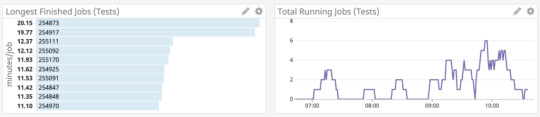
Latency is the total amount of time it takes to service a request. In a CI system, this can be considered to be the total amount of time a build takes to run from start to finish. Latency is better measured on a per-repo or even per-build basis as build length can vary hugely based on the project.

To measure this, we built a small application that queried CircleCI’s API regularly for build lengths, and then shipped over that information to Datadog to allow us to build graphs and visualizations of average build times. This allowed us to chart the results of our improvement experiments empirically and automatically rather than relying on anecdotal or manually curated results as we had done previously.

CircleCI API results

Traffic

Traffic is the amount of demand being placed on your system at any one time. In a CI system, this can be represented by the total number of concurrently running builds.

We were able to measure this by using the same system we built to measure latency metrics. This came in handy when determining the upper and lower bounds for the use of our build resources as it allowed us to see exactly how many jobs were running at any one time.

Errors

Errors are the total amount of requests or calls that fail. In a CI system this can be represented by the total number of builds that fail due to infrastructural reasons. It’s important here to make a distinction between builds that fail correctly, due to tests, linting, code errors, etc. rather than builds that fail due to platform issues.

One issue we encountered was that occasionally AWS would give us “bad” instances when spinning up new builders that would run much slower than a normal “good” instance. Adding error detection into our builder startup scripts allowed us to terminate these and spin up new nodes before they could slow down our running builds.

Saturation

Saturation is how “full” your service is, or how much of your system resources are being used. In a CI system, this is fairly straightforward — how much I/O, CPU, and memory are the builders under load using.

To measure saturation for our setup we were able to tap into cluster metrics by installing a Datadog Agent on each of our builders, which allowed us to get a view into system stats across the cluster.

Datadog job statistics

Identifying the Root Cause

Once your monitoring setup is in place it becomes easier to dig into the root cause of build slowdowns. One of the difficulties in diagnosing CI problems without cluster-wide monitoring is that it can be hard to identify which builders are experiencing load at any one time or how that load affects your builds. Latency monitoring can allow you to figure out which builds are taking the longest, and saturation monitoring can allow you to identify the nodes running those builds for closer investigation.

For us, the new latency measuring we added allowed us to quickly confirm what we had previously guessed: not every build was equal. Some builds ran at the quick speeds we had previously been experiencing but other builds would drag on for far longer than we expected.

In our case this discovery was the big breakthrough — once we could quickly identify builds with increased latency and find the saturated nodes the problem quickly revealed itself: resource contention between starting builds! Due to the large number of tests for our larger builds we use CircleCI’s parallelization feature to split up our tests and run them across the fleet in separate docker containers. Each test container also requires another set of support containers (Redis, MongoDB, etc.) in order to replicate the production environment. Starting all of the necessary containers for each build is a resource-intensive operation, requiring significant amounts of I/O and CPU. Since Nomad uses bin-packing for job distributions our builders would sometimes launch up to 5 different sets of these containers at once, causing massive slow-downs before tests could even start running.

Build Experimentation

Setting up a development environment is key to debugging CI problems once found as it allows you to push your system to its limits while ensuring that none of your testing affects productivity in production. Coinbase maintains a development cluster for CircleCI that we use to test out new versions before pushing them out to production, but in order to investigate our options we turned the cluster into a smaller replica of our production instance, allowing us to effectively load test CircleCI builders. Keeping your development cluster as close as possible to production can help ensure any solutions you find are reflective of what can actually help in a real environment.

Once we had identified why our builds were encountering issues, and we’d set up an environment to run experiments in, we could start developing a solution. We repeatedly ran the same large builds that were causing the problems on our production cluster on different sizes and types of EC2 instances in order to figure out which was the most time and cost-effective options to use.

EC2 instance type comparison

While we previously had been using smaller numbers of large instances to run our builds it turns out the optimal setup for our cluster was actually a very large number of smaller instances (m5.larges in our case) — small enough that CircleCI would only ship one parallelized build container to each instance, preventing the build trampling issues that were the cause of the slow downs. A nice side effect of identifying the correct instance types was that it actually allowed us to reduce our server cost footprint significantly as we were able to size our cluster more closely to its usage.

Problem? Solved!

Applying your changes to a production environment is the final step. Determining whether the effects of the tuning worked can be done the same way the problems were identified — with the four golden signals.

After we had identified what worked best on our development cluster we quickly implemented the new builder sizing in production. The results? A 75% decrease in build time for our largest builds, significant cost savings due to the right-sizing of our cluster, and most important of all: happy developers!

Builds, before and after

This website may contain links to third-party websites or other content for information purposes only (“Third-Party Sites”). The Third-Party Sites are not under the control of Coinbase, Inc., and its affiliates (“Coinbase”), and Coinbase is not responsible for the content of any Third-Party Site, including without limitation any link contained in a Third-Party Site, or any changes or updates to a Third-Party Site. Coinbase is not responsible for webcasting or any other form of transmission received from any Third-Party Site. Coinbase is providing these links to you only as a convenience, and the inclusion of any link does not imply endorsement, approval or recommendation by Coinbase of the site or any association with its operators.

Unless otherwise noted, all images provided herein are by Coinbase.

Continuous Integration at Coinbase: How we optimized CircleCI for speed & cut our build times by… was originally published in The Coinbase Blog on Medium, where people are continuing the conversation by highlighting and responding to this story.

from Money 101 https://blog.coinbase.com/continuous-integration-at-coinbase-how-we-optimized-circleci-for-speed-cut-our-build-times-by-378c8b1d7161?source=rss----c114225aeaf7---4 via http://www.rssmix.com/

[nerdkingdomofficial]

Dev Blog #48: Devotus Tech Update

Happy Friday! Cambo here to kick the weekend off by bringing back the dev tech blogs. We plan to keep them coming at least once a month as we make more progress on development. In regards to the Q&A, most of them are answered and I’ll be sure to post it in our next update blog. For now, here’s our infrastructure dude, Maylyon!

Hey everybody! Maylyon here with a new non-game related, non-engine related, non-tools related tech blog!  Hint: this is your tune-out point if those are the topics you are looking for.  3 . . . 2 . . . 1 . . .  Still here? Excellent!

After literally years of silence about Devotus, I wanted to follow-up with a snapshot of where Devotus is today. If your memory is a little rusty, Devotus will be our mod content distribution pipeline to help mod authors create and manage their home-brewed content and deliver it to end-users.  To get context for this blog entry, you should definitely read those first two blogs.  Without further ado, the "what has been happening?" (aka: "you guys still work on that thing?").

ModJam 2016 ARMAGEDDON!

In case you didn't know, there were mods on Devotus's developmental servers from a TUG v1 ModJam in early 2016.  Don't go rushing to find them now; they're gone.  They were sacrificed to the binary gods in order to make way for…

Going "Serverless"

Suspend your understanding that the term "serverless" is a lie because there are always servers somewhere and play along for a bit.  The old Devotus architecture was built on AWS EBS-backed EC2 instances running a mix of Node.js, C++, and MongoDB.  It looked a little bit like this:

The primary detriments to this approach were:

1.    Paying for these servers (even extremely small servers) when nobody was using them,

2.    Scalability at each layer of the stack would incur even more financial cost and contribute to…

3.    Complexity of the implementation.

 Leveraging AWS API Gateway and AWS Lambda, we have moved to an architecture that looks like:

Moving to this setup allows us to:

1.    Greatly reduce the costs associated with Devotus (especially when nobody is using it),

2.    Offload most of the scalability problem to AWS (less work = more naps),

3.    Synergize our implementation with the other microservices we have been developing on the Infrastructure team.

Support for GitLab

Devotus now allows mod authors to create git repositories on GitLab in addition to GitHub.  It's actually been there for a while but wasn't there in the last blog I wrote. By supporting GitLab and their awesome pricing model, Devotus allows a mod author to choose whether they want their mod's git repository to be public or private at mod creation time.  This choice does not apply to mod's created on GitHub because their pricing model is less awesome (but still pretty awesome) and I'm cheap (see previous section for proof).

Improved Download Metrics

In the "bad old" days (read as "a month ago"), mod download count was just an unsigned integer.  Download request comes in, number gets incremented by one.  Commence spamming download of your own mod to falsely inflate its popularity!  Everybody wins!  . . . Except for the people who want to use the system.

Now, in the "brave new world" days, mod downloads are tracked per-user, per-version.  This allows mod authors to track their mod's popularity throughout its release history and allows end-users to trust that a mod's popularity is probably because of an amazing mod author rather than a mod author's amazing spam-bot.

The Future Is…?

That's all I have for this installment.  I (or somebody from my team) will be back with future Infrastructure updates as we get new and/or exciting things to share.  In the meantime, be sure to jot down all those cool mod ideas you have kicking around in your brain into a little leather-bound notebook so that WHEN TUG v2 is launched and WHEN Devotus is client-facing, you will be ready!

Have a great weekend!

[rabbistevegindi]

MongoDB Replica Set in Docker Swarm Quick Installation Guide

MongoDB Replica Set in Docker Swarm

These scripts Use Docker Swarm with the Community Edition of the official MongoDB container. This MongoDB Replica set can be spread throughout the World. The first script is an AWS Cloudformation that asks a few questions. This creates an EC2 instance which serves as the Docker Swarm Manager.  A Bash scripts launches 3 more instances in regions of your choice,…

[codeonedigest]

AWS EC2 Instance Setup and Run MongoDB in EC2 | Install MongoDB in EC2 S...

Hello friends, a new #video on #awsec2 #server setup #mongodb installation in #ec2 instance is published on #codeonedigest #youtube channel. Learn #aws #ec2 #mongodb #programming #coding with codeonedigest.

 #awsec2 #awsec2instance #awsec2interviewquestionsandanswers #awsec2instancecreation #awsec2deploymenttutorial #awsec2connect #awsec2statuschecks #awsec2project #awsec2full #awsec2createinstance #awsec2interviewquestionsandanswersforfreshers #awsec2instancedeployment #awsec2 #awsec2serialconsole #awsec2consolewindows #awsec2serverrefusedourkey #awsec2serialconsolepassword #awsec2serviceinterviewquestions #awsec2serialconsoleaccess #awsec2serialrefusedourkeyputty #awsec2serverconfiguration #awsec2serialconnect #awsec2 #awsec2instance #awsec2instancecreation #awsec2instanceconnect #awsec2instancedeployment #awsec2instancelinux #awsec2instancelaunch #awsec2instanceconnectnotworking #awsec2instanceinterviewquestions #awsec2instancecreationubuntu #awstutorial #awsec2tutorial #ec2tutorial #mongodbcompass #mongodbinstallation #monogodbtutorial #mongodbtutorialforbeginners #mongodbinaws #mongodbinec2 #awsec2mongodb #mongodbinstallationinaws #mongodbsetupinec2

[nsardo]

Robomongo connect to AWS EC2 behind ssl redirect/tunnel

Robomongo connect to AWS EC2 behind ssl redirect/tunnel

A client of mine has a few EC2 instances that I manage. One of them I installed an SSL Cert on, and all http traffic is forwarded to https.

The Mongodb instance is bound to 0.0.0.0:27017, but I found no way to get Robomongo to connect. Instead, I set up an SSH port forwarding where my local mac listens on port 5555, and passes though (tunnels) the remote server’s port 27017 traffic as a…

[t-baba]

Top 5 PaaS Solutions for Developing Java Applications

Platform as a service (PaaS) is a cloud computing model allowing developers to build and deliver applications over the internet without bothering about the complexity of maintaining the infrastructure usually associated with developing and operating them. Developers can easily access and administer PaaS via a web browser but some have IDE plugins to make using them even simpler.

More elaborately, PaaS is like booking an Uber: You get in and choose your destination and the route you want to get there. How to keep the car running and figuring out the details is up to Uber's driver. Infrastructure as a Service (IaaS), on the other hand, is like renting a car: Driving, fueling (setting it up, maintaining software, etc.), is your job but getting it repaired is someone's else problem.

In case you prefer the IaaS model have a look at this article about the top 5 IaaS solutions for hosting Java applications.

Why use PaaS?

PaaS is a cloud application platform that runs on top of IaaS and host software as a service application. PaaS comprises of operating systems, middleware, servers, storage, runtime, virtualization and other software that allows applications to run in the cloud with many of the system administration abstracted away. This allows organizations to focus on two important things, their customers and their code. PaaS takes care of all the system administration details of setting up servers and VMs, installing runtimes, libraries, middleware, configuring build and testing tools. The workflow in PaaS is as simple as coding in the IDE and then pushing the code using tools like Git and seeing the changes live immediately.

By delivering infrastructure as a service, PaaS also offers the same advantages as IaaS but with additional features of development tools.

Better Coding time: As PaaS provides development tools with pre-coded application components, time to code a new app is reduced.

Dynamic allocation: In today's competitive world, most of the IT teams need to have the flexibility of deploying a new feature or a new service of an application for quick testing or to test these on a small section of clients before making them available to the entire world. With PaaS, such tasks have now become possible.

Develop cross-platform apps easily: PaaS service providers give us various development options for different platforms like computers, mobile devices, and tablets, making cross-platform apps easier and quicker to develop.

Support geographically: It is useful in situations where multiple developers are working on a single project but are not located nearby.

Use helpful tools affordable: Pay-as-you-go method allows you to be charged for what you use. Thus one can use necessary software or analytical tools as per their requirement. It provides support for complete web application lifecycle: building, testing, deploying, managing and updating.

Iaas offers storage and infrastructure resources required to deliver to cloud services whereas organizations using PaaS don’t have to worry about infrastructure nor for services like software updates, storage, operating systems, load balancing, etc. IaaS can be used by organizations which need complete control over their high performing applications, startups and small companies with time & energy constraint, growing organizations which do not want to commit to hardware/software resources, applications which see volatile demands – were scaling up or down is critical based on traffic spikes or valleys.

PaaS for Java is well suited as the JVM, the application server, and deployment archives, i.e., WARs or EARs provide natural isolations for Java applications, allowing many developers to deploy applications in the same infrastructure. As a Java developer, we should keep the following points in mind before choosing a PaaS service:

the flexibility of choosing your application server like JBoss, Tomcat, etc

able to control JVM tuning, i.e., GC tuning

able to plug-in your choice of the stack like MongoDB, MySQL, Redis, etc

the proper logging facility

In this article, we are going compare five PaaS service providers; AWS's Elastic Beanstalk, Heroku, IBM's Bluemix, RedHat's OpenShift and Google App Engine from the view of a Java developer.

Amazon's Elastic Beanstalk

Elastic Beanstalk allows users to create, push and manage web applications in the Amazon Web Services (AWS) console. With Elastic Beanstalk, just upload your code and it automatically handles the deployment, provisioning of a load balancer and the deployment of your WAR file to one or more EC2 instances running the Apache Tomcat application server. Also, you continue to have full control over the AWS resources powering your application.

There is no additional charge for Elastic Beanstalk. It follows Pay-as-you-go model for the AWS resources needed to store and run your applications. Users who are eligible for AWS free usage tier can use it for free.

Here you can get started with Java application on AWS. Once you package your code into a standard Java Web Application Archive (WAR file), you can upload it to Elastic Beanstalk using the AWS Management Console, the AWS Toolkit for Eclipse or any other command line tools. This toolkit is an open source plug-in and offers you to manage AWS resources with your applications and environments from within Eclipse. It has built-in CloudWatch monitoring metrics such as average CPU utilization, request count, and average latency that you can measure once the application is running. Through its Amazon Simple Notification Service, you can receive emails whenever there is any change in the application.

A downside of Elastic Beanstalk can be the lack of clear documentation. There are no release notes, blogs, or forum posts for new stack upgrades.

A Few users of Elastic Beanstalk are Amazon Corporate LLC, RetailMeNot Inc, Vevo LLC, Credible Labs Inc., and Geofeedia Inc..

Heroku

Continue reading %Top 5 PaaS Solutions for Developing Java Applications%

by Ipseeta via SitePoint http://ift.tt/2plC5At

[codeonedigest]

AWS EC2 Instance Setup and Run MongoDB in EC2 | Run MongoDB in EC2 Server

Hello friends, a new #video on #awsec2 #server setup #mongodb installation in #ec2 instance is published on #codeonedigest #youtube channel. Learn #aws #ec2 #mongodb #programming #coding with codeonedigest. #awsec2 #awsec2instance

In this video we will learn amazon EC2 server setup from beginning. Also, install nosql mongo database in EC2 sever. Creating aws linux EC2 instance from AWS management console. Adding firewall rule in the security group to open mongodb port. Login to EC2 instance from local terminal using secret key pair. Download mongo database in EC2 instance. Install Mongo database in EC2…

[globalmediacampaign]

Amazon DocumentDB (with MongoDB compatibility) read autoscaling

Amazon Document DB (with MongoDB compatibility) is a fast, scalable, highly available, and fully managed document database service that supports MongoDB workloads. Its architecture supports up to 15 read replicas, so applications that connect as a replica set can use driver read preference settings to direct reads to replicas for horizontal read scaling. Moreover, as read replicas are added or removed, the drivers adjust to automatically spread the load over the current read replicas, allowing for seamless scaling. Amazon DocumentDB separates storage and compute, so adding and removing read replicas is fast and easy regardless of how much data is stored in the cluster. Unlike other distributed databases, you don’t need to copy data to new read replicas. Although you can use the Amazon DocumentDB console, API, or AWS Command Line Interface (AWS CLI) to add and remove read replicas manually, it’s possible to automatically change the number of read replicas to adapt to changing workloads. In this post, I describe how to use Application Auto Scaling to automatically add or remove read replicas based on cluster load. I also demonstrate how this system works by modifying the load on a cluster and observing how the number of read replicas change. The process includes three steps: Deploy an Amazon DocumentDB cluster and required autoscaling resources. Generate load on the Amazon DocumentDB cluster to trigger a scaling event. Monitor cluster performance as read scaling occurs. Solution overview Application Auto Scaling allows you to automatically scale AWS resources based on the value of an Amazon CloudWatch metric, using an approach called target tracking scaling. Target tracking scaling uses a scaling policy to define which CloudWatch metric to track, and the AWS resource to scale, called the scalable target. When you register a target tracking scaling policy, Application Auto Scaling automatically creates the required CloudWatch metric alarms and manages the scalable target according to the policy definition. The following diagram illustrates this architecture. Application Auto Scaling manages many different AWS services natively, but as of this writing, Amazon DocumentDB is not included among these. However, you can still define an Amazon DocumentDB cluster as a scalable target by creating an Auto Scaling custom resource, which allows our target tracking policy to manage an Amazon DocumentDB cluster’s configuration through a custom HTTP API. This API enables the Application Auto Scaling service to query and modify a resource. The following diagram illustrates this architecture. We create the custom HTTP API with two AWS services: Amazon API Gateway and AWS Lambda. API Gateway provides the HTTP endpoint, and two Lambda functions enable Application Auto Scaling to discover the current number of read replicas, and increase or decrease the number of read replicas. One Lambda function handles the status query (a GET operation), and the other handles adjusting the number of replicas (a PATCH operation). Our complete architecture looks like the following diagram. Required infrastructure Before we try out Amazon DocumentDB read autoscaling, we create an AWS CloudFormation stack that deploys the following infrastructure: An Amazon Virtual Private Cloud (VPC) with two public and two private subnets to host our Amazon DocumentDB cluster and other resources. An Amazon DocumentDB cluster consisting of one write and two read replicas, all of size db.r5.large. A jump host (Amazon Elastic Compute Cloud (Amazon EC2)) that we use to run the load test. It lives in a private subnet and we access it via AWS Systems Manager Session Manager, so we don’t need to manage SSH keys or security groups to connect. The autoscaler, which consists of a REST API backed by two Lambda functions. A preconfigured CloudWatch dashboard with a set of useful charts for monitoring the Amazon DocumentDB write and read replicas. Start by cloning the autoscaler code from its Git repository. Navigate to that directory. Although you can create the stack on the AWS CloudFormation console, I’ve provided a script in the repository to make the creation process easier. Create an Amazon Simple Storage Service (Amazon S3) bucket to hold the CloudFormation templates: aws s3 mb s3:// On the Amazon S3 console, enable versioning for the bucket. We use versions to help distinguish new versions of the Lambda deployment packages. Run a script to create deployment packages for our Lambda functions: ./scripts/zip-lambda.sh Invoke the create.sh script, passing in several parameters. The template prefix is the folder in the S3 bucket where we store the Cloud Formation templates. ./scripts/create.sh For example, see the following code: ./scripts/create.sh cfn PrimaryPassword docdbautoscale us-east-1 The Region should be the same Region in which the S3 bucket was created. If you need to update the stack, pass in –update as the last argument. Now you wait for the stack to create. When the stack is complete, on the AWS CloudFormation console, note the following values on the stack Outputs tab: DBClusterIdentifier DashboardName DbEndpoint DbUser JumpHost VpcId ApiEndpoint When we refer to these later on, they appear in brackets, like Also note your AWS Region and account number. Register the autoscaler: cd scripts python register.py Autoscaler design The autoscaler implements the custom resource scaling pattern from the Application Auto Scaling service. In this pattern, we have a REST API that offers a GET method to obtain the status of the resource we want to scale, and a PATCH method that updates the resource. The GET method The Lambda function that implements the GET method takes an Amazon DocumentDB cluster identifier as input and returns information about the desired and actual number of read replicas. The function first retrieves the current value of the desired replica count, which we store in the Systems Manager Parameter Store: param_name = "DesiredSize-" + cluster_id r = ssm.get_parameter( Name= param_name) desired_count = int(r['Parameter']['Value']) Next, the function queries Amazon DocumentDB for information about the read replicas in the cluster: r = docdb.describe_db_clusters( DBClusterIdentifier=cluster_id) cluster_info = r['DBClusters'][0] readers = [] for member in cluster_info['DBClusterMembers']: member_id = member['DBInstanceIdentifier'] member_type = member['IsClusterWriter'] if member_type == False: readers.append(member_id) It interrogates Amazon DocumentDB for information about the status of each of the replicas. That lets us know if a scaling action is ongoing (a new read replica is creating). See the following code: r = docdb.describe_db_instances(Filters=[{'Name':'db-cluster-id','Values': [cluster_id]}]) instances = r['DBInstances'] desired_count = len(instances) - 1 num_available = 0 num_pending = 0 num_failed = 0 for i in instances: instance_id = i['DBInstanceIdentifier'] if instance_id in readers: instance_status = i['DBInstanceStatus'] if instance_status == 'available': num_available = num_available + 1 if instance_status in ['creating', 'deleting', 'starting', 'stopping']: num_pending = num_pending + 1 if instance_status == 'failed': num_failed = num_failed + 1 Finally, it returns information about the current and desired number of replicas: responseBody = { "actualCapacity": float(num_available), "desiredCapacity": float(desired_count), "dimensionName": cluster_id, "resourceName": cluster_id, "scalableTargetDimensionId": cluster_id, "scalingStatus": scalingStatus, "version": "1.0" } response = { 'statusCode': 200, 'body': json.dumps(responseBody) } return response The PATCH method The Lambda function that handles a PATCH request takes the desired number of read replicas as input: {"desiredCapacity":2.0} The function uses the Amazon DocumentDB Python API to gather information about the current state of the cluster, and if a scaling action is required, it adds or removes a replica. When adding a replica, it uses the same settings as the other replicas in the cluster and lets Amazon DocumentDB choose an Availability Zone automatically. When removing replicas, it chooses the Availability Zone that has the most replicas available. See the following code: # readers variable was initialized earlier to a list of the read # replicas. reader_type and reader_engine were copied from # another replica. desired_count is essentially the same as # desiredCapacity. if scalingStatus == 'Pending': print("Initiating scaling actions on cluster {0} since actual count {1} does not equal desired count {2}".format(cluster_id, str(num_available), str(desired_count))) if num_available < desired_count: num_to_create = desired_count - num_available for idx in range(num_to_create): docdb.create_db_instance( DBInstanceIdentifier=readers[0] + '-' + str(idx) + '-' + str(int(time.time())), DBInstanceClass=reader_type, Engine=reader_engine, DBClusterIdentifier=cluster_id ) else: num_to_remove = num_available - desired_count for idx in range(num_to_remove): # get the AZ with the most replicas az_with_max = max(reader_az_cnt.items(), key=operator.itemgetter(1))[0] LOGGER.info(f"Removing read replica from AZ {az_with_max}, which has {reader_az_cnt[az_with_max]} replicas") # get one of the replicas from that AZ reader_list = reader_az_map[az_with_max] reader_to_delete = reader_list[0] LOGGER.info(f"Removing read replica {reader_to_delete}") docdb.delete_db_instance( DBInstanceIdentifier=reader_to_delete) reader_az_map[az_with_max].remove(reader_to_delete) reader_az_cnt[az_with_max] -= 1 We also store the latest desired replica count in the Parameter Store: r = ssm.put_parameter( Name=param_name, Value=str(desired_count), Type='String', Overwrite=True, AllowedPattern='^d+$' ) Defining the scaling target and scaling policy We use the boto3 API to register the scaling target. The MinCapacity and MaxCapacity are set to 2 and 15 in the scaling target, because we always want at least two read replicas, and 15 is the maximum number of read replicas. The following is the relevant snippet from the registration script: # client is the docdb boto3 client response = client.register_scalable_target( ServiceNamespace='custom-resource', ResourceId='https://' + ApiEndpoint + '.execute-api.' + Region + '.amazonaws.com/prod/scalableTargetDimensions/' + DBClusterIdentifier, ScalableDimension='custom-resource:ResourceType:Property', MinCapacity=2, MaxCapacity=15, RoleARN='arn:aws:iam::' + Account + ':role/aws-service-role/custom-resource.application-autoscaling.amazonaws.com/AWSServiceRoleForApplicationAutoScaling_CustomResource' ) The script also creates the autoscaling policy. There are several important configuration parameters in this policy. I selected CPU utilization on the read replicas as the target metric (CPU utilization is not necessarily the best metric for your workload’s scaling trigger;  other options such as BufferCacheHitRatio may provide better behavior). I set the target value at an artificially low value of 5% to more easily trigger a scaling event (a more realistic value for a production workload is 70–80%). I also set a long cooldown period of 10 minutes for both scale-in and scale-out to avoid having replicas added or removed too frequently. You need to determine the cooldown periods that are most appropriate for your production workload. The following is the relevant snippet from the script: response = client.put_scaling_policy( PolicyName='docdbscalingpolicy', ServiceNamespace='custom-resource', ResourceId='https://' + ApiEndpoint + '.execute-api.' + Region + '.amazonaws.com/prod/scalableTargetDimensions/' + DBClusterIdentifier, ScalableDimension='custom-resource:ResourceType:Property', PolicyType='TargetTrackingScaling', TargetTrackingScalingPolicyConfiguration={ 'TargetValue': 5.0, 'CustomizedMetricSpecification': { 'MetricName': 'CPUUtilization', 'Namespace': 'AWS/DocDB', 'Dimensions': [ { 'Name': 'Role', 'Value': 'READER' }, { 'Name': 'DBClusterIdentifier', 'Value': DBClusterIdentifier } ], 'Statistic': 'Average', 'Unit': 'Percent' }, 'ScaleOutCooldown': 600, 'ScaleInCooldown': 600, 'DisableScaleIn': False } ) Generating load I use the YCSB framework to generate load. Complete the following steps: Connect to the jump host using Session Manager: aws ssm start-session --target Install YCSB: sudo su - ec2-user sudo yum -y install java curl -O --location https://github.com/brianfrankcooper/YCSB/releases/download/0.17.0/ycsb-0.17.0.tar.gz tar xfvz ycsb-0.17.0.tar.gz cd ycsb-0.17.0 Run the load tester. We use workloadb, which is a read-heavy workload: ./bin/ycsb load mongodb -s -P workloads/workloadb -p recordcount=10000000 -p mongodb.url=”mongodb://:@:27017/?replicaSet=rs0&readPreference=secondaryPreferred&retryWrites=false” > load.dat ./bin/ycsb run mongodb -threads 10 -target 100 -s -P workloads/workloadb -p recordcount=10000000 -p mongodb.url=”mongodb://< PrimaryUser>:@:27017/?replicaSet=rs0&readPreference=secondaryPreferred&retryWrites=false” > run.dat These two commands load data in the Amazon DocumentDB database and run a read-heavy workload using that data. Monitoring scaling activity and cluster performance The CloudFormation stack created a CloudWatch dashboard that shows several metrics. The following screenshot shows the dashboard for the writer node. The following screenshot shows the dashboard for the read replicas. As YCSB runs, watch the dashboard to see the load increase. When the CPU load on the readers exceeds our 5% target, the autoscaler should add a read replica. We can verify that by checking the Amazon DocumentDB console and observing the number of instances in the cluster. Cleaning up If you deployed the CloudFormation templates used in this post, consider deleting the stack if you don’t want to keep the resources. Conclusion In this post, I showed you how to use a custom Application Auto Scaling resource to automatically add or remove read replicas to an Amazon DocumentDB cluster, based on a specific performance metric and scaling policy. Before using this approach in a production setting, you should decide which Amazon DocumentDB performance metric best reflects when your workload needs to scale in or scale out, determine the target value for that metric, and settle on a cooldown period that lets you respond to cluster load without adding or removing replicas too frequently. As a baseline, you could try a scaling policy that triggers a scale-up when CPUUtilization is over 70% or FreeableMemory is under 10%. About the Author Randy DeFauw is a principal solutions architect at Amazon Web Services. He works with the AWS customers to provide guidance and technical assistance on database projects, helping them improve the value of their solutions when using AWS. https://aws.amazon.com/blogs/database/amazon-documentdb-with-mongodb-compatibility-read-autoscaling/

[globalmediacampaign]

Getting started with Amazon DocumentDB (with MongoDB compatibility); Part 4 – using Amazon SageMaker notebooks

Many Python developers—and developers in other languages, too—enjoy the developer experience of notebooks, such as Jupyter. They are a useful tool for developing, but also for sharing code, comments, and results in one handy web-based experience. Jupyter and other notebooks have become a common tool, including among machine learning and data science users, which is why it’s no surprise that Amazon SageMaker includes a notebook offering. Python is one of the main languages we see in use with Amazon DocumentDB (with MongoDB compatibility). In this post, we demonstrate how to use Amazon SageMaker notebooks to connect to Amazon DocumentDB for a simple, powerful, and flexible development experience. We walk through the steps using the AWS Management Console, but also include an AWS CloudFormation template to add an Amazon SageMaker notebook to your existing Amazon DocumentDB environment. Solution overview The following diagram illustrates the architecture of our solution’s end state. In the initial state, we have an Amazon DocumentDB cluster deployed in private subnets in an Amazon Virtual Private Cloud (Amazon VPC). Also included in the VPC is a public subnet and a security group that has access to Amazon DocumentDB. This is a common configuration that might also include an Amazon Elastic Compute Cloud (Amazon EC2) machine or an AWS Cloud9 environment, as is described in the Part 1 and Part 2 posts in this series. For instructions on creating your environment, see Setting Up a Document Database. From this starting point, we add an Amazon SageMaker notebook to the public subnet and connect to Amazon DocumentDB. Creating an Amazon SageMaker notebook lifecycle configuration To simplify the environment for our notebook, we use a lifecycle configuration. A lifecycle configuration is a mechanism that can install packages, sample notebooks, or otherwise customize your instance environment. We use the lifecycle configuration mechanism to install the Amazon DocumentDB Python driver pymongo, and to download the CA certificate file for Amazon DocumentDB clusters, which is necessary for connecting using TLS. On the Amazon SageMaker console, under Notebook, choose Lifecycle configurations. Choose Create configuration. For Name, enter a name (such as DocDB-Config). In the Scripts section, on the Start notebook tab, enter the following code: #!/bin/bash sudo -u ec2-user -i <<'EOF' source /home/ec2-user/anaconda3/bin/activate python3 pip install --upgrade pymongo source /home/ec2-user/anaconda3/bin/deactivate cd /home/ec2-user/SageMaker wget https://s3.amazonaws.com/rds-downloads/rds-combined-ca-bundle.pem EOF Choose Create configuration. Creating an Amazon SageMaker notebook instance Now we create the notebook instance itself. On the Amazon SageMaker console, under Notebook, choose Notebook instances. Choose Create notebook instance. For Notebook instance name¸ enter a name (such as DocDB-Notebook). For Notebook instance type, choose your instance type (for this post, choose t2.medium). Under Additional configuration, for Lifecycle configuration, choose the configuration you created (DocDB-Config). For IAM role¸ choose Create a new role. In the Create an IAM role pop-up, select Any S3 bucket. Leave everything else at its default. Choose Create role. Under Network, for VPC, choose the VPC in which your Amazon DocumentDB cluster is. For Subnet, choose a public subnet. For Security group(s), choose a security group that provides access to your Amazon DocumentDB cluster. Choose Create notebook instance. It may take a few minutes to launch this instance. When it’s ready, the instance status shows as InService. Choose Open Jupyter, which opens a new window or tab. Importing the example notebook You can now create a new notebook from the New menu. Amazon SageMaker supports a variety of pre-built environments for your notebook, ranging from basic Python 3 environments to more advanced environments with tools like TensorFlow or Apache Spark dependencies pre-loaded. For this post, import the example Jupyter notebook. Save the file locally. Choose Upload. Choose the local copy of the example notebook. You should see the Getting Started with Amazon DocumentDB notebook listed. Choose Upload to upload the notebook file to Amazon SageMaker. Choose Getting Started with Amazon DocumentDB and Amazon SageMaker Notebook.ipynb to open the notebook. This sample notebook demonstrates a few simple operations: Import some needed packages Gather the connection details and credentials for the Amazon DocumentDB cluster and make the connection Issue a basic command to verify a successful connection Issue some insert statements Issue some read statements You can run the notebook cell by cell and provide the Amazon DocumentDB information when prompted. Terminal access For those of you who like to use command-line tools or have additional tools beyond Python, Amazon SageMaker notebook instances can also open a terminal session. On the Jupyter main page, from the New menu, choose Terminal. This opens a new tab in your browser with a terminal session. This provides terminal access to the Amazon SageMaker instance that you created. You could, for example, install utilities like mongoimport for bulk loading of data. Cleaning up If you used the CloudFormation template, you should be able to delete the stack, which deletes the Amazon SageMaker notebook instance and the Amazon SageMaker lifecycle configuration, as well as the IAM role used to run the notebook instance. If you performed these steps manually, you need to use the AWS console to remove the following components: Notebook instance Lifecycle configuration IAM role we created when making the notebook instance Summary In this post, we demonstrated how to connect an Amazon SageMaker notebook instance to Amazon DocumentDB, thereby bringing this powerful development environment together with the power of Amazon DocumentDB. For more information, see Ramping up on Amazon DocumentDB (with MongoDB compatibility). For more information about recent launches and blog posts, see Amazon DocumentDB (with MongoDB compatibility) resources. About the Author Brian Hess is a Senior Solution Architect Specialist for Amazon DocumentDB (with MongoDB compatibility) at AWS. He has been in the data and analytics space for over 20 years and has extensive experience with relational and NoSQL databases. https://aws.amazon.com/blogs/database/getting-started-with-amazon-documentdb-with-mongodb-compatibility-part-4-using-amazon-sagemaker-notebooks/

[globalmediacampaign]

Migrating relational databases to Amazon DocumentDB (with MongoDB compatibility)

Relational databases have been the foundation of enterprise data management for over 30 years. But the way we build and run applications today, coupled with unrelenting growth in new data sources and growing user loads, is pushing relational databases beyond their limits. This can inhibit business agility, limit scalability, and strain budgets, compelling more and more organizations to migrate to alternatives like NoSQL databases. Amazon DocumentDB (with MongoDB compatibility) is a fast, scalable, highly available, and fully managed document database service that supports MongoDB workloads. As a document database, Amazon DocumentDB makes it easy to store, query, and index JSON data. To get started with Amazon DocumentDB, see Getting Started with Amazon DocumentDB (with MongoDB compatibility). If your data is stored in existing relational databases, converting relational data structures to documents can be complex and involve constructing and managing custom extract, transform, and load (ETL) pipelines. Amazon Database Migration Service (AWS DMS) can manage the migration process efficiently and repeatably. With AWS DMS, you can perform minimal downtime migrations, and can replicate ongoing changes to keep sources and targets in sync. This post provides an overview on how you can migrate your relational databases like MySQL, PostgreSQL, Oracle, Microsoft SQL Server, and others to Amazon DocumentDB using AWS DMS. Data modeling Before addressing the mechanics of using AWS DMS to copy data from a relational database to Amazon DocumentDB, it’s important to understand the basic differences between relational databases and document databases. Relational databases Traditional relational database management system (RDBMS) platforms store data in a normalized relational structure and use structured query language (SQL) for database access. This reduces hierarchical data structures to a set of common elements that are stored across multiple tables. The following diagram provides an overview of the structure of the Employees sample database. This image was taken from MySQL’s employees sample database under the Creative Commons Attribution-ShareAlike license. No changes have been made. When developers need to access data in an application, you merge data from multiple tables together in a process called as join. You predefine your database schema and set up rules to govern the relationships between fields or columns in your tables. RDBMS platforms use an ad hoc query language (generally a type of SQL) to generate or materialize views of the normalized data to support application-layer access patterns. For example, to generate a list of departments with architects (sorted by hire date), you could issue the following query against the preceding schema: SELECT * FROM departments INNER JOIN dept_emp ON departments.dept_no = dept_emp.dept_no INNER JOIN employees ON employees.emp_no = dept_emp.emp_no INNER JOIN titles ON titles.emp_no = employees.emp_no WHERE titles.title IN (‘Architect’) ORDER BY employees.hire_date DESC; The preceding query initiates complex queries across a number of tables and then sorts and integrates the resulting data. One-time queries of this kind provide a flexible API for accessing data, but they require a significant amount of processing. If you’re running multiple complex queries, there can be considerable performance impact, leading to poor end-user experience. In addition, RDBMSs require up-front schema definition, and changing the schema later is very expensive. You may have use cases in which it’s very difficult to anticipate the schema of all the data that your business will eventually need. Therefore, RDBMS backends may not be appropriate for applications that work with a variety of data. However, NoSQL databases (like document databases) have dynamic schemas for unstructured data, and you can store data in many ways. They can be column-oriented, document-oriented, graph-based, or organized as a key-value store. This flexibility means that: You can create documents without having to first define their structure Each document can have its own unique structure The syntax can vary from database to database You can add fields as you go For more information, see What is NoSQL? Document databases Amazon DocumentDB is a fully managed document database service that makes it easy to store, query, and index JSON data. For more information, see What is a Document Database? and Understanding Documents. The following table compares terminology used by document databases with terminology used by SQL databases. SQL Amazon DocumentDB Table Collection Row Document Column Field Primary key ObjectId Index Index View View Nested table or object Embedded document Array Array Using Amazon DocumentDB, you can store semi-structured data as a document rather than normalizing data across multiple tables, each with a unique and fixed structure, as in a relational database. Fields can vary from document to document—you don’t need to declare the structure of documents to the system, because documents are self-describing. Development is simplified because documents map naturally to modern, object-oriented programming languages. The following is an example of a simple document. In the following document, the fields SSN, LName, FName, DOB, Street, City, State-Province, PostalCode, and Country are all siblings within the document: { "SSN": "123-45-6789", "LName": "Rivera", "FName": "Martha", "DOB": "1992-11-16", "Street": "125 Main St.", "City": "Anytown", "State-Province": "WA", "PostalCode": "98117", "Country": "USA" } For more information about adding, querying, updating, and deleting documents, see Working with Documents. Amazon DocumentDB is designed to work with your existing MongoDB applications and tools. Be sure to use drivers intended for MongoDB 3.4 or newer. Internally, Amazon DocumentDB implements the MongoDB API by emulating the responses that a MongoDB client expects from a MongoDB server. Therefore, you can use MongoDB APIs to query your Amazon DocumentDB database. For example, the following query returns all documents where the Item field is equal to Pen: db.example.find( { "Item": "Pen" } ).pretty() For more information about writing queries for Amazon DocumentDB, see Querying. Let’s say that you have a table in your relational database called Posts and another table called Comments, and the two are related because each post has multiple comments. The following is an example of the Posts table. post_id title 1 Post 1 2 Post 2 The following is an example of the Comments table. comment_id post_id author comment 1 1 Alejandro Rosalez Nice Post 2 1 Carlos Salazar Good Content 3 2 John Doe Improvement Needed in the post In order to get the comments of a post with title “Post 1”, you will need to execute an expensive JOIN query similar to below: SELECT author, comment FROM Comments INNER JOIN Posts ON Comments.post_id = Posts.post_id WHERE Posts.title LIKE “Post 1"; While modelling data for documents, you can create one collection of documents that represents a post with an array of comments. See the following output: { "_id" : NumberLong(1), "title" : "Post 1", "comments" : [ { "author" : "Alejandro Rosalez", "content" : " Nice Post" }, { "author" : "Carlos Salazar", "content" : " Good Content" } ] } { "_id" : NumberLong(2), "title" : "Post 2", "comments" : [ { "author" : "John Doe", "content" : " Improvement Needed in the post" } ] } The following query will provide the comments for the post with title as “Post 1”: rs0:PRIMARY> db.posts.find({ “title”: “Post 1” }, {“comments”: 1, _id: 0}) { “comments” : [ { “author” : “Alejandro Rosalez”, “content” : ” Nice Post” }, { “author” : “Carlos Salazar”, “content” : ” Good Content” } ] } For more information about data modeling, see Data Modeling Introduction. Solution overview You can use AWS DMS to migrate (or replicate) data from relational engines like Oracle, Microsoft SQL Server, Azure SQL Database, SAP ASE, PostgreSQL, MySQL and others to an Amazon DocumentDB database. You can also migrate the data from non-relational sources, but those are beyond the scope of this post. As depicted in the following architecture, you deploy AWS DMS via a replication instance within your Amazon Virtual Private Cloud (Amazon VPC). You then create endpoints that the replication instance uses to connect to your source and target databases. The source database can be on premises or hosted in the cloud. In this post, we create the source database in the same VPC as the target Amazon DocumentDB cluster. AWS DMS migrates data, tables, and primary keys to the target database. All other database elements are not migrated. This is because AWS DMS takes a minimalist approach and creates only those objects required to efficiently migrate the data. The following diagram shows the architecture of this solution. The walkthrough includes the following steps: Set up the source MySQL database. Set up the target Amazon DocumentDB database. Create the AWS DMS replication instance. Create the target AWS DMS endpoint (Amazon DocumentDB). Create the source AWS DMS endpoint (MySQL). Create the replication task. Start the replication task. Clean up your resources. As a pre-requisite, we just need an AWS Account and an IAM user which has appropriate access permissions. This walkthrough incurs standard service charges. For more information, see the following pricing pages: AWS Database Migration Service pricing Amazon DocumentDB (with MongoDB compatibility) pricing Amazon EC2 pricing Setting up the source MySQL database We first launch an Amazon Linux 2 EC2 instance and install MySQL server. For instructions, see Installing MySQL on Linux Using the MySQL Yum Repository. Then, we load the sample Employee database with the structure as shown in the beginning of the post. We used the following commands to load the sample database: git clone https://github.com/datacharmer/test_db.git cd test_db mysql -u root -p -t < employees.sql Setting up the target Amazon DocumentDB database For instructions on creating a new Amazon DocumentDB cluster and trying out some sample queries, see Setting up an Document Database. For this walkthrough, we create the cluster my-docdb-cluster with one instance my-docdb-instance. The following screenshot shows the cluster details. Creating an AWS DMS replication instance AWS DMS uses an Amazon Elastic Compute Cloud (Amazon EC2) instance to perform the data conversions as part of a given migration workflow. This EC2 instance is referred to as the replication instance. A replication instance is deployed within a VPC, and it must have access to the source and target databases. It’s a best practice to deploy the replication instance into the same VPC where your Amazon DocumentDB cluster is deployed. You also need to make other considerations in terms of sizing your replication instance. For more information, see Choosing the optimum size for a replication instance. To deploy a replication instance, complete the following steps: Sign in to the AWS DMS console within the AWS account and Region where your Amazon DocumentDB cluster is located. In the navigation pane, under Resource management, choose Replication instances. Choose Create replication instance. This brings you to the Create replication instance page. For Name, enter a name for your instance. For this walkthrough, we enter mysql-to-docdb-dms-instance. For Description, enter a short description. For Instance class, choose your preferred instance. For this walkthrough, we use a c4.xlarge instance. Charges may vary depending on your instance size, storage requirements, and certain data transfer usage. For more information, see AWS Database Migration Service Pricing. For Engine version, choose your AWS DMS version (prefer the latest stable version – not the beta versions). Select Publicly accessible option, if you want your instance to be publicly accessible. If you’re migrating from a source that exists outside of your VPC, you need to select this option. If the source database is within your VPC, accessible over an AWS Direct Connect connection, or via a VPN tunnel to the VPC, then you can leave this option unselected. In the Advanced security and network configuration section, select your suitable Security Group (that allows network traffic access to the source and target database). You can also define other options, such as specific subnets, Availability Zones, custom security groups, and if you want to use AWS Key Management Service (AWS KMS) encryption keys. For more information, see Working with an AWS DMS replication instance. For this post, we leave the remaining options at their defaults. Choose Create. For more details and screenshots, see Create a replication instance using the AWS DMS console. Provisioning your replication instance may take a few minutes. Wait until provisioning is complete before proceeding to the next steps. Creating a target AWS DMS endpoint After you provision a replication instance, you define the source and targets for migrating data. First, we define the connection to our target Amazon DocumentDB cluster. We do this by providing AWS DMS with a target endpoint configuration. On the AWS DMS console, under Resource management, choose Endpoints. Choose Create endpoint. This brings you to the Create endpoint page. For Endpoint type, select Target endpoint. For Endpoint Identifier, enter a name for your endpoint. For this walkthrough, we enter target-docdb-cluster For Target Engine, select docdb For Server name, enter the cluster endpoint for your target Amazon DocumentDB cluster (available in the Amazon DocumentDB cluster details on the Amazon DocumentDB console). To find the cluster endpoint of your Amazon DocumentDB cluster, refer to Finding a Cluster’s Endpoint. For Port, enter the port you use to connect to Amazon DocumentDB (the default is 27017). For SSL mode, choose verify-full. For CA certificate, do one of the following to attach the SSL certificate to your endpoint: If available, choose the existing rds-combined-ca-bundle certificate from the Choose a certificate drop-down menu. Download the new CA certificate bundle. This operation downloads a file named rds-combined-ca-bundle.pem. Then complete the following: In the AWS DMS endpoint page, choose Add new CA certificate. For Certificate identifier, enter rds-combined-ca-bundle. For Import certificate file, choose Choose file and navigate to the rds-combined-ca-bundle.pem file that you previously downloaded. Open the file and choose Import certificate. Choose rds-combined-ca-bundle from the Choose a certificate drop-down menu. For User name, enter the master user name of your Amazon DocumentDB cluster. For this walkthrough, we enter masteruser For Password, enter the master password of your Amazon DocumentDB cluster. For Database name, enter suitable value. For this walkthrough, we enter employees-docdb as the database name. In the Test endpoint connection section, ensure that your endpoint is successfully connected. This can be confirmed when status shows as successful as seen in the following screenshot. For more information on this step, see Creating source and target endpoints. Creating the source AWS DMS endpoint We now define the source endpoint for your source RDBMS. On the AWS DMS console, under Resource management, choose Endpoints. Choose Create endpoint. For Endpoint type¸ select Source endpoint. For Endpoint Identifier, enter a name. For this walkthrough, we enter source-ec2-mysql For Source engine, choose your source database engine. For this walkthrough, we used mysql. For Server name, enter your source endpoint. This can be the IP or DNS address of your source machine For Port, enter the DB port on the source machine (here 3306). For Secure Socket Layer, choose the value depending on user configurations set in your source mysql database. For this walkthrough, we used none. For User name, enter the user name of your source DB. For this walkthrough, we enter mysqluser. For Password, enter the master password of your source DB. For Database name, enter suitable value. For this walkthrough, we enter employees. In the Test endpoint connection section, ensure that your endpoint is successfully connected. This can be confirmed when status shows as successful as seen in the following screenshot. For more information on this step, see Creating source and target endpoints. Creating a replication task After you create the replication instance and source and target endpoints, you can define the replication task. For more information, see Creating a task. On the AWS DMS console, under Conversion & Migration, choose Database migration tasks. Choose Create database migration task. For Task identifier, enter your identifier. For this walkthrough, we enter dms-mysql-to-docDB Choose your replication instance and source and target database endpoints. For this walkthrough, we enter mysql-to-docdb-dms-instance, source-ec2-mysql and target-docdb-cluster Choose the Migration Type as per your requirements: Migrate existing data – This will migrate the existing data from source to target. This will not replicate the ongoing changes on the source. Migrate existing data and replicate ongoing changes – This will migrate the existing data from source to target and will also replicate changes on the source database that occur while the data is being migrated from the source to the target. Replicate data changes only – This will only replicate the changes on the source database and will not migrate the existing data from source to target. You may refer to Creating a task for more details on this option. For this walkthrough, we enter Migrate existing data. On the Task settings page, select Wizard as the Editing Mode. On the Task settings page, you can select Target table preparation mode. You can choose one of the following, depending on your requirements: Do nothing – This creates the table if a table isn’t on the target. If a table exists, this leaves the data and metadata unchanged. AWS DMS can create the target schema based on the default AWS DMS mapping of the data types. However, if you wish to pre-create the schema (or have a different data type) on the target database (Amazon DocumentDB), you can choose to create the schema and use this mode to perform the migration of data to your desired schema. You can also use mapping rules and transformation rules to support such use cases. Drop tables on target – This drops the table at the target and recreates the table. Truncate – This truncates the data and leaves the table and metadata intact. For this walkthrough, we enter Drop tables on target. On the Task settings page, you will have the option to select Include LOB columns in replication. For this walkthrough, we used Limited LOB mode with Max LOB size (KB) as 32. You can choose one of the following depending on your requirements: Don’t include LOB columns – LOB columns are excluded from the migration. Full LOB mode – Migrate complete LOBs regardless of size. AWS DMS migrates LOBs piecewise in chunks controlled by the Max LOB size parameter. This mode is slower than using Limited LOB mode. Limited LOB mode – Truncate LOBs to the value of the Max LOB size parameter. This mode is faster than using Full LOB mode. For this walkthrough, we unchecked Enable validations. AWS DMS provides support for data validation to ensure that your data was migrated accurately from the source to the target. This may slow down the migration. Refer to AWS DMS data validation for more details. On the Task settings page, select Enable CloudWatch logs. Amazon CloudWatch logs are useful if you encounter any issues when the replication task runs. You also need to provide IAM permissions for CloudWatch to write AWS DMS logs. Choose your values for Source Unload, Task Manager¸ Target Apply, Target Load, and Source Capture. For this walkthrough, we used Default. Initially, you may wish to keep the default values for logging levels. if you encounter problems, you can modify the task to select more detailed logging information that can help you to troubleshoot. To read more, refer to Logging task settings and How do I enable, access, and delete CloudWatch logs for AWS DMS? The Table Mapping configuration section of the replication task definition specifies the tables and columns that AWS DMS migrates from source MySQL database to Amazon DocumentDB. You can specify the required information two different ways: using a Guided UI or a JSON editor. For more information about sophisticated selection, filtering and transformation possibilities, including table and view selection and using wildcards to select schemas, tables, and columns, see Using table mapping to specify task settings. For this walkthrough, we used the following values: Editing mode – Wizard Schema – Enter a schema Schema name – employees Table name – % Action – Include Refer to Specifying table selection and transformations rules from the console for screenshots of this step. Choose Create task. Starting the replication task The definition of the replication task is now complete and you can start the task. The task status updates automatically as the process continues. For this post, we configured migration type as Migrate existing data, so the status of the task shows as Load Complete, which may differ depending on the migration type. If an error occurs, the error appears on the Overview details tab (see the following screenshot) under Last failure message. For more information about troubleshooting, see Troubleshooting migration tasks in AWS Database Migration Service. For our sample database, the AWS DMS process takes only a few minutes from start to finish. For more information about connecting to your cluster, see Developing with Amazon DocumentDB. For this post, we use the mongo shell to connect to the cluster. If you connect to the target cluster, you can observe the migrated data. The following query lists all the databases in the cluster: rs0:PRIMARY> show dbs; employees-docdb 1.095GB The following query switches to use the employees-docdb database: rs0:PRIMARY> use employees-docdb; switched to db employees-docdb The following query lists all the collections in the employees-docdb database: rs0:PRIMARY> db.getCollectionNames() [ "departments", "dept_emp", "dept_manager", "employees", "salaries", "titles" The following query selects one document from the departments collection: rs0:PRIMARY> db.departments.findOne() { "_id" : { "dept_no" : "d009" }, "dept_no" : "d009", "dept_name" : "Customer Service" } The following query selects one document from the employees collection: rs0:PRIMARY> db.employees.findOne() { "_id" : { "emp_no" : 10001 }, "emp_no" : 10001, "birth_date" : ISODate("1970-09-22T11:20:56.988Z"), "first_name" : "Georgi", "last_name" : "Facello", "gender" : "M", "hire_date" : ISODate("1986-06-26T00:00:00Z") } The following query counts the number of documents in the employees collection: rs0:PRIMARY> db.employees.count() 300024 Cleaning up When database migration is complete, you may wish to delete your AWS DMS resources. On the AWS DMS dashboard, choose Tasks in the navigation pane. Locate the migration task that you created earlier and click on drop-down Actions button and choose Delete. In the navigation pane, choose Endpoints. Choose the source and target endpoints that you created earlier and click on drop-down Actions button and choose Delete. In the navigation pane, choose Replication instances. Choose the replication instance that you created earlier and click on drop-down Actions button and choose Delete. Summary AWS DMS can quickly get you started with Amazon DocumentDB and your own data. This post discussed how to migrate a relational database to Amazon DocumentDB. We used an example MySQL database and migrated a sample database to Amazon DocumentDB. You can use similar steps for migration from a different supported RDBMS engine to Amazon DocumentDB. To learn more about Amazon DocumentDB, see What Is Amazon DocumentDB (with MongoDB Compatibility). To learn more about AWS DMS, see Sources for AWS Database Migration Service and Using Amazon DocumentDB as a target for AWS Database Migration Service. About the Author Ganesh Sawhney is a Partner Solutions Architect with the Emerging Partners team at Amazon Web Services. He works with the India & SAARC partners to provide guidance on enterprise cloud adoption and migration, along with building AWS practice through the implementation of well architected, repeatable patterns and solutions that drive customer innovation. Being an AWS Database Subject Matter Expert, he has also worked with multiple customers for their database and data warehouse migrations. https://aws.amazon.com/blogs/database/migrating-relational-databases-to-amazon-documentdb-with-mongodb-compatibility/