#excel eomonth

[eyescananalyze]

EXCEL - Formulas and Functions - Date and Time - eomonth #viralvideo #vi...

[fmskillsharing]

#excelfunctions #exceltips #sumif #iffunction #nestedif #uniquefunction #filterfunction #lookupfunction #vlookup #hlookup #fuzzylookup #sortfunction #dateandtimefunction #roundfunction #subtotalfunction #dmax #dmin #leftfunction #rightfunction #midfunction #findfunction #eomonth #upperfunction #lowerfunction #properfunction #trimfunction #edate #maxfunction #minfunction #largefunction #smallfunction #frequencyfunction

[techguruplus]

How to Sum in Date Range in Excel Sumifs Formula & EOmonth Formula

Tutorial Video Download Excel File More Excel Projects

[makecareersolution]

15 Advanced Excel Formulas You Must Know

Introduction

Microsoft Excel is a powerful tool for data analysis and management. It is used by businesses and individuals worldwide to organize and analyze data, create charts and graphs, and automate tasks. Excel offers a wide range of built-in functions, but advanced Excel formulas take your skills to the next level.

VLOOKUP

VLOOKUP is one of the most commonly used Excel formulas. It is used to find and retrieve data from a specific column in a table. It works by matching a lookup value to a corresponding value in the first column of a table and returning a value in the same row from a specified column.

INDEX-MATCH

INDEX-MATCH is an alternative to VLOOKUP. It is used to find and retrieve data from a specific row or column in a table. It works by matching a lookup value to a corresponding value in a specified column or row and returning a value from a specified row or column.

SUMIFS

SUMIFS is used to sum values in a range that meet multiple criteria. It works by specifying the range to sum, as well as the criteria to be met for each corresponding cell in a separate range.

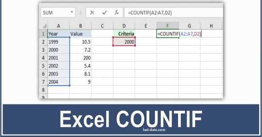
COUNTIFS

COUNTIFS is used to count the number of cells in a range that meet multiple criteria. It works by specifying the range to count, as well as the criteria to be met for each corresponding cell in a separate range.

IFERROR

IFERROR is used to replace an error value with a specific value or message. It works by testing a formula for an error value and returning a specified value if an error is detected.

CONCATENATE

CONCATENATE

 is used to join two or more text strings into a single string. It works by specifying the text strings to be joined and the separator to be used between them.

LEFT, RIGHT, and MID

LEFT, RIGHT, and MID are used to extract a specific number of characters from a text string. LEFT is used to extract characters from the beginning of a string, RIGHT is used to extract characters from the end of a string, and MID is used to extract characters from the middle of a string.

LEN

LEN is used to determine the length of a text string. It works by counting the number of characters in a string.

TRIM

TRIM is used to remove extra spaces from a text string. It works by removing all leading and trailing spaces, as well as any extra spaces between words.

SUBSTITUTE

SUBSTITUTE is used to replace a specific text string within a larger text string with a different text string. It works by specifying the text string to be replaced, the text string to replace it with, and the text string in which the replacement is to occur.

NETWORKDAYS

NETWORKDAYS is used to calculate the number of working days between two dates. It works by excluding weekends and specified holidays from the calculation.

EOMONTH

EOMONTH is used to calculate the last day of the month based on a specified date. It works by adding a specified

If you are looking to enhance your Excel skills, then learning advanced Excel formulas is the next step for you. Knowing advanced Excel formulas will help you automate complex calculations, save time, and improve your overall productivity. In this Blog, we have discussed 15 advanced Excel formulas that you must know.

[gerrinson]

Oh, yeah. Sorry. Moose out front should've told you. Excel formulae are a great insight into how someone's mind works. Somewhat. It definitely usually tells you if they are trained at coding logic.

I failed a 'test' for a job interview process. They wanted me to program it to fill out the first and last days of each month as part of the dataset reporting. So, being myself, I used the EOMONTH formula to pull the last day. Quick, easy, clean. And, according to the employer, a failure. Because they explicitly wanted to test my ability to use nested ifs. Like, my dudes, maybe put it in the directions if that's what you want. So A) they didn't understand there was an easier way than nested ifs and B) they failed me for being too efficient. Probably dodged a bullet not getting that job.

okay never mind i DO want push notifications for “exciting updates” from businesses because i just learned that excel delivered the xlookup function unto the starving masses FIVE YEARS AGO. general release MARCH 2020. are you kidding me. are you kidding me!!! it took until 2025 for me to make a typo in the formula bar and go oh hello? what’s this? and change my entire life. not only have i been dealing with a global pandemic i have been doing it WHILE indexing and matching and nesting iserror vlookups i am going! to! walk into the sea!!!

[1lastdate]

COUNTIFS Function in Excel Hindi

COUNTIFS Function in Excel Hindi

Excel में COUNTIFS Function एक ऐसा Function है जिसके द्वारा multiple criteria के आधार पर हम Data Range में Sales को Count कर सकते है। इसे Excel में Statistical Functions के अंतर्गत रखा गया है। यह Function COUNTIF function की तरह ही काम करता है। दोनों में अंतर बस इतना है कि COUNTIF में सिर्फ एक criteria ही Define कर सकते है जबकि COUNTIFS function में हम multiple criteria का Use कर सकते है। इस Post…

[evaninocom]

How to use EOMONTH() to return the last day of the month and more in Excel

How to use EOMONTH() to return the last day of the month and more in Excel

There’s more to EOMONTH() in Microsoft Excel than the last day of the month. Learn how to put it to use in your spreadsheets. Image: Rawpixel/iStockphoto Dates play a part in many spreadsheets, but they can be a bit mysterious, especially when Excel doesn’t offer a date function that returns exactly the value you need. Fortunately, the more you know, the easier dates are to work with. In this…

[globalteachonline]

What you'll learn Learn functions & formulas with the easiest & the most comprehensible examples.Learn to prepare for the most Excel practical examinations.Learn to master usage of Excel in an office environment.Learn various charts & Pivot Table with the easiest examples.Learn practically MS Excel from basic to advance.Learn unique & difficult combination of different functions in Excel.Students who want to learn Excel. Professionals who want to improve in Excel & bring more clarity to various options.This course contains the basics to advance the learning of Excel. The quick explanation technique in video saves a lot of time, it has various functions & formulas explained in the easiest, most accurate & most comprehensible examples for all. This course explains what are rows & columns how to hide/unhide & delete them, cell & range of cells & how to drag cells, how many spreadsheets in one Excel workbook, different Tabs & Ribbons, what is the Quick Access Toolbar, Name Box & Formula Bar, how to navigate Excel & how to save & save As. The application of BODMAS in Excel, learn when it will be applicable & when not. In this course, you will get to learn the basics & advanced usage of functions like LEFT, RIGHT, MID, CONCATENATE, NOW, TODAY, EOMONTH, NETWORKDAYS, NETWORKDAYSINTL, WORKDAY, SUBTOTAL, MOD & QUOTIENT, IFERROR, List of Errors & Various Error Alerts, LOOKUP, HLOOKUP, HLOOKUP, SUMPRODUCT, SUM(Array)VLOOKUP, PMT, PPMT, IPMT, FV, NPV & IRR, XNPV & XIRR, SUM, AVERAGE, MIN, MAX, COUNT, IF, IF AND, IF OR, IF NOT, NESTED IF, INDEX & MATCH with Vlookup, MAX, Array (Ctrl + Shift + Enter) & many more with a combination of two or more functions. This course will explain variously charts available in Excel, it also explains the distinction between normal table/chart & Pivot table/chart. The explanation of various shortcuts available in Excel will speed up our day to day work. I am looking forward to you, subscribing to the course.Who this course is for:This course is designed for the beginner, intermediate & advanced users of Excel.This course is best for students wanting to practically learn Excel.This course is best for professionals wanting to bring more clarity in Excel & learn new methods.This course can help various business owners & employees to get hands-on Excel.Beginner

[congduc-1612]

Sử dụng hàm EOMONTH – Trả về ngày cuối cùng của tháng trong Excel

Khi nhắc đến các hàm ngày tháng hay thời gian, chắc hẳn bạn đã được nghe đến hàm EOMONTH, đây là một hàm khá đơn giản trong Excel. Hàm này sẽ giúp bạn tính toán và trả về kết quả là ngày cuối cùng của một tháng bạn muốn tìm trong Excel. Bài viết hôm nay Azgad sẽ hướng dẫn bạn cách thực hiện của hàm EOMONTH này qua ví dụ minh họa cụ thể. Cùng theo dõi và thực hành với Azgad để hiểu rõ hơn nhé!

Hàm EOMONTH

Hàm EOMONTH  khá đơn giản và là sự lựa chọn tốt ưu cho người sử dụng Excel. Hàm này sẽ giúp người dùng tính toán và trả về kết quả của ngày cuối cùng cho một tháng cụ thể trong Excel.

Công thức hàm EOMONTH

Cấu trúc hàm

=EOMONTH(Start_date, Months)

Giải thích hàm:

Start_date (bắt buộc phải có): Ngày tháng được hiển thị dùng xác định ngày cuối cùng của tháng đó hoặc tháng trước và tháng sau.

Months (tham số bắt buộc phải có): Số tháng để xác định ngày cuối cùng cho tháng. Với Months > 0 thì kết quả sẽ hiển thị ngày mới trong tương lai. Ngược lại, Months < 0 thì hàm sẽ hiển thị kết quả là một ngày mới trong quá khứ.

Lưu ý khi dùng:

Hàm Excel sẽ lưu trữ ngày tháng ở dạng số seri để quá trình tính toán được diễn ra thuận lợi.

Nếu bạn nhập giá trị Start_date là một ngày không hợp lệ thì hàm Excel sẽ báo về kết quả là giá trị lỗi #VALUE!.

Khi giá trị Start_date cộng với giá trị Months tạo ra một ngày không hợp lệ thì hàm Excel sẽ báo lỗi kết quả là #NUM!.

Hàm CEILING trong Excel

Hàm CEILING

Hàm CEILING là hàm dùng để làm tròn một số bất kỳ trong bảng tính Excel đến một bội số gần nhất một cách rất đơn giản.

Bội số được hiểu là số chia hết cho chính nó.

Bội số gần nhất được hiểu là một số do chính bạn quyết định, được thêm vào để tìm một kết quả gần với giá trị ban đầu nhất.

Cấu trúc hàm CEILING

=CEILING(Number, Significance)

Trong đó:

Number: Giá trị cần để làm tròn đến bội số.

Significance: Giá trị bội số cần làm tròn đến.

Lưu ý:

Tham số không phải số thì hàm trả về giá trị lỗi là #VALUE!.

Number] và [Significance] đều là số âm thì kết quả cuối cùng sẽ được làm tròn xuống.

[Number] là số âm và [Significance] là số dương thì kết quả cuối cùng sẽ được làm tròn lên và về gần.

Hàm FIND trong Excel

Hàm FIND là gì?

Hàm FIND là hàm dò tìm kiếm một chuỗi ký tự trong văn bản được cho trước. Hàm Excel này sẽ tự động tìm kiếm và trả về vị trí tương ứng với ký tự cần tìm.

Công thức hàm FIND

=FIND (find_text; within_text; [start_num])

Trong đó:

find_text: Ký tự hoặc văn bản cần tìm kiếm.

within_text: Chuỗi văn bản chứa giá trị cần tìm kiếm vị trí của ký tự.

[start_num]: Vị trí bắt đầu tìm kiếm ký tự được yêu cầu.

Bài viết trên Azgad đã hướng dẫn bạn rất chi tiết về cách dùng hàm EOMONTH và có ví dụ cụ thể khi làm việc với hàm Excel này. Azgad hy vọng bạn sẽ hoàn thành tốt mọi công việc và nâng cao hiệu suất làm việc. Nhớ theo dõi Azgad hằng ngày để nhận thêm nhiều kiến thức hay và hữu ích cho công việc của bạn.

[exceltricks]

Excel: englische Funktion auf Deutsch eingeben — PC-Hilfe und Support von PC-Meister

Excel: englische Funktion auf Deutsch eingeben — PC-Hilfe und Support von PC-Meister

Tipps & Tricks Excel: englische Funktion auf Deutsch eingeben Englische Excel-Formeln haben ein Komma statt eines Strichpunkts und heissen anders, z.B. EOMONTH statt MONATSENDE. Hier übersetzen Sie es. © Bild & Inhalt: Autor: → WeiterlesenExcel: englische Funktion auf Deutsch eingeben — PC-Hilfe und Support von PC-Meister

[excel10tutorial]

How To Use Eomonth Function In Excel

[1lastdate]

COUNTIF Function in Excel | Use of COUNTIF in Excel

COUNTIF Function in Excel | Use of COUNTIF in Excel

Excel में COUNTIF Function को statistical function की category में रखा गया है। यह Function किसी perticular criteria के आधार पर Data Range में cells को count करने के लिए Use किया जाता है। अगर आपने count Function से Related मेरी पिछली Post नहीं पढ़ी तो नीचे दिए गए Link पर Click करके पढ़े – COUNT ,COUNTA ,COUNTBLANK Function in excel hindi COUNTIF Function syntax- =COUNTIF(range,…

[commercecurve]

20+ Date Formulas In Excel

These 20+ date formulas can save you lots of time and struggle as you can develop several shortcuts!Dates are arguably one of the most important aspects of Excel to understand because they are used almost in every scenario of reporting.

The following 20+ Date Formulas are typically used for better navigation and formatting and they are as follows:

1) Using the Drag Button in Excel

If you want to portray multiple dates in a sequence within a column or a row, all you need to do is to start typing a few in sequence, then highlight them, then drag the corner to where you want the sequence to stop. This can be done for numbers, dates, or other sequences in Excel, like months.

Let’s try this for the 3 columns below with headings of period, date, and month.

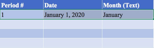
First, we enter the cells for the period, date, and month to start a certain pattern, in this case an entry for January 1, 2020. Then highlight the 3 cells or each of them independently.

And then finally, simply drag down numbers and dates using the bottom right corner button to auto-populate them in sequence to easily populate sequential data. Your final result would look something like this; a clean set of data!

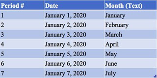
You can also achieve this if you had the data presented horizontally in columns and you had selected a few and dragged them across. As you can see, this a very useful shortcut to save you time if you select a sequence of data and dragged them either up or down. That way, you don’t have to manually type in data into all these cells. That could be especially useful if you are working with a larger data set.

2) How to Count the Days between Dates in Excel

You subtract one value from the other to count the days between two dates. For example, we subtract cell B68 from B69 to find out that there 121 days between the two dates, and similarly 391 days between the cells from B70 and B69.

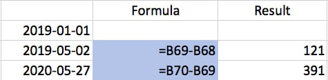
This offers a very quick way to calculate the number of days between dates for purposes such as forecasting!

3) How to Insert Today’s Date in Excel

This formula in Excel is valuable if you want always want a cell to always contain the most current date as the current date. Simply type in a cell, ‘=today()’

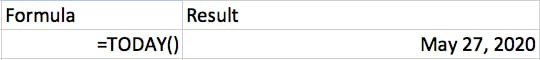
This can be useful as a reference rather than hard-coding a date. As you can see in cell G18, today’s date, as this article was being typed on May 27, 2020.

4) How to Count the Number of Items in a Range in Excel (USING COUNTIF formula)

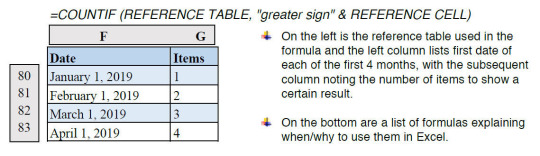
The COUNTIF formula, as the name suggests, helps us count the number of items in a range if it meets certain criteria that you can set manually. The COUNTIF formula can be used with dates as well. Let’s say you want to count the number of dates in a list which are more recent than, let’s say, January 1st, 2019. In that case, we would use the COUNTIF formula to reference the list and use the “greater than (>)” to determine if the dates are greater than the reference date. To Count items in a table if they are more recent than a particular date, enter:

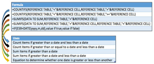
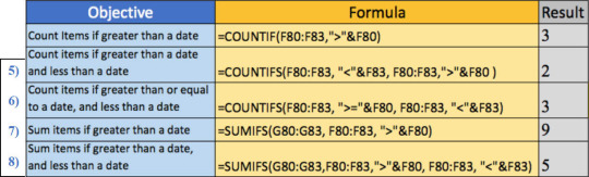
5) How to Count items if greater than a date and less than a date in Excel:

=COUNTIFS(REFERENCE TABLE,”less than”&REFERENCE CELL,REFERENCE TABLE,”greater sign”&REFERENCE CELL)

You should use the COUNTIFS (i.e. plural) formula if you want to set multiple conditions for a lookup and use the date in a table. Use plural when you want to set more than one condition.

6) How to Count items if greater than or equal to a date and less than a date in Excel:

=COUNTIFS(REFERENCE TABLE,”lesser sign”&REFERENCE CELL,REFERENCE TABLE,”greater sign=”&REFERENCE CELL)

Tip 6 is very similar to tip 5. The COUNTIFS formula is used again here but instead of just using the “greater than (>)” or “less than (<)” signs to count the number of dates within a range, we added in an equal (=) sign. If you want to find something greater than or equal to in an Excel formula, just put the two signs beside each other when writing the formula. In cell H26, we are looking for dates greater than or equal to January 1st, 2019, and less than April 1, 2019. So as you can see in the formula, we are using the “greater than (>)” but also, we are putting in the equal sign (=) so that it is greater than or equal to.

7) How to Sum items if greater than a date by in Excel:

=SUMIFS(DATA TO SUM,REFERENCE TABLE,”greater sign”&REFERENCE CELL)

This tip is about integrating the SUMIFS formula with dates. There are three components to the SUMIFS formula. The first part is to reference the data to be summed. The second part is the reference table itself. The third part is the criteria. Let’s say we want to calculate the sum of the items greater than a particular date. For example, on January 1st, 2019 in the table above, we calculate this in cell H27.

8) Sum items if greater than a date and less than a date in Excel

=SUMIFS(DATA TO SUM, REFERENCE TABLE, “greater sign”&REFERENCE CELL, REFERENCE TABLE, “lesser sign”&REFERENCE CELL)

This is similar to Tip 7 but it just shows that we can have multiple conditions in a SUMIF formula. For instance, if we want to calculate the sum of amounts for column E, from rows 80 to 83, we would write it as the formula shown above. First, we select the sum range which in this case is from cells G80-G83, then we select the criteria range which is F80-F83 from the reference table. Lastly, we set up the range with a selection criterion which is our objective of summing items if greater than a date (January 1, 2019) and less than a date (April 1, 2019).

9) How to determine whether one date is greater or less than another in Excel

The following table is an example of using the IF function to count the number of live contracts. The results from the formula are reflected in the table with a “1” if its live, and a “0” if it is inactive. As you can see, we have 1 new contract per month starting with January and ending in April 2018.

The D34 in the formula is the contract date and is set up to be less than E33 which is the month-end date, and return the value 1. That is if the contract is closed before the month’s end, then portray it as 1, i.e. active, otherwise, put 0 for inactive.

The equation to determine whether one date is greater or less than another: =IF(E59 greater than DATE(yyyy,m,dd), value if true, value if false)

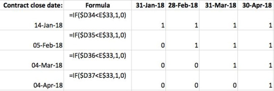
Note also in this formula we put a ‘$’ sign in front of the ‘D’ so that when we drag the formula across, the column does not change with the contract dates. Similarly, we locked the ‘33’ for E33 in the formula so that the row is locked for the date headers being referenced. This application is known as active cell reference and it can be used to lock both the rows and columns when applying ‘$’ sign before both.

10) How to Insert the Month-End date of a referenced cell in Excel

The month-end date formula is a commonly used function in Excel for financial reporting and when creating financial statements. Simply insert the formula of

‘=EOMONTH(reference,0)’ into a cell to quickly formulate the end of month dates.

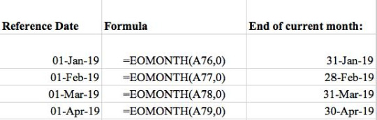
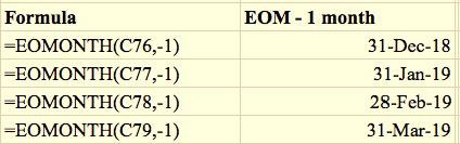
As mentioned before, the reference date was taken from the left column of the reference table.

The ‘End of current month’ for each reference date was found using the EOMONTH formula shown in the middle column.

The zero is used if you want to obtain the end of month date for the current month.

Add 1 for each additional month prior to or after the current month.

For example, the previous month would be -­‐1 and subsequent month would be 1 as shown in the formula section on the left columns.

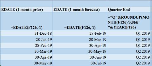
11) How to Insert the quarter-end text of a referenced cell in Excel

To insert the quarter-end text of referenced cell: =”Q”&ROUNDUP(MONTH(REFERENCE CELL)/3,0)&” “&YEAR(REFERENCE CELL)

This is very useful if you work in accounting/finance and often work with large data sets across multiple months, quarters, and years and you often need to summarize the data by quarter.

As shown above, after applying the formula, the result appears with the quarter number followed by the year of the given sample date. The G102 is the first reference cell from the sample date column and it follows with G103, and so forth.

12) How to reference periods for financial modeling in Excel

This is a very effective financial modeling tip that can be used in Excel. Let’s say we are creating a model and you have a list of recurring expenses budgeted in a tab. Some of these are payable monthly, others quarterly, and some are annually and a wise tip is to mark them as the payment frequency. Then, in an assumptions tab, you should have this layout that says payment frequency and the number of payments per period, i.e. 1 for monthly, 3 for quarterly, 12 for annually.

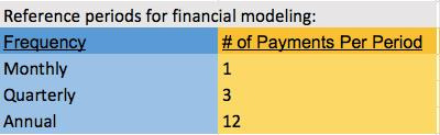
This allows you to then do a lookup against this table in the financial model that you’re working on and return the payments number per period so that you could project out costs for the year. This is just a useful tip on how you want to start thinking about modeling data.

We have translated payment frequency (monthly, annually, and quarterly) into actual numbers and created a table upon which we can later reference in our financial modeling through a VLOOKUP or other type of index so that we can start to apply formula.

Tips 13 through 15 are here to show you how to strip out days, months, and years from a date in Excel.

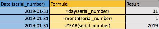
13) How to return the day of a date reference cell in Excel

For instance, let’s say that you just want to return the day of a date cell. In that case, we would just use the day formula shown on the table above. To return the day of a date reference cell, simply enter ‘=day()’ in a cell, and get a result like 31 for this example.

14) How to return the month of a date reference cell in Excel

Similarly, we can use the month formula to strip out the month from the date. In column F, we have an example date that we want to strip the data from and column H we have the data stripped, i.e. 1. To return the month of a date reference cell, simply enter ‘=month()’ in a cell.

15) How to Return the year of a date reference cell in Excel

To return the year of a date reference cell, simply enter ‘=year()’ in a cell.

This is useful if you are working with large pools of data and want to strip out part of it in a column. You can do that with these formulas and then just copy down the formula beside the table that you are working on to strip all of them out at once. You might want to have a column for day, month, year, each of which is stripping data from a reference cell.

Tips 16 through 21 show us how to extract text from a date cell rather than just the number.

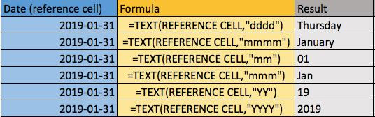
16) How to return the text day of a week of a reference date in Excel

To return the text day of the week of a reference date in Excel, simply type ‘=TEXT(REFERENCE CELL,”dddd”)’ in a cell.

For instance, tip 16 shows that you can extract the day text by using the formula text and then open parenthesis to put in the reference cell and then putting quotations around the letters “dddd”. This would formulate the result as Thursday which is ultimately the day of the week for the date.

17) How to return the text month of a reference date in Excel

To return the text month of a reference date in Excel, simply type ‘=TEXT(REFERENCE CELL, “mmmm”)’ in a cell. This is an important tool in Excel to use when analyzing data from financial statements for a specific month.

18) How to extract the 2-digit month from date cell in Excel

To extract the 2 digit month from date cell in Excel, simply type ‘=TEXT(REFERENCE CELL, “mm”)’ in a cell. If you just want the number of months from a given date in Excel, put 2 m’s, ‘mm’, inside the text formula of a cell.

19) How to extract the 3 letter abbreviation month from date cell in Excel

Another cool feature is using ‘mmm’ which will give you the abbreviated version of the text. For instance, it would write ‘Jan’ for January. To extract the 3 letter abbreviation month from date cell in Excel, simply type ‘=TEXT(REFERENCE CELL, “mmm”)’ in a cell.

20) How to extract the 2-digit year from date cell in Excel

To extract the 2 digit year from date cell, simply type ‘=TEXT(REFERENCE CELL, “YY”)’ in a cell. We can use the ‘yy’ to return the abbreviated version of 2019 to show the last 2 digits, i.e. 19.

21) How to extract the 4-digit year from date cell in Excel

To extract the 4 digit year from date cell in Excel, simply enter ‘=TEXT(REFERENCE CELL, “YYYY”)’ in a cell. We can see here that using 4 Y’s would give us the full year 2019 number on the cell.

22) How to return another date based on the number of months in the future or past in Excel

To return another date based on the number of months in the future or past in Excel, simply type ‘=EDATE(CELL, months)’ in a cell.

This is different from the ‘=EOMONTH’ formula which looked at the month-end date, not the exact date 1 month prior or before like this formula for EDATE is able to achieve.

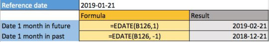
The date format is given by yyyy-mm-dd and it can be changed depending on your preference of formatting.

LASTLY, this table a culmination of all the formulas used in this lesson above and summarizes the most effective date formulas in Excel!

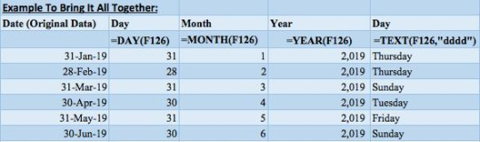
The left side of the table has some reference sample dates. The next column returns the day using the day formula, then the following column returns the month using the month formula, and we have the year to return that as well.

To the right of that, we use the text formula and return the full name of the day, then we use the EDATE formula to return the prior month day, and then the month ahead.

Finally, in the last column, we convert the date to a quarter-end reference using the quarterly reference formula which we reviewed in Tip 11.

These summarize the key date formulas in Excel that you should practice and build it to your daily financial modeling, analysis, or other Excel work. This will ultimately save you time in the analysis that you performed.

Now that we know these formulas are available, when you perform your next tasks on a day to day basis we should ask ourselves before doing the analysis whether any of these formulas are relevant to be used. If the answer is yes, don’t be hesitant to start using them and integrating date formulas into your Microsoft Excel activities!!

I hope that helps. Please leave a comment below with any questions or suggestions. For more in-depth Excel training, checkout our Ultimate Excel Training Course here. Thank you!